Serial Vickrey Mechanism

ISSN (Print) 0473-453X

Discussion Paper No. 1095 ISSN (Online) 2435-0982

The Institute of Social and Economic Research Osaka University

6-1 Mihogaoka, Ibaraki, Osaka 567-0047, Japan

SERIAL VICKREY MECHANISM

Yu Zhou

Shigehiro Serizawa

July 2020

Serial Vickrey mechanism ¹

Yu Zhou ² Shigehiro Serizawa ³ July 30, 2020

Abstract

We study an assignment market where multiple heterogenous objects are sold to unit demand agents who have general preferences accommodat- ing imperfect transferability of utility and income e¤ects. In such a model, there is a minimum price equilibrium. We establish the structural charac- terizations of minimum price equilibria and employ these results to design the “ Serial Vickrey mechanism,” that …nds a minimum price equilibrium in a …nite number of steps. The Serial Vickrey mechanism introduces the objects one by one, and requires agents to report …nite-dimensional prices in …nitely many times. Besides, the Serial Vickrey mechanism also has nice dynamic incentive properties.

Keywords: The assignment market, minimum price equilibrium, general pref- erences, structural characterizations, Serial Vickrey mechanism, dynamic incentive compatibility

JEL Classi…cation: C63, C70, D44

1 The preliminary version of this article is presented at 2017, 2019 Economic Design Con- ferences, SING 13, 2018 SPMID conference, PET 2018, the 14th Meeting of the Society for Social Choice, the 19th SAET, 2019 APIOC, 2019 Nanjing International Conference on Theory of Games and Economic Behavior, and seminars at City University of Hong Kong, ITAM, and Maastricht. We thank Tommy Andersson, Itai Ashlagi, Lawrence Ausubel, Vincent Crawford, Chuangyin Dang, Jean-Jacques Herings, Fuhito Kojima, Scott Duke Kominers, Andy Macken- zie, Debasis Mishra, James Schummer, Ning Sun, Dolf Talman, Alex Teytelboym, Ryan Tierney, William Thomson, and Rakesh Vohra for their helpful comments. We gratefully acknowledge

…nancial support from the Joint Usage/Research Center at ISER, International Joint Research Promotion Program (Osaka University), and Grant-in-aid for Research Activity, Japan Society for the Promotion of Science (15J01287, 15H03328, 15H05728, 19K13653).

2 Graduate School of Economics, Kyoto University, Yoshida-Honmachi, Sakyo-ku, Kyoto, 606- 8501, Japan. E-mail: zhouyu_0105@hotmail.com

3

1 Introduction

In auction and matching theory, quasi-linearity of preferences is commonly as- sumed. ¹ It means that utility can be perfectly transferred among agents or the payment for a good exhibits no income e¤ect for its demand. Quasi-linearity largely simpli…es analysis and makes the duality of linear programming techniques applicable to auction and matching problems (Vohra, 2011). ² Nevertheless, the frictionless world with perfectly transferred utility is rather ideal. Quasi-linearity holds only in restricted environments such as those where payments are negligibly small compared to incomes or there are no budget constraints.

In the spectrum license auctions in OECD countries, regarded as one of the most important applications of the theory, bidders often borrow to pay for the huge bids and face non-linearity of borrowing cost, which makes their preferences non-quasi-linear (Klemperer, 2004). In practical housing markets, income e¤ects and budget constraints also prevail (Zhou and Serizawa, 2018). Distortional taxes in transactions make utility imperfectly transferred (Fleiner et al. 2019).

These practical limitations motivate many researchers to generate new tech- niques to extend the results and gain new insights for auction and matching theory for general preferences that accommodate imperfect transferability of utility and income e¤ects. Such examples include:

Properties of equilibria or stable outcomes in matching models (Crawford and Knoer, 1981; Kelso and Crawford, 1982; Quinzi, 1984; Demange and Gale, 1985; Caplin and Leady, 2014; Alaei et al. 2016; Fleiner et al. 2019; Schlegel, 2020)

E¢ cient, strategy-proof, and fair rules in the assignment market (Sun and Yang, 2003; Andersson and Svensson, 2014, 2018; Morimoto and Serizawa, 2015;

Kazumura et al. 2020a)

Properties of equilibria or stable outcomes in matching models with price controls or hierarchy constraints (Andersson and Svensson, 2014, 2018; Herings, 2018; Kojima et al. 2020)

Mechanism design or optimal auction design without quasi-linearity (Baisa, 2017; Noldeke and Samuelson, 2018; Kazumura et al. 2020b)

The theoretical foundation for empirical research (Galichon et al. 2019) This paper works on one of most prominent models in the matching theory, the assignment market: Multiple heterogenous objects are to be sold to several agents where payments can continuously change, and agents have unit-demand general preferences. We draw on the above …rst two bullet directions, but go

1 See Myerson (1980) and Shapley and Shubik (1972) for example.

2 The recent development of (discrete) convex analysis and tropical geometry techniques relies

on quasi-linearity, e.g., Murota (2003) and Baldwin and Klemperer (2019).

beyond them by studying e¢ cient and dynamic incentive-compatible mechanisms with …nite-dimensional information revelation of agents.

In our settings, when general preferences satis…es standard assumptions of monotonicity and …niteness, there is a minimum price equilibrium (MPE), whose supporting price (vector) is coordinate-wise minimum among all equilibrium prices (Demange and Gale, 1985). The MPE attracts particular attention since the MPE rule, mapping each general preference pro…le to an MPE, is the only rule satisfy- ing e¢ ciency and strategy-proofness, and also has desirable revenue-maximazation property. ³ However, the MPE rules unrealistically require agents to report their whole general preferences, and have neither information of how an MPE is imple- mented, nor any dynamic incentive property.

We design a dynamic mechanism that …nds an MPE, by asking each agent to report a …nite-dimensional price whose coordinate is an “indi¤erence price” in

…nitely many times, instead of requiring each agent to report her full preference.

An agent’s indi¤erence price of an object is her willingness to pay for the object, evaluated from her provisionally assigned bundle (object-payment pair). A quasi- linear preference is presented by an agent’s valuations of the objects, or simply a

…nite-dimensional price. Thus, reporting indi¤erence prices naturally generalizes the information elicitation of quasi-linear preferences to general preferences.

We proceed the mechanism design by providing three structural characteri- zations that show the inner connections between an (arbitrary) equilibrium and an MPE. Proposition 1 establishes the …rst characterization, the “connectedness”

property of the MPE. It says the equivalence of the three conditions: (i) An equi- librium price is an MPE price; (ii) each object is connected via agents’demands;

and (iii) each agent gets either a connected object or nothing.

To show the second and third characterizations, we also show as Lemma 1 that (i) to …nd an MPE from an equilibrium, the object reassignment and price adjustment are within the unconnected objects and agents, i.e., objects and agents without connectedness property, and (ii) the MPE prices of the unconnected ob- jects are bounded below by the indi¤erence prices of the connected agents. Then we build a “I pay others’ indi¤erence prices (IPOIP) process,” to …nd an MPE from an equilibrium. Given a candidate of the MPE assignment, the IPOIP process recursively raises the prices of objects in that assignment from their lower bounds.

Theorem 1 establishes the second characterization: (i) the price and assign- ments of the connected objects in an equilibrium are the same as the MPE, and (ii) the MPE price of the unconnected objects in an equilibrium is the coordinate- wise minimum among the IPOIP prices of all candidate assignments. Theorem 2 establishes the third characterization that if IPOIP process stops raising the prices at some point for a candidate assignment, then the candidate is an MPE

3 See Morimoto and Serizawa (2015), and Kazumura et al. (2020a) for details.

assignment, and the price at that point is the MPE price.

Then, we propose a “Serial Vickrey (SV) mechanism,”by exploring the above structural results. The SV mechanism introduces objects sequentially, and based on an MPE for k objects, it employs the “SV sub-mechanism,” to …nd an MPE for k + 1 objects in a …nite number of steps, established as Theorem 3. When introducing the …rst object, the SV sub-mechansim coincides with the second- price auction mechanism. In general, given an MPE for k objects, the SV sub- mechanism contains two stages. Stage 1 uses the …rst structural result to construct an equilibrium for k + 1 by the “E-generating mechanism,”and identify the agents and objects needed to adjust their assignments and prices in Stage 2, by the

“connected-agent identifying mechanism.” Stage 2 explores the second and third structural results and their by-products to conduct object reassignment and price adjustment by “the MPE-adjustment mechanism.”

Finally, we study the incentive compatibility of the SV mechanism. We observe that the rule induced by the SV mechanism coincides with the MPE rule so it is strategy-proof. We show as Proposition 5 that given an MPE for k objects under the true preferences, revealing the true preferences is a dominant-strategy equilib- rium in the normal game forms induced by both the E-generating mechanism and MPE-adjustment mechanism. We establish as Theorem 4 that given an MPE for k objects under the true preferences, revealing the true preferences is a dominant- strategy equilibrium in the normal game form induced by the SV sub-mechanism for k + 1 objects. Theorem 4 is neither implied by the strategy-proofness of the MPE rule since the number of objects changes, nor by the aggregation of two incentive-compatible mechanisms within an SV sub-mechanism. Besides, we re- mark that in the SV mechanism, agents’ welfare is always increasing with the number of introduced objects.

All our results and the corresponding proof techniques are novel to the existing works for general preferences. We leave the details of this point to the next section.

The remainder is organized as follows: Section 2 discusses the related litera- ture. Section 3 de…nes the model and MPEs. Section 4 graphically illustrates the indi¤erence price and the MPE. Section 5 gives the structural characterizations.

Section 6 presents the SV mechanism. Section 7 analyzes the incentives. Section 8 discusses the SV mechanism as concluding remarks.

2 Related literature

The e¢ cient and incentive-compatible mechanism has been studied in the assign-

ment market for quasi-linear preferences. There are three remarkable results: (i)

The MPE price coincides with Vickrey-Clarkes-Groves (VCG) payment (Leonard,

1983); (ii) Assuming integer valuations of agents, the auction mechanisms of De-

mange et al. (1986), Mishra and Parkes (2010), Andersson and Erlanson (2013), and Liu and Bagh (2019), yield MPEs; (iii) The approximate auction mechanisms of Crawford and Knoer (1981) and Demange et al. (1986) …nd a price that devi- ates from the MPE price within certain boundary. For auctions in (ii) and (iii), the increment n decrement is pre-…xed and agents reveal information of their de- mand sets. However, insights in (i), (ii), and (iii) cannot be extended to general preferences: There is no parallel VCG-type payment for the MPE price. In Ap- pendix D, we exemplify that when conducted in the general preference settings, auctions in (ii) and (iii) either largely overshoot or undershoot the MPE price be- yond boundary estimated in the quasi-linear environments. ⁴ These observations justify the use of indi¤erence prices as the information elicitation for general pref- erences: it is almost impossible to propose a price adjustment process by pre-…xing an increment/decrement and only eliciting the information of agents’demand sets.

For general preferences, the equivalence between equilibria and stable out- comes, and the lattice property of equilibria are widely studied, e.g., Quinzi (1984), Demange and Gale (1985), Fleiner et al. (2019), and Schlegel (2020). These prop- erties are qualitatively di¤erent from our structural results. Exceptions are Caplin and Leahy (2014, 2020) and Alaei et al. (2016), who also study the structural properties of the equilibria.

In the same model as ours, Caplin and Leahy (2014) characterize the MPE price by the graph-allocation structure, which initiates Caplin and Leahy (2020) to employ the homotopy method to study the equilibrium changes in response to parameter changes. Alaei et al. (2016) characterize the MPE price by a recursive system that computes the minimum and maximum price equilibria in all smaller markets with di¤erent numbers of agents and objects. These papers use their struc- tural results to obtain the MPEs. In contrast, the SV mechanism iteratively …nds an MPE, which largely improves computations, and also has appealing dynamic incentive properties. In Section 8, we show the models where the SV mechanism e¢ ciently …nds an MPE, but their results do not, and detail the applications where the SV mechanism …nds certain type of MPEs, but theirs do not.

The existence of equilibria for general preferences is commonly proved by two methods. The …rst one is to operate the Keslo-Crawford type adjustment process to get an approximate equilibrium with the discreteized payments and then take the limit argument, the existence is shown, e.g., Kelso and Crawford (1982), Her- ings (2018), and Kojima et al. (2020). The second one is to establish the existence under the piece-wise linear functions, and show the existence for general utility functions by the point-to-point convergence argument. This method is used by Alkan and Gale (1990) and conveys the proof idea of using the “Scarf Lemma”,

4 In our model, the cumulative o¤er process of Hat…eld and Milgrom (2005) coincides with

the approximate auction mechanism, so it fails to approximate an MPE either.

e.g., Quinzi (1984). The SV mechanism is di¤erent from these methods.

Finally, we discuss how our results di¤er from Andersson and Svensson (2018), Noldeke and Samuelson (2018), and Galichon et al. (2019). In the assignment market with price controls, Andersson and Svensson (2018) construct a …nite ascending-price sequence that …nds an “minimum rationing price equilibrium.”

This sequence terminates at an MPE price in our model. It is not clear how to identify two adjacent prices in the sequence in …nitely many steps so their con- struction is di¤erent from the SV mechanism. Noldeke and Samuelson (2018) study the duality relationship without quasi-linearity in the one-to-one two-sided matching model, and characterize the duality of implementable pro…les and as- signments via the Galois connection. The Galois connection is a pair of mappings, with no information of how to …nd a stable outcome so it is di¤erent from the SV mechanism. Galichon et al. (2019) provide the theoretical model with potential application to structural estimation of imperfectly transferable utilities in the one- to-one two-sided matching model. They de…ne an aggregate equilibrium (AE) that can be characterized by a system of equations in terms of matching pairs. Their proposed AE is di¤erent from the MPE, and the corresponding characterization does not hold for the MPE.

3 The model and minimum price equilibrium

There are a …nite set of agents N and a …nite set of heterogenous objects M where j N j = n and j M j = m. ⁵ Not receiving an object is called receiving object 0. Let L M [ f 0 g .

Each agent has unit demand: She receives at most one object. The bundle for agent i is a pair z _i (x _i ; t _i ) 2 L R , in which agent i receives an object x _i 2 L and pays t _i 2 R . Each agent i has a complete and transitive preference R _i over L R . Let P _i and I _i be the associated strict and indi¤erence relations. Assume the following properties of preferences.

Money monotonicity: For each x _i 2 L, each pair t _i ; t _j 2 R , if t _i < t ⁰ _i , (x _i ; t _i ) P _i (x _i ; t ⁰ _i ).

Finiteness: For each t _i 2 R , each pair x _i ; x _j 2 L, there is t _j 2 R such that (x _i ; t _i ) I _i (x _j ; t _j ).

Money monotonicity states that for a given object, a lower payment makes the agent better o¤. Finiteness says that there is no object that is in…nitely good or bad. A preference R _i is general if it satis…es the above two properties. Let R ^G be the class of general preferences and R (R _i ) _{i 2 N} 2 ( R ^G ) ⁿ be a preference pro…le.

5 Let j j denote the cardinality of a set.

An assignment market is summarized by (N; M; R). We …x N and M through- out the paper, and …x a preference pro…le below until we analyze the incentive issues in Section 7.

An allocation z 2 [L R ] ⁿ is a list of agents’ bundles such that except for object 0, no two agents receive the same object, i.e., z (z _i ) _{i 2 N} = ((x _i ; t _i )) _{i 2 N} such that for each pair i; j 2 N , if x _i 6 = 0 and i 6 = j, then x _i 6 = x _j . We denote the set of allocations by Z.

Let p (p _x ) _{x 2 M} 2 R ^m + be a price (vector). Without loss of generality, assume the price of object 0 and all reserve prices of objects are zero. Agent i ⁰ s demand set at price p is de…ned as D _i (p) f x 2 L : (x; p _x ) R _i (y; p _y ), 8 y 2 L g .

De…nition 1: A pair (z; p) 2 Z R ^m + is an equilibrium if

for each i 2 N , x _i 2 D _i (p) and t _i = p _x

, (E-i) for each y 2 M , if for each i 2 N , x _i 6 = y, then p _y = 0. (E-ii) (E-i) says that each agent i receives a bundle z _i consisting of a demanded object x _i and a payment t _i equal to the price of x _i . (E-ii) says that prices of unassigned objects are zero. Let W and P be the sets of equilibria and equilibrium prices.

Fact 1 (Alkan and Gale, 1990; Demange and Gale, 1985): There is an equilibrium and the set of equilibrium prices is a complete lattice.

Therefore, among all equilibrium prices, there is a unique coordinate-wise mini- mum price p ^min 2 P . A minimum price equilibrium (MPE) is an equilibrium supported by p ^min . Let W ^min W be the set of MPEs. Since indi¤erences in preferences are admitted, MPE allocations may not be unique, but they are welfare-equivalent: for each agent i, each MPE brings her the same welfare, i.e., for each pair (z; p ^min ); (z ⁰ ; p ^min ) 2 W ^min , z _i I _i z ⁰ _i .

4 Illustration of indi¤erence price and MPE

The following graphic tools illustrate the “indi¤erence price” de…ned below, and an MPE. These illustrations also help us understand the concepts and results presented in the next sections.

The indi¤erence price (IP)

By money monotonicity and …niteness, for each z _i 2 L R , each y 2 L, there is a unique payment V _i (y; z _i ) 2 R such that two bundles z _i and (y; V _i (y; z _i )) are welfare-equivalent, i.e., (y; V _i (y; z _i )) I _i z _i . We interpret V _i (y; z _i ) as agent i ⁰ s indi¤erence price (IP) of object y at bundle z _i . The indi¤erence price works as the proxy for agents’preference elicitation.

Suppose that there are two agents i and j , and two objects, A and B . Figure

1 illustrates the indi¤erence prices for two preferences.

Figure 1: Illustration of IPs V _i (B ; z _i ), and V _j (B ; z _j )

Three horizontal lines correspond to objects 0, A, and B. For each point on one of the three lines, the distance between that point and the vertical line denotes the payment, e.g., z _i denotes the bundle consisting of object A and payment t _i . By money monotonicity, moving leftward along the same line makes the agent better o¤, e.g., (0; A) P _i z _i . The agent is indi¤erent between bundles connected by an indi¤erence curve, e.g., for agent i, z _i I _i z _i ⁰ , and for agent j, z _j I _j (B; V _j (B; z _j )).

The IP of object B at z _i is V _i (B ; z _i ) since (B; V _i (B; z _i )) I _i z _i . Similarly, the IP of object B at z j is V j (B; z j ) since (B; V j (B; z j )) I j z j .

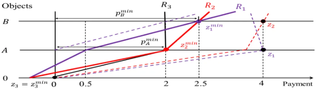
The minimum price equilibrium (MPE) for general preferences

We illustrate an MPE for three agents, 1; 2; and 3, and two objects, A and B, and a preference pro…le where the (real and dotted) lines in purple describe R 1 , lines in red describe R ₂ , and the line in black describes R ₃ .

Figure 2: Illustration of an MPE (z ^min ; p ^min ) for general preferences

We show that (z ^min ; p ^min ) is an MPE. At p ^min = (p ^min _A ; p ^min _B ), D ₁ (p ^min ) = f B g ,

D ₂ (p ^min ) = f A; B g , and D ₃ (p ^min ) = f 0; A g so each agent i receives an object from

her demand set at z ^min and no object is unassigned. Thus (E-i) and (E-ii) holds, and (z ^min ; p ^min ) is an equilibrium.

To see why p ^min is an MPE price, let p ⁰ = (p ⁰ _A ; p ⁰ _B ) be an equilibrium price.

We show p ⁰ p ^min . Since there are three agents and two objects, by (E-i), one agent must demand and be assigned object 0 at p ⁰ . Thus, p ⁰ _A 2 = p ^min _A or p ⁰ _B 2:5 = p ^min _B . In case of p ⁰ _A 2 and p ⁰ _B < 2:5, D ₁ (p ⁰ ) = D ₂ (p ⁰ ) = f B g , contradicting (E-i). In case of p ⁰ _A < 2 and p ⁰ _B 2:5, D 2 (p ⁰ ) = D 3 (p ⁰ ) = f A g , contradicting (E-i). Thus p ⁰ _A p ^min _A and p ⁰ _B p ^min _B .

For quasi-linear preferences, any equilibrium allocation is an MPE allocation, but this statement is not true for general preferences. Let p = (4; 4). It is easy to see that (z; p) is an equilibrium where agent 1 gets A and 2 gets B. However, at p ^min , there is no equilibrium allocation such that 1 gets A and 2 gets B .

5 The structural characterizations

This section establishes structural characterizations of MPEs. The …rst result studies when an equilibrium coincides with an MPE (Proposition 1). The sec- ond and third results disclose a dynamic relation between an equilibrium and an MPE (Theorems 1 and 2). These characterizations are fundamental to design the mechanism that …nds an MPE in Section 6.

5.1 Characterization by connectedness

First, we introduce two concepts: “connected object” and “connected agent.”

De…nition 2: An object x 2 M is connected at (z; p) 2 Z R ^m + if (i) x is unassigned or (ii) there is a sequence f i g =1 of distinct agents ( > 1) that forms a demand connectedness path (DCP) such that

(ii-1) x _i

= 0 or p _x

1

= 0, (ii-2) x _i = x,

(ii-3) for each 2 f 2; ; g , x _i 6 = 0 and p _x

> 0, and (ii-4) for each 2 f 1; ; 1 g , f x _i ; x _i

g 2 D _i (p).

De…nition 2 says that an object x is connected in two cases. In Case (i), object x is unassigned. In Case (ii), there is a sequence of distinct agents such that the …rst agent receives an object with zero price (ii-1); the last agent receives object x (ii-2); each agent who is not the …rst agent gets an object with a positive price (ii-3); each agent who is not the last agent demands his assigned object and the object assigned to her successive agent (ii-4). These agents form a demand connected path to object x. Example 1 illustrates.

Example 1 (Figure 2): At (z ^min ; p ^min ), object B is connected by a DCP formed

by agents 1, 2, and 3 where = 3, i ₁ = 3, i ₂ = 2, and i ₃ = i = 1: (i) x ^min ₃ = 0,

(ii) x ^min ₁ = B, (iii) x ^min ₂ = A, p ^min _A = 2, and x ^min ₁ = B, p ^min _B = 2:5, and (iv) f 0; A g 2 D ₃ (p ^min ) and f A; B g 2 D ₂ (p ^min ). (i) to (iv) corresponds to (ii-1) to (ii-4) in De…nition 2.

De…nition 3: An agent i 2 N is connected at (z; p) 2 Z R ^m + if x _i is connected or x i = 0.

De…nition 3 says that an agent is connected if she gets either a connected object or object 0. Let N C and M C be the sets of connected agents and objects. Let N _U N n N _C and M _U M n M _C be the sets of unconnected agents and objects.

Example 2 illustrates.

Example 2 (Figure 2): At the MPE (z ^min ; p ^min ), N = N _C = f 1; 2; 3 g and M = M _C = f A; B g . Let p = (4; 4). At the equilibrium (z; p), N _C = f 3 g , N _U = f 1; 2 g , and M = M _U = f A; B g .

We give a further remark of connected objects and agents.

Remark 1: (i) Since unassigned objects are connected, the existence of connected objects does not imply the existence of connected agents.

(ii) The connectedness of objects is not applicable to object 0. Thus the existence of connected agents does not imply the existence of connected objects.

(iii) By De…nition 2(ii-1), an agent who gets an object with zero price is connected.

(iv) A connected agent exists () Some agent gets an object with zero price. ⁶ Proposition 1 characterizes the MPE by connected agents and objects.

Proposition 1: Let (z; p) be an equilibrium, and N _C and M _C be de…ned at (z; p).

Then, the following are equivalent:

(i) p = p ^min , (ii) N = N _C , and (iii) M = M _C .

The proof of Proposition 1 is relegated to Appendix A.1. Proposition 1 gives three equivalent conditions to judge whether an equilibrium is an MPE, i.e., (i) the equilibrium price is an MPE price, or (ii) all the agents are connected, or (iii) all the objects are connected. Example 2 also illustrates Proposition 1.

5.2 Characterizations by I-pay-others’-indi¤erence-prices process

In this section, we relate an MPE to an arbitrary equilibrium via a dynamic process. First, we introduce the notation of “the ranking of indi¤erence prices of some object.” Consider an object x, an allocation z and a group N ⁰ of agents.

6 “ ( ” comes from Remark 1(iii). For “ ) ”, by contradiction, suppose that for each i 2 N ,

p x

> 0. Since N C 6 = ; , for each i 2 N C , p x

> 0. Thus for an arbitrary connected agent i,

there is a sequence f i g =1 of distinct agents satisfying De…nition 2, with x i

= 0 or p x

= 0,

contradicting that for each i 2 N , p x

> 0.

We ask each agent i 2 N ⁰ to report her IP V _i (x; z _i ) of x at z _i . Let C ^h (x; z _N

) be the h-th highest IP of x from z among N ⁰ agents. Let C ₊ ^h (x; z _N

) max f C ^h (x; z N

); 0 g . If N ⁰ = N , we write z instead of z N . In case of N ⁰ = ; , let C ₊ ^h (x; z _N

) = 0. Example 3 illustrates.

Example 3 (Figure 2): Let N ⁰ = f 1; 3 g , x = A, and z = z ^min . Since V 3 (A; z ₃ ^min ) = 2 > 0:5 = V ₁ (A; z ₁ ^min ) > 0, then C ₊ ² (A; z ^min _{f 1;3 g} ) = C ² (A; z _f ^min _{1;3 g} ) = V ₁ (A; z ₁ ^min ) = 0:5.

Lemma 1 shows what properties of an equilibrium can preserve at an MPE.

Lemma 1: Let (z; p) be an equilibrium and N _U and M _U be de…ned at (z; p). Let (z ^min ; p ^min ) be an MPE. Then,

(i) j N _U j = j M _U j ,

(ii) for each x 2 M _U , C ₊ ¹ (x; z _N

) p ^min _x < p _x , and (iii) for each i 2 N _U , x ^min _i 2 M _U .

The proof of Lemma 1 is relegated to Appendix A.2. Lemma 1(i) and 1(iii) say that to obtain an MPE from an equilibrium, we only need to reallocate un- connected objects among unconnected agents. Lemma 1(ii) says that for each unconnected object x, its MPE price is upper bounded by its equilibrium price p _x and lower bounded by the maximum value C ₊ ¹ (x; z _N

) of reported indi¤erence prices of object x by connected agents at their equilibrium allocation z _N

. Lemma 1(i) is con…rmed by M U and N U at the equilibrium (z; p) in Example 2. Lemma 1(ii) and (iii) are con…rmed by comparing (z ^min ; p ^min ) and (z; p) in Example 2.

Second, we de…ne the “I-pay-others’-indi¤erence-prices process.” Let be an assignment or bijection, from M _U to N _U , and _i be the associated object assigned to agent i 2 N U . Let be the set of all such assignments.

De…nition 4: Let (z; p) be an equilibrium and N _U and M _U be de…ned at (z; p).

Let 2 . The k I pay-others’-indi¤erence-prices (IPOIP) process for is de…ned as follows: For each x 2 M _U and each i 2 N _U ,

(i) p ⁰ _x C ₊ ¹ (x; z _N

) and z ⁰ _i ( _i ; p ⁰

i

), and (ii) for each s = 1; k,

p ^s _x C ¹ (x; z ^s _N ¹

U

) and z ^s _i ( _i ; p ^s

i

):

The k IPOIP process for a given assignment contains k rounds. It updates the prices and agents’ bundles recursively: First, set the starting price of each unconnected object x as p ⁰ _x = C ₊ ¹ (x; z _N

). Each unconnected agent i is assigned an unconnected object _i and gets the bundle z ⁰ _i = ( _i ; p ⁰

i

). Each unconnected agent i reports her IP of each unconnected object x at z ⁰ _i , i.e., V _i (x; z ⁰ _i ). Then the price of x is updated to the maximum value of all reported IPs, i.e., p ¹ _x = C ₊ ¹ (x; z ⁰ _N

U

).

Each unconnected agent i keeps the same object _i but pays an updated price p ¹

i

, i.e., z ¹ _i = ( _i ; p ¹

i

). In the same manner, the price of each unconnected object x is updated to p ² _x = C ₊ ¹ (x; z ¹ _N

U

) and so forth. The formation of agent’s tentative

payment p ^s _x is in the spirit of the VCG payment. Example 4 illustrates a one-round IPOIP process.

Example 4 (Figure 2): In Example 2, recall N _C = f 3 g , N _U = f 1; 2 g , and M _U = f A; B g at the equilibrium (z; p). Consider an assignment such that agent 1 gets B and 2 gets A. In this case p ⁰ _A = C ₊ ¹ (A; z N

) = C ₊ ¹ (A; z 3 ) = 2, p ⁰ _B = C ₊ ¹ (B; z ₃ ) = 2, z ⁰ ₁ = (B; 2) and z ⁰ ₂ = (A; 2). Then p ¹ _A = C ₊ ¹ (x; z ⁰ _{f 1;2 g} ) = max f V ₁ (A; z ⁰ ₁ ); V ₂ (A; z ⁰ ₂ ) g = 2 and p ¹ _B = max f V ₁ (B; z ⁰ ₁ ); V ₂ (B; z ⁰ ₁ ) g = 2:5.

Let p ^s ( ) be the price generated in round s in a k IPOIP process for . It is easy to see that prices in the process are non-decreasing. Formally, we have:

Fact 2: Let (z; p) be an equilibrium and N _U and M _U be de…ned at (z; p). Let 2 . In the k IPOIP process for , for each s = 1; ; k, we have p ⁰ ( ) p ¹ ( ) p ^s ( ).

Now we give the characterizations of MPEs in terms of IPOIP processes.

Theorem 1: Let (z; p) be an equilibrium, and N _C , M _C , N _U , and M _U be de…ned at (z; p). Let p ^min be the MPE price. Then the following holds.

(i) For each x 2 M _C , p ^min _x = p _x , and for each i 2 N _C , z _i is an MPE bundle.

(ii) There is 2 such that

(ii-1) is an MPE assignment among unconnected agents, and (ii-2) for each x 2 M _U , p ^min _x = p ^j _x ^M

^{j 1} ( ) = min

0

2 p ^j _x ^M

^{j 1} ( ⁰ ).

The proof of Theorem 1 is relegated to Appendix A.3. The proof sketch is as follows. First, we show Theorem 1(i). We argue that if the prices of connected objects decrease, these objects will be “overdemanded” at the MPE price. Thus, their MPE price should be the same as the given equilibrium prices. Then by Lemma 1(ii), connected agents could keep the same equilibrium bundles as their MPE bundles.

Second, we show Theorem 1(ii). For (ii-1), by Fact 1 and Theorem 1(i), there must exist an MPE assignment that assign the unconnected objects to the uncon- nected agents. For (ii-2), it contains two Steps.

Step 1 shows that if is an MPE assignment, then at each round of the IPOIP process, at least one unconnected object’s price reaches its MPE price, and it never increases in the later round. Since there are j M _U j unconnected objects, starting from round 0, the IPOIP process for …nds the MPE price for unconnected objects at most by j M _U j 1 rounds. Thus, for each unconnected object x, p ^min _x = p ^j _x ^M

^{j 1} ( ). Step 2 shows that for any non-MPE assignment ⁰ , at each round of the IPOIP process, at least one unconnected object’s price exceeds its MPE price and by Fact 2, it never decreases in the later round. Since there are j M _U j unconnected objects, for each unconnected object x, p ^min _x p ^j _x ^M

^{j 1} ( ⁰ ).

If all the objects are connected at the given equilibrium, then Theorem 1

coincides with Proposition 1. The novelty of Theorem 1 deals with the case where

there are unconnected agents at the given equilibrium.

Remark 2: Given ⁰ 2 , p ^{j M}

^{j 1} ( ⁰ ) is generally not an equilibrium price for unconnected objects. Thus, Theorem 1(ii-2) is di¤erent from the meet operation of equilibrium prices that generates a new equilibrium price, by their lattice property.

Intuitively, if is an MPE assignment and p ^s obtained at some round s in the k IPOIP process for is an MPE price, then in the later rounds, the price remains unchanged, i.e., p ^s = = p ^k . Theorem 2 surprisingly shows that for any assignment , if the prices in two adjacent rounds s 1 and s of the IPOIP process for remain unchanged, i.e., p ^{s 1} = p ^s , then p ^{s 1} is an MPE price and is an MPE assignment of unconnected objects and agents.

Theorem 2: Let (z; p) be an equilibrium, and N _U and M _U be de…ned at (z; p).

Let p ^min be an MPE price. Let 2 . In the j M _U j IPOIP process for , the following are equivalent:

(i) There is some s j M _U j such that p ^{s 1} = p ^s ;

(ii) is an MPE assignment and p ^{s 1} is the MPE price of unconnected agents and objects.

The proof of Theorem 2 is relegated to Appendix A.4. The proof sketch is as follows. First we show (ii) ) (i). As argued in Step 1 of the proof Theorem 1(ii-2), when p ^{s 1} is the MPE price of unconnected objects and is an MPE assignment of unconnected agents, p ^{s 1} remain unchanged in the later round of the IPOIP process so p ^{s 1} = p ^s .

Next, we show (i) ) (ii). Since the outcome of the IPOIP process may not assign unconnected agents bundles in their demand sets, we de…ne weak connected objects and agents by relaxing (ii-4) in De…nition 2: Agents on the path are indi¤erent between their bundles and the successive agents’ bundles. The proof contains …ve steps. Step 1 shows that all the unconnected objects are weakly connected at ( ; p ^{s 1} ). Steps 2 and 3 show that the price of unconnected objects generated by the IPOIP process is bounded above by their MPE price. Step 4 shows that each unconnected agent i weakly prefer ( _i ; p ^{s 1}

i

) to the bundles consisting of connected objects paired with their MPE price. Step 5 concludes that (ii) holds.

In Example 4, for the assignment where agent 1 gets B and 2 gets A, it is easy to see p ¹ = p ² . By Theorem 2, p ¹ = p ^min and is an MPE assignment.

6 Serial Vickrey mechanisms

6.1 Sketch of Serial Vickrey mechanisms

Based on the obtained structural characterizations in Section 5, we design a

“Serial Vickrey (SV) mechanism,” that …nds an MPE in a …nite number

of steps. The SV mechanism introduces objects one by one and sequentially em- ploys “SV sub-mechanism,”to …nd an MPE for k +1 objects, based on an MPE for k objects.

De…nition 5: The SV mechanism is de…ned as follows. Each agent is initially assigned (0; 0). Introduce object sequentially by its index, 1; 2; .

Step k( 1) introduces object k, and run the SV sub-mechanism for k objects, which is described in De…nition 6. If k = m, stop at the output of the SV sub- mechansim. Otherwise, go to Step k + 1.

Remark 3: By Fact 1, the MPE price for the assignment market (N; M; R) is unique so how we index the objects in M does not matter in the SV mechanism.

The central part of the SV mechanism is the SV sub-mechanism. When the

…rst object is introduced, it coincides with the second-price auction mechanism.

Now we de…ne the SV sub-mechanism for k + 1 objects where 0 k < m.

De…nition 6: Let (z ^min ; p ^min ) be an MPE for k objects. The SV sub-mechanism for k + 1 objects is de…ned as follows.

Stage 1: Operate the “E-generating mechanism,” (De…nition 8, Section 6.2), to generate an equilibrium (z; p) for k + 1 objects from (z ^min ; p ^min ). Then run the “N C -identifying mechanism,” (De…nition 9, Section 6.2), to identify the set of connected agents N C at (z; p). If all agents are connected, i.e., N C = N , then terminate at (z; p). Otherwise, identify M _U and N _U , and go to Stage 2.

Stage 2: Operate the “MPE-adjustment mechanism,”(De…nition 11, Sec- tion 6.3), to identify the MPE allocation of unconnected agents N _U .

In the SV sub-mechanism, agents report …nite-dimensional prices composed of indi¤erence prices in …nitely many times. We will establish:

Theorem 3: Given an MPE for k objects, the SV sub-mechanism …nds an MPE for k + 1 objects via agents’reports of …nite-dimensional prices in …nitely many times.

We prove Theorem 3 via Propositions 2 and 3 in Section 6.2, and Proposition 4 in Section 6.3, which shows the properties of the E-generating mechanism, N _C - identifying mechanism, and the MPE-adjustment mechanism, respectively. As a direct outcome, we have:

Corollary 1: The SV mechanism …nds an MPE in a …nite number of steps via agents’reports of …nite-dimensional prices in …nitely many times.

6.2 Stage 1 of SV sub-mechanism

We …rst introduce a process to identify the demand connected path for a given

object, which is key to establish the E-generating mechanism.

De…nition 7: Demand-connectedness-path-…nding (DCP-…nding) process for object x Let x 2 M be a connected object that is assigned to agent i, i.e., x i = x, at (z; p) 2 Z R ^m + .

Phase 1: Round 1: Set N ₁ f i g . If p _x = 0, stop the process.

If p _x > 0, set N ₂ f j 2 N n N ₁ : x 2 D _j (p) g and go to Round 2.

Round s( 2): Set L s f y 2 L : x j = y for some j 2 N s g .

If there is y 2 L _s s.t. y = 0 or p _y = 0, stop Phase 1 and go to Phase 2.

Otherwise, set N _s+1 f j 2 N n [ ^s k=1 N _k : D _j (p) \ L _s 6 = ;g and go to Round s + 1. ⁷ Phase 2: Let S be the …nal round of the process. Then, construct a sequence f i _s g ^S s=1 of distinct agents as follows: (i) Choose i ₁ 2 N _S such that x _i

= 0 or p _x

1

= 0, and (ii) for each j 2 f 2; ; S g , choose i j 2 N S+1 j such that x i

2 L S+1 j and x _i

2 D _i

(p).

The DCP-…nding process works as follows: pick a connected object x that is assigned agent i. In Phase 1, if the price of x is zero, we are done and it contains a trivial DCP. If not, i.e., p _x > 0, we collect the demanders N ₂ of x by excluding agent i. Since x is connected and p _x > 0, N ₂ 6 = ; . If there is some agent in N ₂ , say, agent j, who obtains an object x _j with zero price, then agent j is connected to x by her demand, i.e., f x; x _j g 2 D _j (p) and we are done. Otherwise, we collect the set L ₂ of objects assigned to agents in N ₂ , and repeat the process till some agent obtains an object with zero price. In Phase 2, we trace back from the agent who gets an object with zero price to object x via the DCP. Example 5 illustrates.

Example 5 (Figure 2): Consider a DCP-…nding process for object B at (z ^min ; p ^min ).

Recall that agent 1 gets B, i.e., i = 1 and x ₁ = B .

In Phase 1, at Round 1, we set N ₁ = f 1 g . Since p ^min _B > 0, we need to …nd all the agents who demand B , except for agent 1. It is just the agent 2 so N ₂ = f 2 g . Then we come to Round 2 and collect agent 2 ⁰ s assigned object, i.e., L ₂ = f A g . Since p ^min _A > 0, we need to …nd all the agents who demand A, except for agents 1 and 2. It is just the agent 3 so N ₃ = f 3 g . Since x ^min ₃ = 0. We stop Phase 1 and go to Phase 2.

In this case S = 3. Phase 2 constructs a DCP consisting of a sequence of agents f 3; 2; 1 g , i.e., i ₁ = 3, i ₂ = 2, and i ₃ (= i _S ) = 1.

The following result summarizes the property of DCP-…nding process.

Lemma 2: Let (z; p) 2 Z R ^m + . Let x 2 M be an assigned connected object.

(i) Phase 1 of DCP-…nding process stops in a …nite number of rounds.

(ii) The sequence f i _s g ^S s=1 of distinct agents of Phase 2 is a DCP for object x.

By the …niteness of N , Lemma 2(i) holds. By construction, the sequence f i _s g ^S s=1 in Lemma 2(ii) satis…es (ii-1) to (ii-4) in De…nition 2. The demand sets

7 In such a case, since for each y 2 L _s , y is connected and p _y > 0, N _s+1 6 = ; .

used to identify the DCPs can be derived from the agents’reported indi¤erence prices at the given allocation.

Now we are ready to propose the E-generating mechanism.

De…nition 8: E-generating mechanism Let (z ^min ; p ^min ) be an MPE of k objects. Introduce a new object y, i.e., the object indexed by number k + 1.

Phase 1: Each agent i reports V _i (y; z _i ^min ), and compute C ¹ (y; z ^min ).

If C ¹ (R; y; z ^min ) 0, set (z; p) as

(a) p _y = 0, and p = (p ^min ; p _y ), and (b) for each i 2 N , z _i = z _i ^min . Otherwise, go to Phase 2.

Phase 2: Arbitrarily select an agent i with the highest IP of y at z _i ^min , i.e., V _i (y; z _i ^min ) = C ¹ (y; z ^min ). Run the DCP-…nding process for x ^min _i at (z ^min ; p ^min ), and obtain a DCP f i g =1 for x ^min _i . Set (z; p) as

(a) p _y = C ₊ ² (y; z ^min ), and p = (p ^min ; p _y ), (b) z _i = (y; p _y ),

(c) for each i _l 2 f i g 1 ¹ , z _i

= z _i ^min

, and (d) for each j 2 N nf i g 1 , z _j = z ^min _j .

The essence of E-generating mechanism is Phase 2. It works as follows. When object y is introduced, each agent reports her IP of y at z _i ^min , i.e., V _i (y; z _i ^min ).

We assign the new object to an arbitrary agent i whose has the highest IP, but ask her to pay the second highest IP (in the spirit of the second-price auction).

We identify a DCP for agent i ⁰ s assignment x ^min _i at (z ^min ; p ^min ). After agent i is assigned object y, we alternate the bundles of agents on the identi…ed DCP from the object with zero price. All other agents remain their bundles at z ^min . Such an construction generates an equilibrium for k + 1 objects. Example 6 illustrates.

Example 6 (Figures 2 and 3): Given (z ^min ; p ^min ) in Figure 2, we introduce object C and illustrate the E-generating mechanism by Figure 3.

Figure 3: Illustration of an E-generating mechanism

In Phase 1, each agent i reports her IP for C at z _i ^min : V ₁ (C; z ₁ ^min ) = 3, V ₂ (C; z ₂ ^min ) = 2:5, and V ₃ (C; (0; 0)) = 1. Since C ¹ (C; z ^min ) = V ₁ (C; z ₁ ^min ) > 0, go to Phase 2.

In Phase 2, we set p _C = C ₊ ² (C; z ^min ) = 2:5 and p = (p ^min _A ; p ^min _B ; p _C ). We assign object C to agent 1, but ask her to pay C ₊ ² (C; z ^min ). Thus, agent 1 is assigned (C; 2:5). Recall Example 2 for the DCP of object B, which consists of agents 3, 2, and 1. We alternate the bundles of agents 3 and 2 along this path:

z ₃ = z ₂ ^min = (A; 2) and z ₂ = z ₁ ^min = (B; 2:5).

In Example 6, the constructed (z; p) is an equilibrium. Formally, we can show:.

Proposition 2 (Property of E-generating mechanism): Let (z ^min ; p ^min ) be an MPE for k objects. Introduce object y. Then the E-generating mechanism

…nds an equilibrium (z; p) for k + 1 objects in a …nite number of phases.

The proof of Proposition 2 is relegated to Appendix B.1. The following mech- anism identi…es the set of connected agents N _C at some given equilibrium.

De…nition 9: N _C -identifying mechanism Let (z; p) be an equilibrium.

Round 1: Let N ₁ f i 2 N : p _x

= 0 g . If N ₁ = ; , set N = ; and stop the process.

Otherwise, go to Round 2.

Round s( 2): Let

M ^{s 1} f y 2 M nf x _i : i 2 [ ^s k=1 ¹ N _k g : p _y > 0, y 2 D _i (p) nf x _i g for some i 2 N _{s 1} g . If M ^{s 1} = ; , set N = [ ^s k=1 ¹ N _k and stop the process.

Otherwise, let N _s f i 2 N : x _i = y for some y 2 M ^{t 1} g , and go to Round s + 1.

In words, N _C -identifying mechanism works as follows: at the equilibirum (z; p), we collect a set N ₁ of the agents who get objects with zero prices. Then we collect a set M ¹ of objects in the demand sets of agents in N ₁ , except for their assigned objects. Since objects in M ¹ have positive prices, they must be assigned to some agents. Then we identify the set N ₂ of agents who are assigned objects from M ¹ , and repeat the process. The collection of the identi…ed agents in N ₁ , N ₂ ,:::, are connected agents. Formally, we get the result below.

Proposition 3 (Property of N _C -identifying mechanism): Let (z; p) be an equilibrium. Then the N _C -identifying mechanism stops in a …nite number of rounds and N is the set of connected agents at (z; p).

The proof of Proposition 3 is relegated to Appendix B.2. To con…rm Proposi- tion 3, in Figure 2, at (z; p), agent 3 is the only connected agent so N ₁ = N = f 3 g . Once N _C is identi…ed, M _C , N _U , and M _U can be immediately obtained.

6.3 Stage 2 of SV sub-mechanism

Theorems 1 and 2 imply that by conducting a IPOIP process for each assignment

in , we can …nd an MPE from an equilibrium. However, it is possible to …nd

an MPE (i) without conducting IPOIP processes for all assignments in , and (ii) while reducing the number of rounds during a IPOIP process. Such ideas are embodied into Stage 2 of SV sub-mechanism.

Theorem 1 and Lemma 1(ii) imply that some assignments can be disquali…ed as the MPE assignments before and after conducting the IPOIP process. They reduce the number of assignments needed to be operated via the IPOIP processes.

As direct outcomes of Theorem 1 and Lemma 1(ii), we have:

Fact 3 (Disquali…cation before and after IPOIP process): Let (z; p) be an equilibrium. Let agent i and object x be unconnected at (z; p).

(i) If V _i (x; z _i ) C ₊ ¹ (x; z _N

) = p ⁰ _x , then no MPE assignment gives x to i.

(ii) Let 2 and z ^{j M}

^{j 1} ( ) be the outcome of the ( j M _U j 1) IPOIP process for . If V _i (x; z ^j _i ^M

^{j 1} ( )) < C ₊ ¹ (x; z _N

) = p ⁰ _x , no MPE assignment gives x to i.

The implication of Fact 3 is as follows. Given an equilibrium generated by Stage 1 of SV sub-mechanism, if it is not an MPE, we use Fact 3(i) to examine assignments in . Let DQ 0 be the set of initial disquali…ed assignments. ⁸ We remove DQ ₀ from and ⁰ = n DQ ₀ be the initial candidate set.

After operating the IPOIP process for some , we obtain its outcome z ^{j M}

^{j 1} ( ).

Using Fact 3(ii), we examine assignments in again. Let DQ( ) be the set of disquali…ed assignments after the IPOIP process for . ⁹ We remove DQ( ) from . Whenever we conduct IPOIP process for some , we remove DQ( ) from the current candidate set of MPE assignments.

Example 7 illustrates Fact 3 by introducing agent 4 to Figure 3 in Example 6.

Example 7 (Figure 3): Suppose that V ₄ (A; (0; 0)) = V ₄ (B; (0; 0)) = 1, and V ₄ (C; (0; 0)) = 2. Let z ₁ ⁰ = z ₁ = (C; 2:5), z ₂ ⁰ = z ₂ = (B; 2:5), z ₃ ⁰ = z ₃ = (A; 2), z ₄ ⁰ = (0; 0), and p ⁰ = p where z and p are depicted in Example 6. It is easy to see that (z ⁰ ; p ⁰ ) is an equilibrium for the assignment market with agents f 1; 2; 3; 4 g and objects f A; B; C g . At (z ⁰ ; p ⁰ ), N _U ⁰ = f 1; 2; 3 g , N _C ⁰ = f 4 g , M _U ⁰ = M.

In this case, = f (A; B; C); (A; C; B); (B; A; C); (B; C; A); (C; A; B); (C; B; A) g . For each x 2 M _U ⁰ , C ₊ ¹ (x; z _N ⁰

C

) = V 4 (x; z ₄ ⁰ ).

By V ₁ (A; z ₁ ⁰ ) < C ₊ ¹ (A; z _N ⁰

C

), V ₁ (B; z ₁ ⁰ ) = C ₊ ¹ (B ; z _N ⁰

C

), and Fact 3(i), agent 1 never gets A or B at any MPE so DQ ₀ = f 2 : ₁ = A; B g . We remove DQ ₀ from .

Let = (C; A; B) and assume p ^{j M}

^{j 1} ( ) = (2; 2; 2). Then, z ^j ₃ ^M

^{j 1} ( ) = (B; 2). By V ₃ (C; z ^j ₃ ^M

^{j 1} ( )) = 1 < 2 = C ₊ ¹ (A; z _N ⁰

C

) and Fact 3(ii), agent 3 never gets C at any MPE. Since (B; A; C) 2 DQ ₀ is removed, DQ( ) = f (A; B; C) g is further removed from a candidate set after the IPOIP process for .

8 DQ 0 f 2 : 9 i 2 N U ; V i ( _i ; z) < p ⁰

g where p ⁰

= C ₊ ¹ (x; z N

).

9 DQ( ) f ⁰ 2 : 9 i 2 N U ; 9 x 2 M U s.t. ⁰ _i = x and V i (x; z ^j _i ^M

^{j 1} ( )) < p ⁰ _x g where

p ⁰ _x = C ₊ ¹ (x; z N

)

Before showing how to reduce the number of rounds during a IPOIP process, we introduce the following concept.

De…nition 10: Let 2 and p ⁰ 2 R ^{j M}

^j . Assignment survives in the k IPOIP process against p ⁰ if p ^k ( ) p ⁰ and for some x 2 M _U , p ^k _x ( ) = p ⁰ _x .

In other words, an assignment does not survive in the k IPOIP process against p ⁰ if there is some x 2 M _U whose price p ^k ( ) exceeds p ⁰ _x or the price p ^k ( ) is detached from the initial price p ⁰ coordinate-wisely. By Lemma 1(ii) and Theorems 1 and 2, we have:

Fact 4 (Disquali…cation during IPOIP process): If an assignment 2 does not survive in the j M _U j IPOIP process against any equilibrium price p, then

is not an MPE assignment.

Putting Facts 3 and 4 together, we present the following mechanism.

De…nition 11: MPE-adjustment mechanism Let (z; p) be an equilibrium, and N _U and M _U be de…ned at (z; p).

Session 0: Identify . Each unconnected agent i reports V _i (x; z _i ) of each uncon- nected object x. Set ⁰ n DQ ₀ , ⁰ (x _i ) _{i 2 N}

, and p ⁰ (p

) _{x 2 M}

. Then, go to Session 1.

Session s( 1): Choose _s 2 ^s and conduct the j M _U j IPOIP process for _s . Set ^{1 0} , p ¹ = p ⁰ , ¹ = ⁰ , and choose ₁ = ⁰ . Then, one of following three cases occurs:

Case 1 : If p ^r ( _s ) = p ^{r 1} ( _s ) at round r j M U j , then stop the process at (z ; p ) such that _s and p p ^r ( _s ).

Case 2: If Case 1 fails to hold, but _s survives the j M _U j IPOIP process against p ^s , then set ^s+1 _s and p ^s+1 p ^{j M}

^{j 1} ( _s ). Collect the disquali…ed set DQ( _s ), and set ^{s+1 s} n (DQ( _s ) [ f s g ). Then, go to Session s + 1.

Case 3: If both Case 1 and Case 2 fail to hold, set ^{s+1 s} , p ^s+1 p ^s , and ^{s+1 s} nf s g . Then, go to Session s + 1.

The MPE-adjustment mechanism works as follows. Given an equilibrium (z; p), we identify the unconnected agents N _U and objects M _U . In Session 0, each uncon- nected agent i reports her IP V _i (x; z _i ) at z _i to each unconnected object x. Using Fact 3(i), we obtain the initially candidate set of assignments ⁰ . Then we set the equilibrium assignment and price at (z; p) as the initial reference assignment and price, i.e., ⁰ (x _i ) _{i 2 N}

and p ⁰ (p

) _{x 2 M}

.

In Session 1, set ^{1 0} , ¹ = ⁰ , and p ¹ = p ⁰ . We choose ₁ = ⁰ and run the j M U j IPOIP process for ₁ . We meet one of three cases. In Case 1, if at round r j M _U j , the price remain the same as round r 1, i.e., p ^r ( ₁ ) = p ^{r 1} ( ₁ ), by Theorem 2, ₁ and p ^r ( ₁ ) are the MPE for unconnected agents and objects.

Case 2 deals with the situation where Case 1 fails to hold, but ₁ survives against

p ¹ . Then we update the reference assignment and price by ² ₁ and p ²

p ^{j M}

^{j 1} ( ₁ ). Using Fact 3(ii), we collect the disquali…ed assignments DQ( ₁ ) for

1 and remove DQ( ₁ ) and ₁ from ¹ . Set ^{2 1} n (DQ( ₁ ) [ f 1 g ) and proceed to Session 2. If neither Case 1 nor Case 2 holds, using Fact 4, we keep the reference assignment and price unchanged. We just remove ₁ from ¹ and set

2 1

nf 1 g . Then we proceed Session 2, and repeat above process. Formally, we have the following result.

Proposition 4 (Property of MPE-adjustment mechanism): Let (z; p) be an equilibrium. The MPE-adjustment mechanism generates a sequence f ( ^t ; p ^t g ^T t=0

such that

(i) T < + 1 , and for each t = 1; ; T , p ^t p ^{t 1} .

(ii) ^T and p ^T are MPE assignment and price of unconnected agents and objects at (z; p).

The proof of Proposition 4 is relegated to Appendix B.3. Propositions 2, 3, and 4 together establish Theorem 3. Notably, if the assignment of a given equilibrium (z; p) is just an MPE assignment, then the MPE-adjustment mechanism stops at Session 1. This happens for certain classes of preferences detailed in Section 8.

7 Incentive compatibilities

In this section, we investigate the incentive properties of the SV mechanism. A rule f is a mapping from the set of general preference pro…les ( R ^G ) ⁿ to the set of allocations Z. It assigns each agent i with a bundle f i (R) at each preference pro…le R. A rule f is strategy-proof if no agent can gain from misreporting her preference, i.e., for each R 2 ( R ^G ) ⁿ , each i 2 N , and each R ⁰ _i 2 R ^G , f _i (R _i ; R _i ) R _i f _i (R ⁰ _i ; R _i ).

In our model, the MPE rule that assigns each general preference pro…le an MPE is strategy-proof (Demange and Gale, 1985; Morimoto and Serizawa, 2015).

Let f ^SV be the rule that selects the outcome of the SV mechanism. By Theorem 3, f ^SV coincides with the MPE rule.

Fact 5: The rule f ^SV is strategy-proof on the set of general preference pro…les.

Fact 5 says that in the normal game form induced by f ^SV where agents’ac- tions are revealing their preferences, truthfully revealing is a dominant-strategy equilibrium.

The SV mechanism is decomposed into m steps, i.e., m SV sub-mechanisms.

Each SV sub-mechanism is decomposed into two stages, i.e., the E-generating

and MPE-adjustment mechanisms. We show that these sub-mechanisms are also

incentive compatible. In other words, even if agents are not fully rational and

their perspectives are limited to the step or the stage where they are interact-

ing, agents have incentives to reveal true preferences. Stage-wise and step-wise

incentive compatibilities are remarkable properties of the SV mechanism.

We …rst study the cases in which agents’ perspectives are limited to stages, and analyze the incentive properties of the E-generating and MPE-adjustment mechanisms. Note that the outcomes of these mechanisms depend both on the revealed preferences and allocations obtained from previous steps or stages. Thus, we need to introduce some notations.

For each k 2 N ⁺ , let Z ^k f z 2 Z : 8 i 2 N; x _i 2 f 0; 1; : : : ; k gg be the set of allocations for k objects (together with object 0). If k = m, then Z ^k = Z.

Given k; k ⁰ 2 N ⁺ , an augmented rule from k to k ⁰ , g ^{k ! k}

: ( R ^G ) ⁿ Z ^k ! Z ^k

, associates each preference pro…le R and an allocation z with k objects, to an allocation g ^{k ! k}

(R; z) with k ⁰ objects. Let g _i ^{k ! k}

( ; ) be the bundle assigned to agent i. Given an allocation z 2 Z ^k , g ^{k ! k}

( ; z) induces a normal game form. If all agents’actions are revealing their preferences, (g ^{k ! k}

; R) forms a revelation game.

De…nition 12: Let k; k ⁰ 2 N ⁺ , R 2 ( R ^G ) ⁿ , and z 2 Z ^k . Revealing R is a (weakly) dominant-strategy from z in g ^{k ! k}

( ; z) if for each i 2 N , each R ⁰ _i 2 R ^G , and each R _i 2 ( R ^G ) ^{n 1} , g _i ^{k ! k}

(R _i ; R _i ; z) R _i g _i ^{k ! k}

(R ⁰ _i ; R _i ; z).

Consider the case of k = 0 and k ⁰ = j M j . Then Z ⁰ = f 0 g where 0 (0; 0) _{i 2 N} . Let g ^{0 !j M j} ( ; 0) = f ^SV ( ). Then revealing R is a dominant-strategy equilibrium from 0 in g ^{0 !j M j} ( ; 0) if and only if f ^SV ( ) is strategy-proof.

Let g ^sub1 ( ; ) be the augmented rule from k to k + 1 such that if z 2 Z ^k is an MPE allocation for R, g ^sub1 (R; z) selects the outcome of the E-generating mechanism in the SV sub-mechanism for k + 1 objects. Notice that g ^sub1 ( ; z) depends on both the preferences revealed in the E-generating mechanism and recorded DCPs at z 2 Z ^k , which depends on the preferences revealed in Step k of the SV mechanism.

Let g ^sub2 ( ; ) be the augmented rule from k + 1 to k + 1 such that if z 2 Z ^k+1 is an equilibrium allocation for R, g ^sub2 (R; z) selects the outcome of the MPE-adjustment mechanism in the SV sub-mechanism for k + 1 objects. Notice that g ^sub2 ( ; z) depends both on the preferences revealed in the MPE-adjustment mechanism and the recorded N _C , N _U , M _C and M _U at z 2 Z ^k+1 , which depends on the preferences revealed in Stage 1 in the SV sub-mechanism for k + 1 objects Proposition 5: Let 0 k < j M j and R 2 ( R ^G ) ⁿ .

(i) For each z 2 Z ^k , if z is an MPE allocation for R, then revealing R is a dominant-strategy equilibrium from z in g ^sub1 ( ; z).

(ii) For each z 2 Z ^k+1 , if z is an equilibrium allocation for R, then revealing R is a dominant-strategy equilibrium from z in g ^sub2 ( ; z).

The proof of Proposition 5 is relegated to Appendix C.1. Proposition 5 states

“stage-wise strategy-proofness” of the SV sub-mechanism. In Stage 1, when a

new object is introduced, no agent can gain by misreporting. In Stage 2, at the

equilibrium obtained in stage 1, no agent can gain by misreporting. Thus, even if

agents’perspectives are myopic and limited to the stages where they are currently interacting, agents have incentives to reveal their true preferences.

Finally, we investigate the cases in which agents’perspectives are beyond stages but limited to steps, and show that the SV sub-mechanism, the composition of above two mechanisms, is also incentive compatible. Let g ^sub ( ; ) be the aug- mented rule from k to k + 1 such that if z 2 Z ^k is an MPE allocation for R, g ^sub (R; z) coincides with the outcome of the SV sub-mechanism for k + 1 objects.

Notice that g ^sub ( ; z) depends on both the preferences revealed in the SV sub- mechanism for k + 1 objects, and the recorded information on DCPs at z 2 Z ^k which depends on the preferences revealed in Step k in the SV mechanism.

Theorem 4: Let 0 k < j M j and R 2 ( R ^G ) ⁿ . For each z 2 Z ^k , if z is an MPE allocation for R, then revealing R is a dominant-strategy equilibrium from z in g ^sub ( ; z).

The proof of Theorem 4 is relegated to Appendix C.2. Theorem 4 states “step- wise strategy-proofness” of the SV sub-mechanism. Theorem 4 is not implied by Fact 5, since at each step, the SV sub-mechanism involves a di¤erent number of objects. As discussed below, it is not implied Proposition 5 either.

To see how Theorem 4 works, we discuss its sketch proof idea. We …x an agent i and show that she cannot bene…t from misreporting. We …rst give some facts and then construct three lemmas, as the preliminary results. Fact C.1 extends Fact 5 by introducing reserve price. Fact C.5 shows that given an MPE, the MPE allocation of any subset of agents that includes all unconnected agents, is an MPE with reserve price of the subeconomy that excludes the remaining agents and sets the reserve price of each object as the maximum value of all reported IPs by those excluded agents at the given MPE. Facts C.2 to C.4, Fact C.6, and three lemmas show how prices are adjusted and objects are reallocated, and identify the set of agents and objects that preserve the connectedness or unconnectedness properties at the outcome of Stage 1, when agent i misreports.

We complete the proof by considering two cases. In Case I, agent i is connected (at the outcome of Stage 1) under truthful reporting. We show that agent i is always connected even if she misreports. By Proposition 5(i), this implies that agent i never gains by misreporting in Stage 1. Thus, by Theorem 1(i), she cannot gain from misreporting.

In Case II, agent i is unconnected under truthful reporting. By misreporting, agent i can indirectly in‡uence the outcome of Stage 2 by making the set of unconnected agents unchanged, expanded or shrunk at the outcomes of Stage 1.

Such impacts invalidate Proposition 5(ii). We develop new techniques that employ Fact C.5 so that Fact C.1 implies that agent i cannot gain from misreporting.

We end this section by discussing the welfare property of the SV mechanism.

First, agents’welfare is non-decreasing with the number of introduced objects in