Chapter 4 Scattering of X-ray from a crystal

Graduate School of Engineering, Nagoya Institute of Technology

“Crystal Structure Analysis”

Takashi Ida (Advanced Ceramics Research Center) Updated Nov. 05, 2013

!

Chapter 4 Scattering of X-ray from a crystal

Now we are going to treat the diffraction from a crystal. In Chaps. 4 and 5, it will be shown that the diffraction condition will naturally be derived, simply by calculating the structure factor (Fourier transform of electron density distribution) of a crystal.

Do NOT assume that “a crystal is periodical arrangement of atoms”, because we can never ignore the effect of thermal vibration of atoms, when we measure the diffraction intensity at room temperature. As the atoms in a crystal are thermally vibrating at a finite temperature, the snap shot of the atomic position should look like that “atomic positions are randomly deviated from

periodically arranged average position”. Strictly speaking, the atoms are not periodically located at a realistic crystal.

Furthermore, the typical frequency of the atomic vibration should be in the range of microwave or infrared wave, that is, , then the atoms will appear almost stationary at random positions, when you look at the atoms by X-ray with more rapid frequency of . It is known that the amplitude of the thermal vibration of atoms at room temperature should be about 0.1 Å = 0.01 nm. Since this amount is comparable to the broadness of the electron density considered in Chap. 3, it is concluded that “we cannot neglect the effect of thermal vibration”.

!

4-1 Thermal vibration

First, let us examine the amplitude of the thermal vibration of the atoms in a realistic materials at room temperature.

The simplest way to treat the thermal vibration of atoms in a solid body is the assumption of

“harmonic oscillator” having a natural frequency. The thermal vibration of atoms should be three- dimensional, but it can be reduced to the combination of one-dimensional vibrations, when the motion along three directions are independent of each other.

One-dimensional harmonic oscillator is a fundamental mechanical model. You should have learned the eigen-energy and eigen-states of a hormonic oscillator in lectures about quantum mechanics, but in this section, the harmonic oscillator is treated in terms of classical mechanics.

Let the amplitude be , and force constant k, then the energy of vibration will be given by (Hooke’s law). The displacement at the time t should be expressed by , and the mean squared value of the displacement is given by

, (4.1)

!

10¹⁰ ~ 10¹⁴ s⁻¹

10¹⁸~ 10²⁰ s⁻¹

x_max 1

2k x_max² x=x_maxe^2πiνt

Δx

( )

Δx ^{2= Re}

( )

^{x 2 = 1}

1 /ν x_max² cos²(2πνt)dt

0 1/ν

∫

= x_max² 1 /ν

1+cos(4πνt)

2 dt

0

1/ν

∫

^{=νxmax2 ⎡}_⎣⎢2^{t +sin(4πνt}_8πν ^)⎤_⎦⎥

0 1/ν

= x_max² 2

and the root of the mean squared value of the displacement is given by

. (4.2)

The probability that the state of energy E is realized at the temperature T should be given by the Maxwell-Boltzman distribution function,

!

( kB : Boltzman constant ),

and substitution: will give the normal (Gaussian) distribution of the amplitude, , the broadness of which is given by the standard deviation .

The force constant k should depend on the strength of the interatomic bonds, but we can roughly evaluate it from the elastic properties of a solid body. You will find the values of the volume compressibility of most of solid materials lie in . As the linear

compressibility should approximately be 1/3 of the volume compressibility for isotropic materials, it should be about . When we assume the representative value of the linear compressibility to be , and the interatomic distance to be 0.2 nm, the force constant is estimated at

.

Then the amplitude of the thermal vibration at room temperature (300 K) should be

.

So we may conclude that the amplitude of the thermal vibration is about 0.01 nm = 0.1 Å at room temperature. The amplitude of the thermal vibration is independent of the weight of atom, while the frequency should be affected by the weight. Actually, a simple assumption: “all the atoms are vibrating with the amplitude of 0.1 Å” works well in many cases.

The model assuming independent oscillators is called “Einstein model for thermal vibration”.

In contrast, “Debye model” can treat collective motion of atoms, and can incorporate the correlation of the atomic displacement, in principle. Roughly speaking, the correlation of the atomic displacement should be taken into account only at lower temperatures than about 100 K, and the Einstein model will not look too much simplified at room temperature. The traditional way of crystal structure analysis assumes the Einstein model about the thermal vibration of the atoms.

! !

!

4-2 Effects of thermal vibration and scattering from crystals

As the oscillation of the electric field of the X-ray is much more rapid than the natural thermal vibration of the atoms, the atoms will appear stationary when you look at them by X-ray, and the

Δx= x_max 2

f_MB(E)=e^−E/kBT

1.3806503(24)×10⁻²³ [J K⁻¹] E= 1

2k x_max² exp −k x_max²

2k_BT

⎛

⎝⎜

⎞

⎠⎟ k_BT /k

0.5 ~ 3×10⁻¹¹ Pa^-1

0.1 ~ 1×10⁻¹¹ Pa^-1 0.3×10⁻¹¹ Pa^-1

k=

(

1 [Pa]

) (

^{0.2×10−9[m]}

)

²

0.3×10⁻¹¹

( )

^×

(

^{0.2×10−9[m]}

)

^{≈0.7×102 [N m−1]}

k_BT

k =

(

1.38×10⁻²³[J K⁻¹]

)

^×

(

^{300 [K]}

)

0.7×10² [N m⁻¹]

⎡

⎣⎢

⎢

⎤

⎦⎥

⎥

1/2

≈8×10⁻¹²[m]=0.008 [nm]

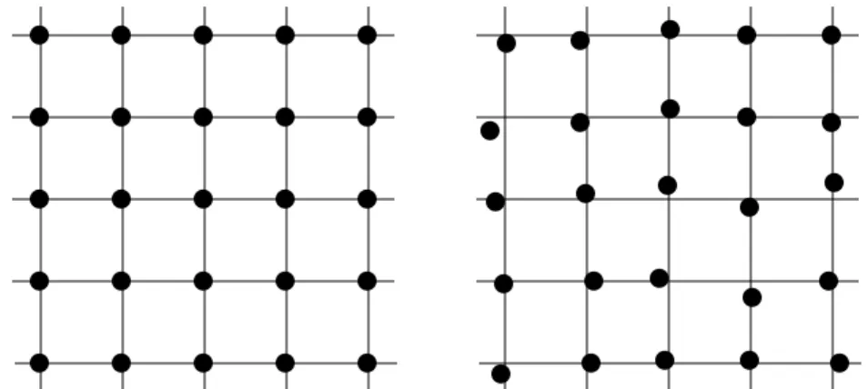
atoms will appear displaced from periodically located average positions, as schematically illustrated in Fig. 4.1.

!

    

Fig. 4.1 Schematic illustration of atomic positions at 0 K (left) and room temperature (right).

The atomic position should look randomly located around the average position.

!

What scattering is expected from such a realistic crystal ?

We can still assume that the “average” atomic positions are periodically arranged in a crystal.

The units of three dimensional periodicity of averaged positions are represented by three vectors, , and . When the average position of the j-th atom among M atoms in the unit structure is represented by , the average positions of all the atoms in the crystal can be expressed by

( , , : integer ). By adding the atomic displacement

caused by thermal vibration, the atomic position of an arbitrary atom will be given by

!

. (4.3)

!

The total electron density of the crystal should be the sum of each electron density of an atom

located at the position , that is,

. (4.4)

It should be noted that the electron density of a collection of atoms cannot be exactly equal to the sum of the electron density of each atom, because the electron density should be modified by chemical bonds in a solid body, and what keeps the solid state is nothing but the chemical bonds.

But the proportion of the change caused by chemical bonds is not large in the total electron density, particularly in inorganic materials or metals, where the number of inner-shell electrons is much larger than that of the valence electrons. The modification of the electron density caused by

chemical bonds is sometimes discussed in terms of difference between the calculated intensities and experimental intensities based on a highly precise diffraction measurement, but the start point should still be the model based on the sum of the scattering from isolated atoms.

a! !

b c!

r!_j r!_ξηζj =ξa!+η!

b+ςc!+ r!_j ξ η ζ Δr!_ξηζj

r!_ξηζj= r!_ξηζj +Δr!_ξηζj =ξa!+η!

b+ςc!+ r!_j +Δr!_ξηζj

ρ_j(r!−r!_ξηζj) r!_ξηζj ρ_total(r!)= ρ_j

(

r!−r!_ξηζj

)

j=1

∑

M ξ

∑

,η,ζ

= ρ_j r!−ξa!−η!

b−ςc!− r!_j − Δr!_ξηζj

( )

j=1

∑

M ξ

∑

,η,ζ

As the structure factor to express the scattering intensity from whole the crystal is the Fourier transform of the total electron density, it should be expressed by

.

Here a simplified expression is used instead of . Transformation of the equation for the structure factor follows,

,

.

(4.5) Note that the factor:

(4.6)

in Eq. (4.5) is nothing but the atomic scattering factor introduced in Chap. 3. By utilizing the atomic scattering factor for the j-th atom , the structure factor of a crystal should be given by

.

(4.7) Next, let us consider the average structure factor, when the statistical distributions of atomic positions are known. Assume that the probability distribution density function of the displacement of the j-th atom is given by a function , and that all the atoms ( atoms for N unit cells) vibrate independently (with no correlation). Then the average structure factor should be given by

!

,

(4.8)

F_total(!

K)= ρtotal(! r)

R

∫

^{3 exp 2πi}

(

^K!⋅r!

)

^dv

= exp 2πi! K⋅!

(

r

)

R

∫

^{3 ρj}

(

^{!r−ξa!−ηb!−ςc!− !rj − Δr!ξηζj}

)

j=1

∑

M

ξ,η,ζ

∑

^dv

!

R

∫

^{3 dv !dxdydz}

−∞

∞

∫

−∞

∞

∫

−∞

∞

∫

=↑

!dx

∫∑ ⁼∑∫^!dx

exp 2πi "

K⋅"

(

r

)

R

∫

^{3 ρj}

(

^{r"−ξa"−ηb"−ςc"− r"j − Δr"ξηζj}

)

j=1

∑

M

ξ

∑

,η,ζ ^dv

=↑

!r≡r!′+ξa+η! !

b+ςc+! r!_j +Δr!_ξηζj

exp 2πi !

K⋅ r!′+ξ! a+η!

b+ς! c+ !

r_j +Δ! r_ξηζj

( )

⎡⎣ ⎤

R

∫

³ ⎦^ρj

^{( )}

^r!′

j=1

∑

M

ξ,η,ζ

∑

^dv′

=↑ f(x)g(y)dx

∫

! g(y)∫f(x)dx

exp 2πi "

K⋅ ξ"

a+η"

b+ς"

(

c

)

⎡⎣ ⎤⎦

ξ

∑

,η,ζ ^{exp 2π⎡}⎣ ^iK"⋅

(

^{r"j +Δr"ξηζj}

)

⎤

j=1 ⎦

∑

M ^ρj

^{( )}

^{r"′ exp 2π}

(

^iK"⋅r"′

)

R

∫

^{3 dv′}

ρj(r!′)

R

∫

^{3 exp 2π}

(

^iK!⋅r!′

)

^{dv′= fj}

( )

^K!

f_j(! K) F_total(!

K)= exp 2πi ! K⋅ ξ!

a+η! b+ς!

(

c

)

⎡⎣ ⎤⎦

ξ

∑

,η,ζ ^{fj(K!)exp 2π}

(

^{iK!⋅ r!j}

)

^{exp 2π}

(

^{iK!⋅ Δr!ξηζj}

)

j=1

∑

M

Δ!

r_j g_j Δ!

r_j

( )

^N×M

F_total(!

K) = "

R

∫

^{3 "}

R

∫

^{3 "}

R

∫

^{3 Ftotal(K!)}

R

∫

³

×g₁(Δ! r_ξ

1η₁ζ₁1)"gM(Δ! r_ξ

1η₁ζ₁M)"g1(Δ! r_ξ

Nη_Nζ_N1)"gM(Δ! r_ξ

Nη_Nζ_NM)

×d(Δv_ξ

1η₁ζ₁1)"d(Δv_ξ

1η₁ζ₁M)"d(Δv_ξ

Nη_Nζ_N1)"d(Δv_ξ

Nη_Nζ_NM)

!

which is a -fold multiple integral. It may look quite complicated, but the assumption of the independence of atomic displacements greatly simplifies the formula, because most of the integrals will disappear by applying the following relation,

!

  . (4.9)

!

In conclusion, we can derive the following formula for the average structure factor, on the assumption of independence :

      . (4.10)

When we define a function:

, (4.11)

the average structure factor of a crystal is given by

. (4.12)

The function defined by Eq. (4.11), , represents the “Laue’s condition” to determine the condition that diffraction occurs, similarly to the “Bragg’s condition” treated in Chap. 1, and it can also represent the effect of finite size of a crystallite, as will be shown in Chap. 6. The meaning of the function will be described in Chaps. 5 & 6 in more detail.

When we define the last integral part in Eq. (4.12) as a function :

, (4.13)

Eq. (4.12) is further simplified as

(4.14)

The function defined by Eq. (4.13) is called the “atomic displacement factor”. It was previously called “temperature factor” or “Debye-Waller factor”, but the term “atomic

displacement factor” is currently recommended by the International Union of Crystallography.

Dynamical displacement by thermal vibration and static displacement by other origins (impurity, structural defects, for example) cannot be distinguished by a usual X-ray diffraction measurement.

Now, we have already obtained almost the complete formula for the average structure factor of a crystal in Eq. (4.14), where the effect of thermal vibration of atoms are taken into

account. But, ... is it enough to describe the realistic measurement of X-ray diffraction ? The diffraction intensity data obtained by a realistic measurement may correspond to the squared

absolute value of the structure factor, , where is the complex

conjugate of . N×M

exp 2πi ! K⋅ Δ!

r_ξηζj

( )

^{gj′(Δr!ξ ′′η ′ζ ′j)}

R

∫

^{3 d(Δvξ ′′η ′ζ ′j)=exp 2π}

(

^{iK!⋅ Δr!ξηζj}

)

^{gj′(Δr!ξ ′′η ′ζ ′j)d(Δvξ ′′η ′ζ ′j)}

R

∫

³

=exp 2πi ! K⋅ Δ!

r_ξηζj

( ) [

^{ξ ≠ ′ξ} or η ≠ ′η or ς ≠ ′ς or j≠ ′j

]

F_total(!

K) = exp 2πi ! K⋅ ξ!

a+η! b+ς!

(

c

)

⎡⎣ ⎤⎦

ξ

∑

,η,ζ ^{fj(K!)exp 2π}

(

^{iK!⋅ r!j}

)

j=1

∑

M

× g_j(Δ!

r)exp 2πi ! K⋅ Δ!

(

r

)

^d(Δv

R

∫

^{3 )}

G(!

K)≡ exp 2πi ! K⋅ ξ!

a+η! b+ς!

(

c

)

⎡⎣ ⎤⎦

ξ,η,ζ

∑

F_total(!

K) =G(!

K) f_j(!

K)exp 2πi ! K⋅ !

r_j

( )

j=1

∑

M ^{gj(Δr!)exp 2π}

(

^{iK!⋅ Δr!}

)

^d(Δv

R

∫

^{3 )}

G(! K)

G(! K) T_j(!

K)≡ g_j(Δ!

r)exp 2πi ! K⋅ Δ!

(

r

)

^d(Δv)

R

∫

³

F_total(!

K) =G(!

K) f_j(! K)T_j(!

K)exp 2πi ! K⋅ !

r_j

( )

j=1

∑

M

T_j(! K)

F_total(! K)

F_total(!

K)² =F_total^* (!

K)F_total(!

K) F_total^* (!

K) F_total(!

K)

Finally, let us examine what is the difference between the averaged value of squared absolute value of the structure factor and the squared absolute value of the average structure

factor .

From Eq. (4.7), we obtain

, (4.15)

and

.

(4.16) Then the average of the squared absolute value of the crystal structure factor should be

!

,

(4.17) and the value of each integral in Eq. (4.17) should be

, (4.18)

only when and and and , and

. (4.19)

Then, we will have

,

F_total(! K)² F_total(!

K) ²

F_total^* (!

K)= exp −2πi ! K⋅ ′ξ !

a+η′! b+ς′!

(

c

)

⎡⎣ ⎤⎦

ξ′

∑

,η′,ζ′

× f_j^*_′(!

K)exp −2πi ! K⋅ !

r_j′

( )

^exp

⁽

^{−2πiK!⋅ Δr!ξ ′′η ′ζ ′j}

⁾

′ j=1

∑

M

F_total(!

K)²= exp 2πi !

K⋅ (ξ − ′ξ )!

a+(η − ′η)!

b+(ς − ′ς )!

(

c

)

⎡⎣ ⎤⎦

ξ′

∑

,η′,ζ′ ξ

∑

,η,ζ

× f_j(! K)f_j^*_′(!

K)exp 2πi ! K⋅ !

r_j − ! r_j′

( )

( )

⎡⎣ ⎤

⎦exp 2πi ! K⋅ Δ!

r_ξηζj− Δ! r_{ξ ′′η ′ζ ′j}

( )

⎡⎣ ⎤⎦

′ j=1

∑

M j=1

∑

M

F_total(!

K)² = "

R

∫

^{3 "}

R

∫

^{3 "}

R

∫

^{3 Ftotal(K!)2}

R

∫

³

×g1(Δ! r_ξ

1η1ζ11)"g_M(Δ! r_ξ

1η1ζ1M)"g₁(Δ! r_ξ

NηNζN1)"g_M(Δ! r_ξ

NηNζNM)

×d(Δv_ξ1η1ζ11)!d(Δv_ξ1η1ζ1M)!d(Δv_ξNηNζN1)!d(Δv_ξNηNζNM)

= exp 2πi !

K⋅ (ξ − ′ξ )!

a+(η − ′η )!

b+(ς − ′ς )!

(

c

)

⎡⎣ ⎤⎦

ξ′

∑

,η′,ζ′

ξ

∑

,η,ζ ^{fj(K!)fj*′(K!)}

′ j=1

∑

M j=1

∑

M

×exp 2πi ! K⋅ !

r_j − ! r_j′

( )

⎡⎣ ⎤

⎦ "

R

∫

^{3 "}

R

∫

^{3 "}

R

∫

^{3 exp 2π}_⎡⎣ ^{iK!⋅ Δ}

(

^{r!ξηζj− Δr!ξ ′′η ′ζ ′j}

)

_⎤⎦

R

∫

³

×g₁(Δ! r_ξ

1η₁ζ₁1)"gM(Δ! r_ξ

1η₁ζ₁M)"g1(Δ! r_ξ

Nη_Nζ_N1)"gM(Δ! r_ξ

Nη_Nζ_NM)

×d(Δv_ξ

1η₁ζ₁1)!d(Δv_ξ

1η₁ζ₁M)!d(Δv_ξ

Nη_Nζ_N1)!d(Δv_ξ

Nη_Nζ_NM)

g_j

R

∫

^{3 (Δrξηςj)d(Δvξηςj)=1}

ξ =ξ′ η=η′ ς =ς′ j= j′ exp 2πi !

K⋅ Δ!

r_ξηζj− Δ! r_{ξ ′′η ′ζ ′j}

( )

⎡⎣ ⎤⎦

R

∫

³

R

∫

^{3 gj(Δr!ξηζj)gj′(Δr!ξ ′′η ′ζ ′j)d(Δvξηζj)d(Δvξ ′′η ′ζ ′j)}

=T_j(! K)T_j^*_′(!

K)

F_total(! K)² =

j=1

∑

M

ξ

∑

,η,ζ ^{fj (K!)2}

+

ξ,η,ζ

∑

j=1

∑

M ^{exp 2π}⎡⎣ ^iK!⋅

(

^{(ξ − ′ξ )a!+(η − ′η )b!+(ς − ′ς )c!}

)

⎤⎦

(ξ′,η′,ζ′,

∑

j′)≠(ξ,η,ζ,j)

×f_j(! K)f_j^*_′(!

K)exp 2πi ! K⋅ !

r_j − ! r_j′

( )

⎡⎣ ⎤

⎦T_j(! K)T_j^*_′(!

K)

, (4.20)

and find the following relation,

. (4.21)

Therefore, the value of the averaged squared absolute value of structure factor may be slightly different from the squared absolute value of the averaged structure factor . However, has a value with the order of -times multiplication of a unit cell structure factor, while the deviation has a value with the order of -times multiplication of a unit cell structure factor. So we may neglect the difference between them, unless the crystallite is very small.

!

4-3 Atomic displacement factor

The atomic displacement factor introduced in Eq. (4.13) can be defined not only for the harmonic oscillator but for any kind of statistical distribution about atomic displacement. What we should assume in the formulation of Eq. (4.13) is independence of the vibration (displacement) of each atoms.

!

4-3-1 Isotropic atomic displacement factor

The effects of atomic displacement is simple, when we can assume isotropic thermal vibration and three-dimensional Gaussian (normal) distribution of displacement. Such statistical distribution of displacement is just “three-dimensional harmonic oscillator” discussed in Sec. 4-1. The

distribution of atomic displacement is given by

(4.22)

where is the mean squared displacement of the j-th atom. We have already solved the Fourier transform of this type of distribution in Sec. 3-2-1. The solution of the atomic displacement factor is

. (4.23)

When we define

, (4.24)

the atomic displacement factor can be expressed by

. (4.25)

=N

j=1

∑

M ^fj(K!)2

(

^1−Tj(K!)2

)

^{+ G(K!)2}

^∑

_j=1^{M fj(K!)Tj(K!)exp 2π}

⁽

^{iK!⋅ r!j}

⁾

²

F_total(!

K)² = F_total(!

K) ²+N f_j(! K)²

j=1

∑

M

(

^1−Tj(K!)2

)

F_total(! K)² F_total(!

K) ² F_total(!

K) ² N²

N

g_j(!

r)= 1

(2π)^3/2U_j^3/2exp − r² 2U_j

⎛

⎝⎜

⎞

⎠⎟

U_j

T_j(!

K)≡ g_j(!

r)exp 2πi ! K⋅!

(

r

)

^dv

R

∫

³

=exp

(

−2π²K²U_j

)

^=exp⎛_⎝⎜^−8π2U_λ^{jsin2 2Θ⎞}_⎠⎟

B_j =8π²U_j

T_j(K)=exp −B_jsin²Θ λ²

⎛

⎝⎜

⎞

⎠⎟

Traditionally, the parameter Bj defined by Eq. (4.24) was used for treating the effect of thermal vibration, and called “atomic displacement parameter” or “temperature parameter”. Certainly, the use of Bj instead of Uj makes the calculation a little economized, and typical value of Bj around

“1 Ų” looks more convenient than the value of Uj around “0.01 Ų”. It is sometimes

recommended to use Uj as “mean squared atomic displacement parameter” rather than Bj , and it is easy to get the value of Uj from Bj, anyway . Just divide Bj by .

!

4-3-2 Anisotropic atomic displacement

When the vibration (or statistical displacement) of an atom is not isotropic, the mean squared displacement is varied on direction, and is specified by a matrix

(4.26)

with elements defined by

, , ,

, , . (4.27)

The mean squared deviation along an arbitrary direction is given by , where is the normalized (unit) vector along the direction. Since the length of the projection of displacement

onto the direction is given by , the mean squared value is given by

!

(4.28)

!

When the eigenvalues or principal values of the matrix are given by U1, U2, U3 and the associated eigenvectors or principal axes are given by

, , , (4.29)

8π² =78.9568

U_j=

U_jxx U_jxy U_jzx U_jxy U_jyy U_jyz U_jzx U_jyz U_jzz

⎛

⎝

⎜⎜

⎜⎜

⎞

⎠

⎟⎟

⎟⎟

(Δx)²g_j

R

∫

^{3 (r!)dv≡Ujxx (Δy)2gj}

R

∫

^{3 (r!)dv≡Ujyy (Δz)2gj}

R

∫

^{3 (r!)dv≡Ujzz}

(ΔxΔy)g_j

R

∫

^{3 (r!)dv≡Ujxy (ΔyΔz)gj}

R

∫

^{3 (!r)dv≡Ujyz (ΔzΔx)gj}

R

∫

^{3 (r!)dv≡Ujzx}

u!^t U_j !

u ! u

Δ! r =

Δx Δy Δz

⎛

⎝

⎜⎜

⎜

⎞

⎠

⎟⎟

⎟

u!= u_x u_y u_z

⎛

⎝

⎜⎜

⎜

⎞

⎠

⎟⎟

⎟ Δ!

r⋅! u

Δ! r⋅!

u² = ! u^tΔ!

( )

r

( )

^{Δr!tu! =u!t Δr!Δr!t u!}

= ! u^t

Δx Δy Δz

⎛

⎝

⎜⎜

⎜

⎞

⎠

⎟⎟

⎟

(

Δx Δy Δz

)

^{u! =u!t ΔxΔxΔxΔy ΔxΔyΔyΔy ΔzΔxΔyΔz}

ΔzΔx ΔyΔz ΔzΔz

⎛

⎝

⎜⎜

⎜

⎞

⎠

⎟⎟

⎟ u!

= ! u^t

U_xx U_xy U_zx U_xy U_yy U_yz U_zx U_yz U_zz

⎛

⎝

⎜⎜

⎜⎜

⎞

⎠

⎟⎟

⎟⎟

u!

= ! u^t U !

u

p!₁= p_1x p_1y p_1z

⎛

⎝

⎜⎜

⎜⎜

⎞

⎠

⎟⎟

⎟⎟

p!₂= p_2x p_2y p_2z

⎛

⎝

⎜⎜

⎜⎜

⎞

⎠

⎟⎟

⎟⎟

p!₃= p_3x p_3y p_3z

⎛

⎝

⎜⎜

⎜⎜

⎞

⎠

⎟⎟

⎟⎟

the following relation :

,

is satisfied, that is,

!

, (4.30) and then

, (4.31)

and similarly, the relations :

(4.32)

(4.33)

will also be satisfied. The above three equations Eq. (4.31)-(4.33) are summarized as

.

(4.34) When we define a matrix :

, (4.35)

a relation for the diagonalization :

(4.36)

is derived.

Here the matrix is an orthogonal matrix, and the transposed matrix of an orthogonal matrix is equal to the inverse matrix ( ). So another equation :

(4.37)

is also satisfied.

When the scattering vector is expressed by in the coordinate system

where X, Y, Z axes are parallel to the three principal axes, that is,

, (4.38)

linear equations :

U_xx U_xy U_zx U_xy U_yy U_yz U_zx U_yz U_zz

⎛

⎝

⎜⎜

⎜⎜

⎞

⎠

⎟⎟

⎟⎟ p_1x p_1y p_1z

⎛

⎝

⎜⎜

⎜⎜

⎞

⎠

⎟⎟

⎟⎟=U₁ p_1x p_1y p_1z

⎛

⎝

⎜⎜

⎜⎜

⎞

⎠

⎟⎟

⎟⎟

U p!₁=U₁p!₁ p!₁^t U_j p!₁=U₁

p!₂^t U_j p!₂=U₂ p!₃^t U_j p!₃=U₃

p_1x p_1y p_1z p_2x p_2y p_2z p_3x p_3y p_3z

⎛

⎝

⎜⎜

⎜

⎞

⎠

⎟⎟

⎟

U_jxx U_jxy U_jzx U_jxy U_jyy U_jyz U_jzx U_jyz U_jzz

⎛

⎝

⎜⎜

⎜

⎞

⎠

⎟⎟

⎟

p_1x p_2x p_3x p_1y p_2y p_3y p_1z p_2z p_3z

⎛

⎝

⎜⎜

⎜

⎞

⎠

⎟⎟

⎟ =

U₁ 0 0 0 U₂ 0 0 0 U₃

⎛

⎝

⎜⎜⎜

⎞

⎠

⎟⎟⎟

P≡

p_1x p_2x p_3x p_1y p_2y p_3y p_1z p_2z p_3z

⎛

⎝

⎜⎜

⎜⎜

⎞

⎠

⎟⎟

⎟⎟

P^t U_j P≡

U₁ 0 0 0 U₂ 0 0 0 U₃

⎛

⎝

⎜⎜⎜

⎞

⎠

⎟⎟⎟

P

P^t =P⁻¹ U_j ≡P

U₁ 0 0 0 U₂ 0 0 0 U₃

⎛

⎝

⎜⎜⎜

⎞

⎠

⎟⎟⎟P^t

K! = K_x K_y K_z

⎛

⎝

⎜⎜

⎜

⎞

⎠

⎟⎟

⎟

K_X K_Y K_Z

⎛

⎝

⎜⎜⎜

⎞

⎠

⎟⎟⎟

K! =K_X!p₁+K_Yp!₂+K_Z!p₃

(4.39)

(4.40)

are derived.

When the distribution of displacement is given by a function

, (4.41)

!

the atomic displacement factor will be given by

!

!

!

!

(4.42)

The above equation can be expanded as

K_x K_y K_z

⎛

⎝

⎜⎜

⎜

⎞

⎠

⎟⎟

⎟ =

p_1x p_2x p_3x p_1y p_2y p_3y p_1z p_2z p_3z

⎛

⎝

⎜⎜

⎜

⎞

⎠

⎟⎟

⎟ K_X

K_Y K_Z

⎛

⎝

⎜⎜⎜

⎞

⎠

⎟⎟⎟ =P K_X K_Y K_Z

⎛

⎝

⎜⎜⎜

⎞

⎠

⎟⎟⎟

K_X K_Y K_Z

⎛

⎝

⎜⎜⎜

⎞

⎠

⎟⎟⎟ =

p_1x p_1y p_1z p_2x p_2y p_2z p_3x p_3y p_3z

⎛

⎝

⎜⎜

⎜

⎞

⎠

⎟⎟

⎟ K_x K_y K_z

⎛

⎝

⎜⎜

⎜

⎞

⎠

⎟⎟

⎟ =P^t K_x K_y K_z

⎛

⎝

⎜⎜

⎜

⎞

⎠

⎟⎟

⎟

R!= X Y Z

⎛

⎝

⎜⎜

⎞

⎠

⎟⎟

g_j(!

R)= 1

(2π)^3/2U₁^1/2U₂^1/2U₃^1/2exp − X² 2U₁ − Y²

2U₂ − Z² 2U₃

⎛

⎝⎜

⎞

⎠⎟

T_j( !

K)= g_j(r!)exp 2πi ! K⋅r!

( )

^dv

R

∫

³

= g_j(!

R)exp 2πi ! K⋅ !

(

R

)

−∞

∞

∫

^dXdYdZ

−∞

∞

∫

−∞

∞

∫

= 1

(2π)^3/2U₁^1/2U₂^1/2U₃^1/2 exp − X² 2U₁ − Y²

2U₂ − Z² 2U₃

⎛

⎝⎜

⎞

−∞ ⎠⎟

∞

∫

−∞

∞

∫

−∞

∞

∫

×exp 2π_⎡⎣ i

(

K_XX +K_YY+K_zZ

)

_⎤⎦^dXdYdZ

=exp^⎡_⎣−2π²

(

K_X²U₁+K_X²U₂+K_X²U₃

)

^⎤_⎦

=exp −2π²

(

K_X K_Y K_Z

)

^{U01 U02 00}

0 0 U₃

⎛

⎝

⎜⎜⎜

⎞

⎠

⎟⎟⎟

K_X K_Y K_Z

⎛

⎝

⎜⎜⎜

⎞

⎠

⎟⎟⎟

⎡

⎣

⎢⎢

⎢

⎤

⎦

⎥⎥

⎥

=exp −2π²

(

K_x K_y K_z

)

^{Pt U01 U02 00}

0 0 U₃

⎛

⎝

⎜⎜⎜

⎞

⎠

⎟⎟⎟P K_x K_y K_z

⎛

⎝

⎜⎜

⎜

⎞

⎠

⎟⎟

⎟

⎡

⎣

⎢⎢

⎢

⎤

⎦

⎥⎥

⎥

=exp −2π²

(

K_x K_y K_z

)

^{Uj KKxy}

K_z

⎛

⎝

⎜⎜

⎜

⎞

⎠

⎟⎟

⎟

⎡

⎣

⎢⎢

⎢

⎤

⎦

⎥⎥

⎥

=exp −2π² ! K^t U_j !

(

K

)

T_j( !

K)=exp −2π²

(

K_x K_y K_z

)

^{UUjxxjxy UUjxyjyy UUjzxjyz}

U_jzx U_jyz U_jzz

⎛

⎝

⎜⎜

⎜

⎞

⎠

⎟⎟

⎟ K_x K_y K_z

⎛

⎝

⎜⎜

⎜

⎞

⎠

⎟⎟

⎟

⎡

⎣

⎢⎢

⎢⎢

⎤

⎦

⎥⎥

⎥⎥

(4.43)

Traditionally, anisotropic atomic displacement factors are expressed by six parameters, , , , , , . The detail of the traditional expressions will be discussed in Chap. 5.

!

4-4 Crystal structure factor

Here, let us examine the “averaged structure factor” obtained in Eq. (4.14) in Sec. 4-2 again. When we define

, (4.44)

the total structure factor of the crystal is given by

. (4.45)

The function corresponds to the amplitude of the scattering from a unit structure, and called crystal structure factor or unit-cell structure factor. The value of is determined by the electron density distribution or the arrangement of atoms in a unit cell. The crystal structure factor defined by Eq. (4.44) represents the amplitude of the wave scattered by a unit structure, varied upon the scattering vector . Note that the function returns non-zero values for any scattering vector , and the diffraction condition that restricts the scattering for special scattering vector is included in the function , as will be discussed in Chap. 5.

!

4-5 Statistical variation of structure factor

In this section, the values of structure factor given by Eq. (4.7) in Sec. 4-2 is compared with the mean value given by Eq. (4.14), because the structure factor connected with the observable diffraction intensity is likely to be given by Eq. (4.7), and can be statistically varied around the mean value . If the variation should be too large, it may cause statistical variation in observed intensities.

From Eq. (4.21), the statistical variance of the structure factor should be given by

.

Similarly to the discussions in Sec. 4-2, the variance should be in the order of multiplication by of the value . So the statistical variation of the observed intensity caused by thermal vibration can be neglected, unless the crystallite is not very small.

=exp^⎡_⎣−2π²

(

U_jxxK_x^{2+UjyyKy2+UjzzKz2+2UjxyKxKy+2UjyzKyKz+2UjzxKzKx}

)

^⎤_⎦

β₁₁ β22 β33 β12 β13 β23

F( !

K)= f_j( ! K)T_j( !

K)exp 2πi ! K⋅ r!_j

( )

j=1

∑

M

F_total(!

K) =G( ! K)F( !

K) F( !

K)

F(! K) F( !

K)

K! F(!

K) K!

K! G( !

K)

F^total( ! K) F_total(!

K)

F_total( !

K)− F_total( !

K) ² = F_total( !

K)² − F_total(! K) ²

=N f_j(! K)²

j=1

∑

M ^⎛_⎝^{1− Tj(K!)2⎞}_⎠

1 N F_total( !

K) ²