Parallel Simulated Annealing with Adaptive Neighborhood Determined by GA ∗
Mitsunori Miki, Tomoyuki Hiroyasu, Toshihiko Fushimi Knowledge engineering Dept., Doshisha University 1-3 Tatara Miyakodani, Kyo-tanabe, Kyoto, 610-0321, JAPAN
[email protected]
Abstract – Simulated annealing (SA) is an effective general heuristic method for solving many optimization problems. This paper deals with the two problems in SA.
One is the long computational time of the numerical an- nealings, and the solution to it is the parallel processing of SA. The other one is the determination of the appro- priate neighborhood range in SA, and the solution to it is the introduction of an adaptive mechanism for changing the neighborhood range. The multiple SA processes are performed in multiple processors, and the neighborhood range in the SA processes are determined by a genetic al- gorithms. The proposed method is applied to solve many continuous optimization problems, and it is found that the method is very useful and effective.
Keywords: Simulated Annealing, Genetic Algorithm, Adaptive Neighborhood Range, Continuous Optimiza- tion Problems.
1 Introduction
There is a strong incentive to parallelize the compu- tation for optimization problems since it requires many iterations of analysis. Especially, simulated annealing, which are very effective for solving complicated opti- mization problems with many optima, requires tremen- dous computational power. Consequently, paralleliza- tion of the method is very important.
It was Kirkpatrick et al. who first proposed simu- lated annealing, SA, as a method for solving combina- torial optimization problems[3]. It is reported that SA is very useful for several types of combinatorial opti- mization problems and also for continuous optimization problems. One of the most advanced continuous opti- mization problems solved by SA is the prediction of the tertiary structure of Protein[5].
Some difficulty in using SA for continuous optimiza- tion problems exists for the determinations of an appro- priate temperature schedule and neighborhood range.
For discrete or combinatorial optimization problems, the neighborhood structure is uniquely determined by the generation method of a new solution from the
∗
0-7803-7952-7/03/$17.00 c
2003 IEEE.
current one and it is difficult to control. However, the neighborhood structure for continuous optimization problems is very simple, and it is easily controlled by the neighborhood range, or the scaling parameter of the search step.
For the control of the neighborhood range, Corana proposed an adaptive neighborhood mechanism, where the neighborhood range is so adjusted that the accep- tance ratio is maintained to be 0.5 [1]. However, the validity of the target value of 0.5 is not certain, and Miki et al. found that the appropriate acceptance ratio for an adaptive neighborhood is 0.1-0.2 [6].
This type of adaptive neighborhood method is very effective and useful in SA for continuous optimization problems, but the target acceptance ratio should be determined experimentally. In order to reduce such preliminary experiments, a new adaptive neighborhood mechanism where the neighborhood range is optimally determined by a genetic algorithm (GA) is proposed in this paper.
2 Effect of Neighborhood Range
For continuous optimization problems, the neighbor- hood range in SA has a significant effect on the accuracy of the solutions. In order to find this effect, some nu- merical experiments were carried out with various fixed neighborhood range. The parameters of the experi- ments are shown in Tables 1 and 2. The distribution for generating neighbors is uniform in this experiment.
That is, a neighbor is generated by the following equa- tion.
x next = x current + rR, ( − 1 ≤ r ≤ 1) (1) where r is a random value and R means the neighbor- hood range.
Figure 1 shows the effects of the fixed neighborhood
range on the energy of the optimum solutions for the
Rastrigin [9], Griewank [9] and the Rosenbrock func-
tions [9], which are typical ones among standard mathe-
matical test functions for continuous optimization prob-
lems. It can be seen from these results that the neigh-
borhood range has a significant effect on the perfor-
Energy
Neighborhood range
Energy Energy
Energy Energy Energy
Neighborhood range Neighborhood range
Neighborhood range Neighborhood range Neighborhood range
Rastrigin Griewank Rosenbrock
Rastrigin Griewank Rosenbrock
㪇㪅㪇㪈 㪇㪅㪈 㪈
㪈㪇㪄㪊 㪈㪇㪄㪉 㪈㪇㪄㪈 㪈㪇㪇 㪈㪇㪈 㪈㪇㪉
㩷
㪇㪅㪇㪈 㪇㪅㪈 㪈
㪈㪇㪄㪈 㪈㪇㪇 㪈㪇㪈
㪈 㪈㪇 㪈㪇㪇
㪈㪇㪄㪉 㪈㪇㪄㪈 㪈㪇㪇
㪇㪅㪇㪈 㪇㪅㪈 㪈
㪈㪇㪄㪊 㪈㪇㪄㪉 㪈㪇㪄㪈 㪈㪇㪇 㪈㪇㪈
(2-D)
(3-D)
(2-D)
(3-D)
(2-D)
(3-D)
Figure 1: Effect of neighborhood range (n-D means n dimensional)
Table 1: Parameters used (Rastrigin, Griewank)
Function Rastrigin Griewank
Max.(Initial) temperature 10.0 20.0 Min.(Final) temperature 0.01 0.001
Cooling rate 0.8 0.726
Markov length 10240 30720
Table 2: Parameters used (Rosenbrock)
Function Rosenbrock
Max.(Initial) temperature 1.0 Min.(Final) temperature 0.001
Cooling rate 0.81
Markov length 307
mance of SA. For the Rastrigin function, the appropri- ate neighborhood range is 1.0 in 2 and 3 dimensional variable spaces. For the Griewank function, the ap- proproate neighborhood range is around 5.0 in 2 and 3 dimensional variable spaces. That is, the appropriate neighborhood range depends on problems to be solved.
Furthermore, the appropriate neighborhood range also depends on the dimension of problems. For the Rosen- brock functions the appropriate neighborhood range is around 0.3 in 2 dimensional variable space and around 0.08 in 3 dimensional variable space.
From these results, it is found that the neighbor-
hood range has very large effect on the accuracy of the obtained solutions and the appropriate neighborhood range is very difficult to find.
For continuous optimization problems, the neighbor is generated by using a particular distributions, such as uniform distributions, Normal distributions, and some special distributions used in the Fast Simulated An- nealing (FSA) [8] and the Very Fast Simulated An- nealing (VFSA) [2]. These distributions can be divided broadly into two categories, such as uniform and center- weighted, as shown in Fig. 2. The center-weighted dis- tributions can be represented by a triangle distribution.
x Neighborhood range
P(x)
x Neighborhood range
P(x)
Triangle distribution Uniform distribution
Figure 2: Typical distribution types
The effect of the distributions for generating neigh-
bors is examined by using these two distributions. The
performance of SA with these distributions is shown in
Fig. 3, and the triangle distributions show a better per-
formance for all the test functions used. It is found that
the center-weighted distribution is better than the uni-
form distribution for generating neighbors. Therefore, the triangle distributions are used hereafter.
Rastrigin Griewank Rosenbrock Problems
Energy
10 -6 10 -4 10 -2 10 0
㪫㫉㫀㪸㫅㪾㫃㪼 㪥㫆㫉㫄㪸㫃 (Median on 30 trials)
Figure 3: Effect of the distributions on the accuracy of the converged solutions
3 Parallel Simulated Annealing with Adaptive Neighborhood Determined by Genetic Algo- rithm
3.1 Concept of PSA/ANGA
We found that the appropriate neighborhood range in SA exists for continuous optimization problems, but such appropriate neighborhood range is problem- dependent and it is difficult to find the appropriate neighborhood range in advance. Therefore, we consider an adaptive mechanism for determining an appropriate neighborhood range for parallel SA (PSA). This method is called the parallel simulated annealing with adap- tive neighborhood range determined by genetic algo- rithms (PSA/ANGA). Each neighborhood range of PSA is determined by a conventional GA (genetic algorithm).
The schematic of the proposed method is shown in Fig.
4. It should be noted that the neighborhood range can be evolved since multiple SA processes are performed in parallel, and the population of the neighborhood ranges can be constructed.
3.2 Algorithm of PSA/ANGA
Figure 5 shows the algorithm of PSA/ANGA, where the initial neighborhood ranges are generated with ran- dom numbers and multiple SA processes start with these neighborhood ranges. After the prescribed annealing steps the neighborhood ranges are evolved by using GA operators, and new neighborhood ranges are assigned to the multiple SA processes.
The features of the method is as follows.
1. Generation, Acceptance criterion, Transition The generation of a new solution, the acceptance
Initial solutions
Neighborhood range Optimal
Neighborhood range
GA GA
SA
SA
SA
SA
SA
SA
SA
SA PE1
PE2 PE3 PE4
PE : Processor Element
Figure 4: Schematic of the parallel SA with adaptive neighborhood range
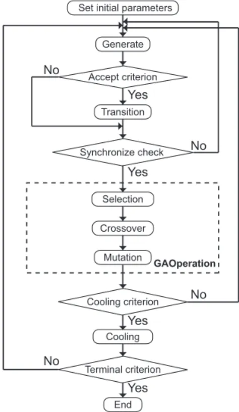
Set initial parameters
Generate
Transition Accept criterion
Synchronize check
Terminal criterion Cooling criterion
Cooling Selection Crossover Mutation
End
GAOperation
Yes Yes Yes Yes
No
No
No No
Figure 5: Algorithm of PSA/ANGA
criterion, and the transition of the solution are the same as conventional SA.
2. Neighborhood range is determined by GA
The synchronization of all the processes is done with a certain period, and the neighborhood ranges are determined by a GA based on the fitness value calculated from the energy of the solutions.
The neighborhood ranges of the multiple SA pro-
cesses are changed by crossover, mutation, and se-
lection. That is, the neighborhood ranges that gives
good solutions survive. Thus, all the neighborhood
ranges are expected to be converged to an appro-
priate neighborhood range for a problem.
The coding of the neighborhood range is repre- sented by the following equation.
N eighborhoodRange = M axRange · 10 X , (2) ( − 3 ≤ X ≤ 0) where X is the design variable and it is a 10-bit Grey coded binary. Therefore, the range of neighborhood can be very wide.
The 1-point crossover is used and the mutation is carried out by the 1-bit flip for the 10-bit string.
The crossover rate is 0.6.
3.3 Fitness value
The fitness values for the multiple neighborhood ranges for the selection of better neighborhood range are the minimum energies in multiple SA processes in the interval of the GA operations.
F itness = 1
Energy (3)
4 Numerical Experiments
4.1 Outline of experiments
To verify the validity and the effectiveness of the pro- posed method, PSA/ANGA, a parallel SA with opti- mum fixed neighborhood range, PSA/FN, a tempera- ture parallel SA, TPSA, and the TPSA with Corana’s adaptive neighborhood, TPSA/AN, are applied to solve three typical continuous optimization problems.
The parameters used are shown in Tables 3 and 4.
The number of neighborhood ranges is the same as the number of the SA processes. The maximum tempera- ture is determined so that the acceptance rate for the worst solutions becomes 0.5 in the preliminary experi- ment. The minimum temperature is determined accord- ing to the required accuracy[7].
Table 3: Parameters used for PSA/ANGA (Rastrigin, Griewank)
Function Rastrigin Griewank
Max.(Initial) temperature 10.0 20.0 Min.(Final) temperature 0.01 0.001
Cooling rate 0.8 0.726
Markov length 102400 307200
Synchronise cycle 1600 4800
Number of processors 32 32
For the TPSA, the temperatures are determined by the conventional method mentioned in [4], and the in- terval for exchange solutions are the same as the tem- perature change interval shown in Tables 3 and 4.
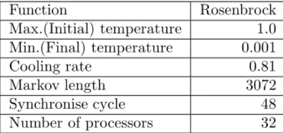
Table 4: Parameters used for PSA/ANGA (Rosenbrock)
Function Rosenbrock
Max.(Initial) temperature 1.0 Min.(Final) temperature 0.001
Cooling rate 0.81
Markov length 3072
Synchronise cycle 48
Number of processors 32
4.2 Parallel computer used
The parallel computer used is a PC cluster (Cambria cluster system) with 256 processor elements shown in Fig. 6, and 32 nodes are used for the experiments. The detail of the computer system is shown in Table 5.
Figure 6: PC cluster used
Table 5: Detail of the PC cluster used CPU Pentium3 800MHz(256CPU)
Memory 256MB × 256
Network FastEthernet OS Debian GNU/Linux 2.4
4.3 Experimental results
Figure 7 shows a typical example of the histories of the neighborhood ranges in 32 SA processes in solving the Rastrigin function. From this figure, it is found that the appropriate neighborhood range varies between 0.2 and 2 at the beginning, but it gradually decreases to around 0.1, and it finally converges to 0.01. That is, the appropriate neighborhood range varies from large to small, while the optimum fixed neighborhood range is 1.0.
Figure 8 shows a typical history of the neighborhood
range of the SA process that gives the best solution in
TPSA/AN. It can be seen that this type of adaptive
mechanism provides a very small neighborhood range
from the beginning, and the solution is trapped into
a local optimum. However, the TPSA alleviates this
problem since multiple SA processes with various tem-
peratures is running simultaneously and the solutions
Neighborhood range
10 -3 10 -2 10 -1 10 0 10 1
PSA/FN & TPSA/FN
Annealing steps ( 10000)
2
0 4 6 8 10
Figure 7: History of the neighborhood range in 32 SA process in solving the Rastrigin function
are interchanged among those SA processes, while sin- gle sequential SA with Corana’s adaptive neighborhood mechanism provides a local optimum at all times[7].
Neighborhood range
10 -3 10 -2 10 -1 10 0 10 1
Annealing steps ( 10000)
2
0 4 6 8 10
PSA/FN & TPSA/FN
Figure 8: History of the neighborhood range of the SA process that gives the best solution in TPSA/AN
For the Rastrigin function, the minimum neighbor- hood range to escape a local optimum is 1.0, there- fore the optimum fixed neighborhood range becomes 1.0. However, once the search region is within a global optimum region, the neighborhood range should be de- creased to obtain high accuracy. The proposed method can realize it. Furthermore, the population of the neigh- borhood ranges has a certain diversity as shown in Fig.
7, and the escape from a local minimum is easy.
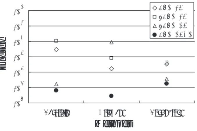
Figure 9 shows the performance of various methods.
These plots represent the median of 30 trials. The rea- son why the median is used is that the median is very reliable for comparing the converged energy values. The converged energy values sometimes vary in a wide range and the average value is affected by one extreme value.
From this figure, neither PSA/FN nor TPSA/FN give
Methods
Energy
㪩㪸㫊㫋㫉㫀㪾㫀㫅 㪞㫉㫀㪼㫎㪸㫅㫂 㪩㫆㫊㪼㫅㪹㫉㫆㪺㫂 㪧㪪㪘㪆㪝㪥 㪫㪧㪪㪘㪆㪝㪥 㪫㪧㪪㪘㪆㪘㪥 㪧㪪㪘㪆㪘㪥㪞㪘
Figure 9: Comparison of the converged energies
good performance in finding the minimum energy, while the proposed method, PSA/ANGA, provides the best performance of all. On the other hand, TPSA/AN pro- vides good performance for the Rastrigin and the Rosen- brock functions, but it does not give good performance for the Griewank function. This is due to the enormous local optima in the function.
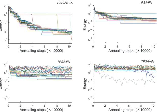
Figure 10 shows the typical histories of the energies of 32 SA processes. The proposed method, PSA/ANGA, shows fast decrease in the energy and very low minimum value, while other methods do not. In TPSA/FN and TPSA/AN, only the best history is effective, but, the best history does not outperform the result obtained by the proposed method. It can be seen that many other SA processes except for the best process do not greatly contribute in finding the optimum solution.
Consequently, the proposed mechanism for determin- ing the appropriate neighborhood by GA is found very effective, and PSA/ANGA can be considered to be a useful parallel SA method for continuous optimization.
It should be noted that the neighborhood range adap- tation mechanism adopted here can be realized with par- allel SA since the criterion for selecting good neigh- borhood range can be established from the relative value of the energies of the multiple SA processes. From this standpoint of view, parallelization of SA will give an- other new insight to optimization research field as well as speedup.
5 Conclusions
A new parallel simulated annealing method with adaptive neighborhood range mechanism is proposed here. The conclusions are as follows.
1. It is not easy to determine an appropriate neighbor- hood range for a continuous optimization problem in simulated annealing (SA).
2. The effect of the neighborhood range on the perfor-
mance of SA is investigated, and the appropriate
PSA/ANGA PSA/FN
TPSA/FN TPSA/AN
Annealing steps (10000)
Energy
10-6 10-4 10-2 100 102
Energy
10-6 10-4 10-2 100 102
Energy
10-6 10-4 10-2 100 102
Energy
10-6 10-4 10-2 100 102