An Application to El Bajo Espíritu Santo Seamount Near La Paz, Mexico

REGULAR ISSUE FEATURE

A PRACTICAL APPROACH TO MONITORING

MARINE PROTECTED AREAS

An Application to El Bajo Espíritu Santo Seamount Near La Paz, Mexico

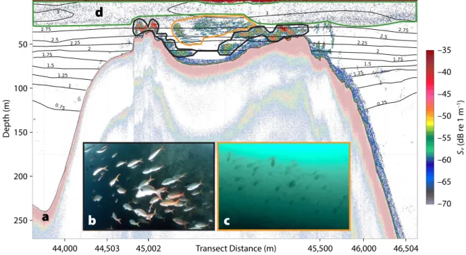
Some fish species observed at El Bajo Espíritu Santo Seamount are typical of rocky reefs in the Gulf of California. The larger blue fish are king angelfish (Holacanthus passer), and the smaller white fish are scissortail damselfish (Chromis atrilobata). Both species were pre- sumed to be too close to the seabed to be sampled acoustically.

By Héctor Villalobos, Juan P. Zwolinski, Carlos A. Godínez-Pérez, Violeta E. González-Máynez, Fernando Manini-Ramos, Melissa Mayorga-Martínez, William L. Michaels, Mitzi S. Palacios-Higuera,

Uriel Rubio-Rodríguez, Airam N. Sarmiento-Lezcano, and David A. Demer

INTRODUCTION

The creation of marine protected areas (MPAs) worldwide has outpaced the application of tools to monitor their marine resources and essential habitats and to preserve ecosystems to bolster fish production. Innovative approaches are needed to delineate and monitor MPAs using combined technologies to estimate fish abundances and distributions. The survey operations should simultaneously map and monitor other components of

the MPA ecosystem, such as zooplankton, oceanographic features, and seabed habi- tat. Acoustic-optical surveys (e.g., Demer, 2012; Michaels et al., 2019; Demer et al., 2020), using widely available instruments and software, offer a practical solution.

MPA waters might be surveyed period- ically using a scientific echosounder, a conductivity- temperature- depth probe (CTD), and underwater cameras deployed on the CTD and by scuba divers. The results could include descriptions of the

bathymetry, oceanographic habitat, dis- tributions of zooplankton and fishes, determination of the dominant fish spe- cies, and estimates of their biomasses.

An example of such an MPA sur- vey is one carried out at El Bajo Espíritu Santo Seamount (EBES). EBES is part of the MPA Parque Nacional Zona Marina del Archipielago de Espíritu Santo (PNZMAES), located in the south- west Gulf of California, Mexico, which together with other islands and pro- tected areas in the region is a UNESCO World Heritage Site (https://whc.unesco.

org/en/ list/ 1182). In 2007, PNZMAES was granted protected status to con- serve and protect its ecosystem, which is representative of islands in the Gulf of California (Secretaría de Medio Ambiente y Recursos Naturales, 2007).

The MPA is delineated by two rectan- gles, one around the archipelago and a smaller one around EBES ( ^{Figure 1} ).

While no-fishing areas are established within the larger rectangle, sportfishing and commercial fishing with handlines are permitted in most of the PNZMAES, which is the most productive area in the La Paz region (Hernández-Ortiz, 2013).

ABSTRACT. Worldwide, marine protected areas (MPAs) are increasingly created to protect and restore selected parts of the ocean and to enhance recreation, fishing, and sustainable resources. However, this process has outpaced the development and imple- mentation of methods for assessing and monitoring these habitats. Here, we combine data from an echosounder, a conductivity-temperature-depth probe, and underwater cameras to efficiently survey El Bajo Espíritu Santo Seamount, located in the southwest Gulf of California, Mexico. Results include a bathymetric map detailing a ridge with three peaks; oceanographic profiles showing a 35 m deep mixed layer and anoxic con- ditions below 200 m; mean target strength estimates for Pacific creolefish, Paranthias colonus (–34.8 dB re 1 m

, for mean total length ~33 cm), and finescale triggerfish, Balistes polylepis (–39.8 dB re 1 m

, 38 cm); baseline estimates of biomass for both spe- cies (55.7 t, 95% CI = 30.3–81.2 t and 38.9 t, 95% CI = 21.1–56.6 t, respectively) found only in the oxygenated water near the top of the seamount; and indications that these reef fishes grazed on zooplankton in the mixed layer. We conclude that acoustic- optical sampling is a practical approach for obtaining baseline information on MPAs and to efficiently monitor changes resulting from natural and anthropogenic processes.

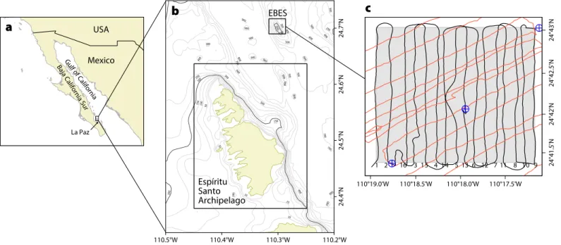
FIGURE 1. (a) Macrolocalization of the (b) Parque Nacional Zona Marina del Archipielago de Espíritu Santo (PNZMAES), with rectangles delineating the marine protected area (MPA), including the Espíritu Santo Archipelago and El Bajo Espíritu Santo Seamount (EBES). The coarse-scale bathymetry (GEBCO_2019) highlights the 200 m isobath (black). (c) At EBES, acoustic transects (black lines, numbered by transect) and CTD casts (blue symbols) were conducted on April 21, 2018. Red lines are acoustic sampling transects conducted on April 16, 2019.

Gulf of California Baja California Sur

La Paz

Mexico USA

Espíritu Santo Archipelago

110.4°W

110.5°W 110.3°W 110.2°W

24.4°N24.5°N24.6°N24.7°N

EBES

110°19.0'W 110°18.5'W 110°18.0'W 110°17.5'W

24°41.5'N24°42'N24°42.5'N24°43'N

1 2 16 3 15 4 14 5 13 6 12 7 11 8 10 9

a b c

From 2008 to 2009, 350 t to 500 t of fish were caught there (Comisión Nacional de Áreas Naturales Protegidas, 2014).

EBES is northeast of the Bay of La Paz, Baja California Sur, about 13 km north of the Espíritu Santo Archipelago ( ^{Figure 1} ).

It is a submarine ridge ~2.5 km long and

~0.8 km wide that rises from 1,000 m to ~18 m depth. Spring-tide currents

>0.5 m s

can cause twin eddies >1 km diameter in the lee (Klimley et al., 2005).

The area may also have cyclonic gyres, one observed with a 100 km diameter and an average west-periphery speed of 56 cm  s

(Emilsson and Alatorre, 1997). Mixing brings nutrients to the surface, promotes primary production, and aggregates plankton on the ridge.

The biomasses of plankton and macro- zooplankton exceed those at nearby sites (González-Armas et al., 2002; González- Rodríguez et  al., 2018). This produc- tion attracts reef fishes, pelagic fishes, and other vertebrates to the seamount (Klimley et  al., 2005) and makes EBES both ecologically and economically important (Klimley and Butler, 1988).

Transitions in the fish assemblage at EBES correspond with seasonal varia- tions in the Gulf of California hydrogra- phy (Robles and Marinone, 1987). During winter conditions (water temperature 16°–20°C), pelagic fishes at the seamount include mostly yellowtail, amberjack, and red snapper; during summer condi- tions (24°–26°C), there are green jacks, hammerhead sharks, dolphinfish, and yellow snapper (Klimley et al., 2005).

Hammerhead sharks routinely con-

gregate at EBES. A decline in their abun- dance (Klimley et al., 2005) corresponded to an increase in fishing for all hammer- head shark species worldwide during the past 50 years (Saldaña-Ruiz et al., 2017;

Gallagher and Klimley, 2018), and the likely extirpation of some species from the Gulf of California (Pérez-Jiménez, 2014). With the depletion of larger fishes, the fisheries diversified (Erisman et  al., 2010) and increasingly targeted Pacific creolefish (Paranthias colonus) and fine- scale triggerfish (Balistes polylepis) for human consumption rather than for fish bait (Sala et  al., 2003). Between 1998 and 2012, catches of these species in the PNZMAES each averaged ~10 t yr

(Hernández-Ortiz, 2013).

After more than a decade as an MPA, in November 2018 the PNZMAES became the first Mexican MPA to obtain the International Union for Conservation of Nature Green List Certificate, after meet- ing several criteria related to governance, design and planning, effective manage- ment, and conservation results (Ortega- Rubio et al., 2019). However, most of the

monitoring efforts focus on the archipel- ago, and the status and recovery of the ecosystem at EBES have yet to be assessed and monitored. Here, we demonstrate a practical acoustic-optical surveying method and provide information that may be useful to researchers and man- agers. First, we describe the collection of echosounder data for mapping bathym- etry and estimating the abundances of fish and zooplankton, as well as the col- lection of photographic images and video

to identify fish species. Next, we present a map of the seamount and estimates of target strengths and biomass for Pacific creolefish and finescale triggerfish. Then we discuss these results in the context of local hydrographic conditions, in partic- ular, the effect of dissolved oxygen on the vertical distribution of fish. Finally, we demonstrate how the integrated echo- sounder and optical sampling represents a cost-effective and practical approach for MPA monitoring.

METHODS Overview

Acoustic sampling was executed along equally spaced transects spanning the EBES rectangle in April 2018 and April 2019, following the guidelines in Simmonds and McLennan (2005). The seabed and fish with gas-filled swim- bladders created high-intensity echoes, indicating bathymetric features and fish- school locations, sizes, and densities, as described by Foote (1980). Plankton echoes were weaker but were of suffi- cient intensity to indicate their distri- bution and abundance, as in Hewitt and Demer (1991). The shapes of the fish and zooplankton aggregations, and bathymet- ric features, coupled with concurrently collected oceanographic information, allowed the separation and characteriza- tion of echoes from various taxa along the survey path. The identities of species contributing to the fish echoes were fur- ther refined using optical sampling with underwater cameras (e.g., Demer, 2012).

The densities of the most abundant spe- cies were estimated by dividing their summed echo intensities by their average echo energy, estimated for representa- tive animals (Simmonds and McLennan, 2005). Abundance was estimated by multiplying the average estimated fish density and the survey area. These steps are elaborated below.

Acoustic-Optical Survey

On April 21, 2018, the fishery research vessel BIP XII sampled 16 north- south parallel- line transects spaced 0.1 nmi

“ The work at EBES demonstrates that integrated

acoustic, optical, and environmental sampling can be

used to efficiently monitor fish populations and their

essential habitats at MPAs. ”

apart spanning the rectangular 2.6 nmi

EBES area ( ^{Figure 1} ) at an average speed of 6.5 kt. The survey was conducted during daytime hours, ending at sunset, 19:46 MDT. Transects 1–9 progressed from west to east, from 12:07 to 15:15, then interstitial transects 10–16 progressed from east to west, from 15:52 to 17:55.

Along the transects, acoustic back- scatter was measured with an echo- sounder (Simrad EK60) equipped with a 120 kHz split-beam transducer (Simrad ES120-7C) pole mounted port-side amid- ships, 3.19 m below the water surface.

Measurements were made using 1,024 μs duration sound pulses transmitted every 0.65 s. The acoustic data were indexed with time (GMT), geographic position, and ship speed; bearing data were mea- sured with a GPS receiver.

At the northeast and southwest cor- ners and center of the study area, a probe (SBE 19plus) was deployed to measure seawater salinity (S), temperature (T, °C), and dissolved oxygen (O

, mL L

) versus depth ( ^{Table 1} ).

During Cast 2, near the top of the seamount, an underwater video cam- era (GoPro Hero 4 Black Edition) was attached to the probe and deployed to 50  m depth. To minimize poten- tial reactions of fish to the probe, lights were not used. The images were exam- ined to identify the species that con- tributed to the concomitantly measured acoustic backscatter.

On the top of the seamount (24°42.069'N, 110°18.052'W), five scuba divers collected underwater video and photographic images to identify and count fish species and observe their behaviors.

The dives, to a maximum depth of 23.8 m, lasted 43 min with a “bottom time” of 36 min. The video cameras used during the dives were configured for 16 × 9 aspect, 1,920 × 1,080 pixels, 69.5° × 118.2° field of view, and 60 frames s

. To minimize potential reactions of fish to the divers, lights were used sparingly. Images were collected at depths ranging from 16.5 m to 23.8 m. The video-sampling dis- tance, ~12–14 m, was limited by depth

and water clarity. The photographic images (Nikon D500 camera and Sea &

Sea DY-D2J strobes, 5600 K) provided detailed images with correct color to bet- ter identify fish species. The images also provided relative estimates of fish length.

A 10 mm to 17  mm lens (Tokina) pro- vided a 100° × 180° field of view. The sam- pling range, ~5–8 m, was limited by the strobe illumination.

Because BIP XII had to divert around the dive boat, the shallowest portion of EBES was not sampled with the 120 kHz echosounder. Therefore, on April 16, 2019, the mapping of bathymetry on the top of EBES was completed using an echo- sounder (Simrad EK80 Portable) with a 38 kHz transducer (ES38-18). The 6 m long boat surveyed 12 transects spaced 0.1 nmi to 0.2 nmi, oriented southwest to northeast (60°) and vice versa (240°) ( ^{Figure 1} ). The 1,024 μs pulses were trans- mitted every 1.5–0.25 s, depending on the seabed depth.

Bathymetric Mapping

The 120 kHz data were analyzed using commercial software (Echoview v8), and the 38 kHz data were processed using open-source software (ESP3 v1.2.1;

Ladroit et al., 2020).

The mean temperature (14.7°C) and salinity (34.8) over 0 m to 280 m depth were used to estimate sound speed (1,525.24 m s

) (Fofonoff and Millard, 1983) and acoustic absorption at 120 kHz (0.048056 dB m

) and 38 kHz (0.006287 dB m

) (Francois and Garrison, 1982). The continuous noise power (≤–125 dB re 1 W) and tran- sient noise were removed (details in De Robertis and Higginbottom, 2007;

Ryan et al., 2015). For each transmission, the range to the seabed was estimated, indexed by date, time, and geographic position, and exported (.csv format).

The two bathymetry data sets were combined as overlapping data differed by

<1 m. Depth contours were interpolated on a 50 m grid using ordinary kriging (geoR; Ribeiro and Diggle, 2018) in R (R Core Team, 2020).

Hydrographic Characterization To obtain cross-sectional views of isolines spanning the area, the CTD data were interpolated using distances defined by variograms and correlograms. To iden- tify the water masses present in the sur- vey area, potential temperature and salin- ity versus depth were used to construct a T–S diagram. The anoxic depth was defined by a dissolved oxygen concentra- tion of <0.5 mL L

(Serrano, 2012).

Echo Classification

A –61 dB threshold on 120 kHz volume backscattering strength (S

; dB re 1 m

) was used to classify the echoes as either zooplankton (≤ –61 dB) or fish (> –61 dB).

The threshold was identified from itera- tive inspections of the distributions of S

within polygons drawn around echoes from aggregations of putative fish and then zooplankton ( ^{Figure 2} ).

To calculate the nautical area scatter- ing coefficients (s

; m

nmi

) for each taxon, the resulting zooplankton and fish echograms were each gridded into 3 m deep by 25 m long cells and depth- integrated. Results were mapped, the for- mer as interpolated contours (50 m grid) and the latter transformed to fish biomass (see Biomass Estimation below).

Target Strength Estimation

Using an algorithm with default param- eters (Echoview), target strength (dB re 1 m

) measurements of individual fish were obtained from the 120 kHz data collected at the location and time of CTD Cast 2. The echogram and video images from this period indicated aggregations

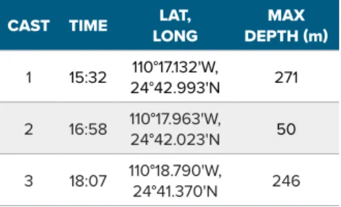
TABLE 1. Time, location, and depth of CTD casts.

CAST TIME LAT,

LONG MAX

DEPTH (m) 1 15:32 110°17.132'W,

24°42.993'N 271 2 16:58 110°17.963'W,

24°42.023'N 50 3 18:07 110°18.790'W,

24°41.370'N 246

of two predominant species above the top of the seamount. Boundaries were drawn around the data ( ^{Figure 2} ) close to the seabed (identified as Paranthias colonus in the images) and farther above it (Balistes polylepis), and target strength values for these regions were exported separately. To determine whether the data from these regions were represen- tative of fish atop other areas of the sea- mount, they were compared visually to the overall target strength distribution of single targets over the seamount. The mean target strength (TS) and corre- sponding mean backscattering cross sec- tions (σ

= 10

) for the two princi- pal species were calculated in the linear domain and assumed to be representative of all of the fish of the same species sur- veyed over the seamount.

Fish Mass Estimation

The distributions of total length (L

; cm) for each species of fish observed during the survey were assumed to be similar to those captured by fisherman at EBES from 2011 through 2017 (unpublished data from Sociedad de Historia Natural

Niparajá): for finescale triggerfish, root mean square total length (– L

) was 38 cm (24 ≤ L

≤ 50 cm), and for Pacific creole- fish, – L

was 33 cm (26 ≤ L

≤ 40 cm). These lengths were converted to mass (m; g) using the equation m = 0.0547 L

for triggerfish (Barroso-Soto et al., 2007) and m = 0.0547 L

for creolefish (Balart et al., 2006). The average mass per species is the arithmetic average of the individual mass estimates.

Biomass Estimation

For each grid cell, the s

attributed to fish was apportioned to each of the two pre- dominant species, Paranthias colonus and Balistes polylepis, using factors equal to the mean backscattering cross sec- tions measured for each species, and the backscatter- weighted proportion for that species, estimated from σ

and the num- ber of each species observed in the video.

For grid cells within the 200 m iso- bath, fish densities by species (fish nmi

) were calculated by dividing the nauti- cal area scattering coefficients by a fac- tor equal to the corresponding individual backscattering cross section multiplied by

D epth (m)

50

100

150

200

250

44,000 44,503 45,002 Transect Distance (m) 45,500 46,000 46,504 –35 –40 –45 –50 –55 –60 –65 –70

S

(dB r e 1 m

)

a b c

d

FIGURE 2. An example 120 kHz volume backscattering strength (S

) echogram for transect 5 (see Figure 1 for location), showing echoes from: (a) the seabed (red band), (b) Paranthias colonus (inside the black line), (c) Balistes polylepis (inside the orange line), and (d) zooplankton (inside the green line). The plot is overlaid with isolines of dissolved oxygen concentration (mL L

), calculated by Data-Interpolating Variational Analysis (Ocean Data View V.4; Schlitzer, 2015).

4π. Biomass densities (kg nmi

) for each species were calculated by multiplying these densities by the average-fish mass (kg fish

) for that species (Simmonds and MacLennan, 2005). These values, summed for both species and scaled to kg × 100 m

, were overlaid on a map of the depth contours and the interpolated zooplankton s

. Total biomass (B; t) was calculated for each species by multiplying the mean fish biomass density (t nmi

) by the area (nmi

) within the 200 m isobath.

The variance of the fish nautical area

scattering coefficient in the survey area

was calculated using geostatistical meth-

ods implemented in Estimation Variance

software (EVA; Petitgas and Prampart,

1995). A model was fit to the experi-

mental variogram of the mean fish den-

sity, which was then used to compute the

estimation variance of the mean biomass

taking into account the geometry of the

area, the length of the cell grid, the tran-

sect lengths, and the inter-transect dis-

tance (Petitgas, 1993). The standard error

of the mean biomass was used to approx-

imate the 95% confidence intervals (CIs)

for the biomass.

800 700 600

500 4 00

400 300

300 250

250

200 150 100 80 60

60 50

45 40 35

N

110°19.0'W 110°18.5'W 110°18.0'W 110°17.5'W

24°41.5 ' N 24°42.0 ' N 24°42.5 ' N 24°43.0 ' N

818 800 700 600 500 400 300 250 200 150 Depth (m)

100 80 60 50 45 40 35 30 25

FIGURE 3. Bathymetry throughout the El Bajo Espíritu Santo MPA. The ridge has three peaks, consistent with measurements by Klimley et al. (2005).

FIGURE 4. (a) Salinity, temperature, and dissolved oxygen versus depth at EBES, measured with three CTD casts conducted on April 21, 2018. The bot- tom of the mixed layer is at ~35 m depth, and the oxygen concentration is nearly anoxic (~0.5 mL L

) below ~200 m depth. (b) Water masses present at EBES on April 21, 2018, included Gulf of California Water (GCW), indicated by S > 35 and T > 12°C, and Subtropical Subsurface Water (SSW), indicated by 100 m < D < 500 m, 34.5 < S < 35.0 and 9.0° < T < 18.0°C (Torres-Orozco, 1993; Amador-Buenrostro et al., 2003). Not observed, but potentially in the area, were Equatorial Surface Water (ESW) characterized by 0 m < D < 100 m, S < 35, and T > 18.0°C, and Pacific Intermediate Water (PIW) characterized by D > 500 m, 34.5 < S < 34.8, and 4.0° < T < 9.0°C (Amador-Buenrostro et al., 2003).

300 250 200 150 100 50

0 12 14 16 18 20 22 Temperature (°C)

34.6 34.8 35.0 35.2 Salinity

0.5 1.0 1.5 2.0 2.5 3.0 Oxygen (mL L

)

Cast 1 Cast 2 Cast 3

Depth (m)

50 100 150 200 250

Depth (m)

34.6 34.8 35.0 35.2

12 14 16 18 20 22

Salinity

a b

Potential Temperature (°C) 26.5 26.0 25.5 25.0 24.5

24.0

27.0

ESW

SSW

GCW

σ 0

RESULTS Bathymetry

The bathymetry model for EBES indicates a shallow peak at ~25 m depth, and two deeper peaks at ~32 and ~43 m ( ^{Figure 3} ). To the west of the seamount the bottom depth exceeds 800 m, and to the east no more than 500 m. The ridge at the top of the seamount, defined here by the 200 m isobath, is about ~2.5 km long and ~0.8 km wide.

Oceanographic Environment

The CTD data indicate uniform conditions across EBES, with 34.6 < S < 35.3, 11° < T < 22.5°C, and 0.5 < O

< 3 mL L

. The high- est values for the three variables were found in the upper mixed layer.

Across the study site, the surface mixed layer was ~35 m deep. A sub- surface mixed layer, ~100 m to ~125 m depth, has S ~34.8, T ~14.5°C, and O

~0.75 mL L

. Casts 1 and 3 indicate nearly anoxic condi- tions (0.54 mL L

and 0.55 mL L

, respectively) at depths >200 m ( Figure 4a ).

During the survey, there were two predominant water-mass types at EBES ( ^{Figure 4b} ). Below the surface mixed layer, between

~25 m and ~70 m depths, the salty Gulf of California Water (GCW;

S ≥ 34.9, T ≥ 12.0°C; Torres-Orozco, 1993) results from evapora- tion of Equatorial Surface Water (ESW). Between depths of ~70 m and ~250 m, Subtropical Subsurface Water (SSW; 34.5 < S < 35.0;

9.0° ≤ T ≤ 18°C; Torres-Orozco, 1993) originates from the Pacific

Ocean (Castro et al., 2006).

Fish Species

Images from just one camera were used for identifying and counting fish to avoid overlap with imagery collected by the other four divers. Fish counts by species were estimated from 122 images, one from each 15 s segment of video. From these images, a total of 16 fish species were identified ( ^{Table 2} and Figure 5 ). The predominant species observed in the video, and more clearly identified in the still images are: Scissortail damsel- fish (Chromis atrilobata), Pacific creole fish (Paranthias colonus), yellowtail surgeonfish (Prionurus punctatus), finescale trigger- fish (Balistes polylepis), Cortez rainbow wrasse (Thalassoma lucasanum), and king angelfish (Holacanthus passer). Of these, P. colonus and B. polylepis accounted for 79.1% and 20.9% of the fish thought to be sufficiently above the seabed to be detected acoustically (see Demer et al., 2009). Though the fish were not measured, the still images taken during this study indicate that the B. polylepis were larger than the P. colonus.

FIGURE 5. Some fish species observed at EBES are typical of rocky reefs in the Gulf of California. (a) Aggregations of yellowtail surgeonfish (Prionurus punctatus) were feeding near the seabed on top of the sea- mount. This species was also presumed to be too close to the seabed to be sampled acoustically. Pacific creole fish (Paranthias colonus), which were generally observed farther off the seabed, are also shown. (b) Pacific creole fish (Paranthias colonus; orange tails), seen here schooling above the seabed near the top of the seamount, were the most common pelagic species observed by divers. (c) Finescale triggerfish (Balistes polylepis;

light color) were the second most common pelagic species observed by the divers. Mexican hogfish (Bodianus diplotaenia; black-spot stripes with yellow tail) were observed less frequently (see Table 2).

a

c b

TABLE 2. Number of individuals (n) and the species percentage observed (p) in 122 images. One image was extracted from each 15 s video segment collected during one scuba dive on the EBES seamount. Also indicated are the percentages of the two species that aggregated sufficiently above the reef to be sampled acoustically (P).

COMMON NAME SPECIES n p (%) P (%) Scissortail

damselfish

Chromis

atrilobata 1,174 42.77

Pacific creolefish Paranthias

colonus 681 24.82 79.1

Yellowtail surgeonfish

Prionurus

punctatus 305 11.11

Finescale

triggerfish Balistes

polylepis 180 6.56 20.9

Cortez rainbow wrasse

Thalassoma

lucasanum 179 6.52

King angelfish Holacanthus

passer 132 4.81

Barberfish Jhonrandalia

nigrirostris 33 1.20

Yellow snapper Lutjanus

argentiventris 15 0.55

Moray eel Gymnothorax spp. 14 0.51

Mexican hogfish Bodianus

diplotaenia 12 0.44

Cortez damselfish Stegastes

rectifraenum 6 0.22

Leopard grouper Mycteroperca

rosacea 5 0.18

Starry grouper Epinephelus

labriformis 4 0.15

Azure parrotfish Scarus

compressus 2 0.07

Large-banded

blenny Ophioblennius

steindachneri 2 0.07

Purple surgeonfish Acanthurus

xanthopterus 1 0.04

2,745 100.00

Target Strength

The target strength distribution shown in ^{Figure 6} largely includes measurements of individual Pacific creolefish and finescale triggerfish that were made throughout the survey. In addition, the distribution includes two small modes with higher values that may be from yellowtail surgeonfish (Prionurus punctatus) and king angelfish (Holacanthus passer), which were infrequently observed above the seabed ( ^{Table 2} ).

The mean target strength for in situ Pacific creolefish was –34.8 dB re 1 m

(σ

= 0.0003309 m

) (n = 141), assumed to correspond with – L

= 33 cm; and for in situ finescale triggerfish, mean target strength = –39.8 dB re 1 m

(σ

= 0.0001038 m

; n = 238; – L

= 38 cm) ( Figure 6 ).

Echo Classification and Biomass Estimation

The two dominant species of fish that were deemed sufficiently above the seabed to be detected acoustically were P. colonus (~79.1%) and B. polylepis (~20.9%) ( Table 2 ). Both spe- cies were assumed to contribute all of the fish acoustic back- scatter, nearly all of which (mean = 1,292 m

nmi

; max- imum = 63,002 m

nmi

) was near the top of the seamount, at depths <200 m, in seawater with dissolved oxygen concen-

FIGURE 6. Distribution of target strengths (dB re 1 m

) measured from all resolvable individual fish detected above the seamount (gray bars) and a fit probability density distribution (black line) compared to target strength distributions for Pacific creolefish (blue line) and finescale triggerfish (red line) concomitantly observed acoustically and optically during the second CTD cast. Based on their behaviors and numbers observed by the divers, the small third and fourth modes at ~ –29 dB and ~ –23 dB (arrow) may be from yellowtail surgeonfish (Prionurus punctatus) and king angelfish (Holacanthus passer).

Target Strength (dB re 1 m

)

Density

−50 −45 −40 −35 −30 −25 −20 −15

0.00 0.02 0.04 0.06 0.08 0.10 0.12

a b

FIGURE 7. Distributions of fish biomass density (blue circles), equaling the sum of estimates for P. colonus and B. polylepis for 25 m distances along the survey transects, and interpolated zooplankton backscatter in the 35 m deep surface layer (gray contours) for transects 1–9 (see Figure 1 for transect locations). The 200 m isobath (black), delimiting the biomass- estimation area, is distinguished from the other isobaths (white).

30 40 50 60 70 80

800 700

600 500

400

400 300

300 250

250

200 150 100 80

60 60 50

45 40 35

00 00 00 00 80

80 80 880 80 8 5 00 0 55

60 600000000 600000000 88888

8888

40000 40 4440 404000 40 40 40 40 40 440400400040 40 40440040040 4444 444440000000

600 660 60 60 60 60

0 00000 00 00 00 00 0 000 00 0 0 0 0 44

50 50 50 50 50 50 5 5

660 50

50 50 50500 50 50 50 5055500 50 50

6666666 666 666 66666 6 60 66 66 66 66 66 66 66 6 6 66 66 66 6 66 66 4

4 44 444 4 40 4 4 44 44 44 44 4 4444 44 44 44

000 6 66 6 6 6 6 44

44 4 44 0 5 44 4 0

0 55 50505005505000

50550500

20,000 10,000 5,000

110°19.0'W 110°18.5'W 110°18.0'W 110°17.5'W

24°41.5'N 24°42.0'N 24°42.5'N 24°43.0'N

s

(m

nmi

) kg × 100 m

tration >0.5 mL L

( Figure 2 ). The fish backscatter outside of this polygon was negligible (mean = 3.7 m

nmi

, maximum

= 461 m

nmi

). When converted to biomass, the maximum combined biomass densities were 23.15 t × 100 m

(mean = 475 kg × 100 m

) inside the polygon, and 169 kg × 100 m

(mean = 1.35 kg × 100

) in the remainder of the area. For the relatively oxygenated area within the 200 m isobath where most of the fish were observed, the estimates of total biomass are 55.7 t (95% CI = 30.3–81.2 t) for P. colonus (92% of total fish back- scatter), and 38.9 t (95% CI = 21.1–56.6 t) for B. polylepis (8%

of total fish backscatter) ( ^{Figure 7} ). The estimation variance was 95,021, and the coefficient of variation was 23.3%.

During the first pass, at midday, zooplankton backscatter was relatively homogeneously distributed throughout the MPA, mostly confined to the upper mixed layer ( ^{Figure 2} ), though it appeared to be lower above the top of the seamount ( ^{Figure 8a} ).

Considering only transects 1–9, the mean and maximum zoo-

plankton backscatter measures in the 35 m deep surface mixed

layer were 58 m

nmi

and 97 m

nmi

, respectively. In the sec-

ond acoustic pass, late in the day ( ^{Figure 8b} ), plankton back-

scatter increased toward the west. This pattern is attributed to

plankton migrating from deeper waters at the end of the day.

DISCUSSION

This study exemplifies the procedure for integrating acoustic, optical, and oceano- graphic data collection to cost-effectively survey and monitor a marine protected area. The echosounder, CTD, and camera sampling of the 2.6 nmi

EBES MPA was conducted during a ~7 hr period (exclud- ing travel time), but with refinements, the survey could either be completed in less time or expanded to cover the entire PNZMAES. This combination of sam- pling methods provided data to charac- terize the seabed and oceanographic hab- itats for pelagic fishes above the seamount and to identify the predominant species present and estimate their abundances.

The following sections provide a synopsis of the survey findings and suggestions for improving the efficiency and effectiveness of future surveys.

Bathymetry

Our bathymetric map of EBES ( ^{Figure 3} ) provides more detail than previously pub- lished maps, including that used to estab- lish the MPA (Comisión Nacional de Areas Naturales Protegidas, 2006). Other maps of the area are on larger scales (e.g., Klimley and Nelson, 1984; Amador- Buenrostro et  al., 2003) or their data sources and analysis methods are not

described (e.g.,  González-Armas et  al., 2002; Trasviña-Castro et al., 2003; Valle- Levinson et  al., 2004). A notable differ- ence between our bathymetry model and those of Klimley and Nelson (1984) and Amador-Buenrostro et  al. (2003) is the shallowest depth (25.5 m vs 18 m, respec- tively). This may be due to different loca- tions of the sampling transects, the grid- ding procedures and scales used, or both.

To resolve this discrepancy, a multibeam echosounder should be used to con- struct a comprehensive map of EBES bathymetry (Kenny et al., 2003).

Environment

The oceanographic characteristics of EBES have not been thoroughly defined (González-Rodríguez et  al., 2018), but seasonal variation is apparent (Klimley et al., 2005). During December to April, the sea surface temperature (SST) ranges from 19° to 24°C, and between May and November, it ranges from 25° to 29°C (Trasviña-Castro et al., 2003). During an El Niño event, SST tended towards the higher end of the latter range (Amador- Buenrostro et al., 2003). From July 2002 to April 2017, remotely sensed SST was lowest (~20°C) between February and March, and greatest (~30°C) during September to October (González-

Rodríguez et  al., 2018). Our measure- ments of SST during April (~22°C) are consistent with these published ranges of SST during spring.

During the transition from winter to summer conditions, the EBES area is increasingly stratified, and mixed layer depth decreases. Our measurements showed a 35 m deep mixed layer in April, compared to 20 m in June (Trasviña- Castro et  al., 2003) and 19 m in May (Verdugo-Díaz et  al., 2006). The salin- ity that we measured in the upper 100 m in April (34.8 to 35.3) is similar to that measured in the same area in June 1999 (Trasviña-Castro et al., 2003).

Our measurements of dissolved oxy- gen concentration may be the first pub- lished values for the EBES area. We observed a decrease in oxygen from

>2.5 mL L

above 50 m depth to

<1 mL L

at 100 m depth, and near hypoxic levels (~ 0.5 mL L

) deeper than 200 m. Throughout the Gulf of California, the depth of the oxygen mini- mum zone (OMZ) ranges from 100 m to 1,000 m (Hendrickx, 2001), and shoaling of the OMZ in the eastern Pacific may compress the potential habitat of marine organisms (Prince and Goodyear, 2006) compared to other areas in the world (Serrano, 2012).

FIGURE 8. Comparison of interpolated zooplankton acoustic density between transects (a) 1–9 and (b) 10–16 con- ducted on April 21, 2018. The first pass progressed from west to east, between 12:07 and 15:15 MDT, while the second pass progressed east to west from 15:52 to 17:55 MDT.

40 60 80 100 120 140

800 700

600

500 400

400 300

300 250

250

200 150 100 80 60

60 50

45 40 35

800 700

600

500 400

400 300

300 250

250

200 150 100 80 60

60 50

45 40 35

110°19.0'W 110°18.5'W 110°18.0'W 110°17.5'W 110°19.0'W 110°18.5'W 110°18.0'W 110°17.5'W

24°41.5'N 24°42.0'N 24°42.5'N 24°43.0'N s

(m

nmi

)

a b

Echo Classification

Because volume backscatter strength (S

) varies with scatterer type (e.g., size, shape, and material properties) and number per unit volume, its dependence on acous- tic wavelength or frequency is typically exploited to classify echoes. However, sev- eral methods have been used to thresh- old single-frequency S

from fish ver- sus plankton (e.g.,  López-Serrano et  al., 2018). Our empirical –61 dB threshold at 120 kHz is very close to that used in a study of small pelagic fish (–60.7 dB;

Gregg and Horne, 2009). Future sur- veys should include a lower frequency (e.g., 38 kHz) echosounder so the differ- ence in volume backscatter strength mea- sured at 120 kHz and 38 kHz may be used to better separate echoes from zooplank- ton and fish (Jech and Michaels, 2006).

Also, for fish biomass estimations, 38 kHz may provide more precise measures com- pared to higher frequencies.

Zooplankton

In our study, backscatter from zoo- plankton was predominantly in the upper mixed layer (<35 m depth) and was lowest over the top of the seamount ( ^{Figure 8a} ). During the early afternoon, the zooplankton backscatter decreased over the top of the bank and to the north- west, suggesting that the reef fish were grazing. Later in the day, the zooplank- ton backscatter increased due to the diel ascent of one or more unknown species, mostly from the deepest west side of the seamount ( ^{Figure 8b} ). Net samples could be used to identify the zooplankton spe- cies and sizes.

Species Identification

The 16 reef fish species identified in the images are common in the Gulf of California ( Table 2 ). Some of these species, for example, finescale trigger- fish and yellow snapper, may be found in the upper gulf (Walker, 1960), while all of them may be present at reefs south of Isla Tiburón in the central and lower gulf (Thomson et  al., 2000). All of these species have been observed at

Los Islotes, located north of Espíritu Santo Archipelago (Arreola-Robles and Elorduy-Garay, 2002) and previously at EBES (Rodríguez-Romero et  al., 2005).

Although the fish species at EBES change seasonally (Klimley et  al., 2005), year- round inhabitants may include reef fish such as scissortail damselfish, Pacific creolefish, and king angelfish (Rodríguez- Romero et  al., 2005), and pelagic fish such as yellow snapper and leopard grou- per (Jorgensen et al., 2016). We did not encounter pelagic fishes during our sur- vey of EBES in April.

Scissortail damselfish was the most con- spicuous and abundant species we found ( Table 2 ). Although its aggregations have been observed at depths ranging from the reef to the sea surface (Thomson et  al., 2000; Alvarez-Filip et al., 2006), we only observed damselfish schools near the sea- bed, where they are acoustically unresolv- able, so their biomass was not estimated.

Observations from the diver survey indi- cated schooling Pacific creolefish and finescale triggerfish close to the seafloor, but mostly swimming more than about 0.9 m above it and therefore acoustically resolvable. The acoustically unresolvable height above the seabed can be measured using multi-frequency split-beam echo- sounders (Demer et al., 2009).

Because reef fish may react to the pres- ence of divers, the estimated species pro- portions have some unknown observa- tional bias. Dickens et al. (2011) tried to quantify diver effects on reef fishes, and while they observed important declines in mean number of fish recorded, they con- cluded that underwater visual censuses are nonetheless a useful technique for estimating relative abundances. Seabed- mounted autonomous cameras may be used to mitigate any observational bias (Williams et al., 2014).

Fish Lengths

Landings data for EBES indicate that the total length of finescale triggerfish is gen- erally greater than that of Pacific creole- fish. The relative sizes observed in photo- graphic images from this study confirm

that finescale triggerfish were larger than Pacific creolefish at EBES in April 2018. Future surveys may include diver- operated stereo video that, in addition to species identification, could allow esti- mates of fish lengths (Goetze et al., 2015;

Demer et al., 2020).

Target Strengths

With the caveat that the echosounder was last calibrated approximately six years prior to this survey, this study produced the first published target strength measurements for in situ finescale triggerfish (mean tar- get strength = –39.8 dB re 1 m

) and in situ Pacific creolefish (mean target strength = –34.8 dB re 1 m

). Using a common tar- get strength versus length relationship (target strength = 20 log

(L

(cm)) + b

) and the root mean square total length values, the reduced target strength was b

= –65.2 dB for in situ Pacific creole- fish and b

= –71.4 dB for in situ fines- cale triggerfish. These values are similar to those suggested by Foote (1987) for physo- clists (–67.4 dB) and clupeoids (–71.9 dB).

Note that the calibration does not affect the conversion of area backscattering coefficients to fish densities using the in situ average target strength because both sources of data were collected with the same instrument.

Fish Biomass

For EBES in April 2018, our estimate of Pacific creolefish biomass is 55.7 t (95% CI = 30.3–81.2 t), which is about 40% higher than that of finescale trigger- fish (38.9 t, 95% CI = 21.1–56.6 t). These estimates may be negatively biased due to the unsampled fish aggregations located close to the seabed. While fishery data for the EBES area are scarce, our biomass estimates are plausible given the 10 t yr

average catch of each species within the larger archipelago rectangle.

Recommendations

All of the observed reef fishes were shal-

lower than ~200 m depth within oxy-

genated water. If the OMZ depth is static

or shoals, future surveys of reef fishes at

EBES could be constrained to the area within the 200 m isobath. Transects with smaller spacing, oriented perpendicu- lar to the bathymetric contours, could reduce the estimation variance. More CTD casts with video cameras could be deployed along the ridge to better iden- tify and enumerate the species of fish present and improve the characterization of their oceanographic habitat.

CONCLUSION

The work at EBES demonstrates that integrated acoustic, optical, and envi- ronmental sampling can be used to effi- ciently monitor fish populations and their essential habitats at MPAs. These technologies provide information from depths not accessible to divers. As a specific example, this study provided the most detailed bathymetric map of EBES to date, revealing a 2.5 km long and 0.8  km wide seamount with three peaks. It showed that salinity, tempera- ture, and oxygen profiles were stratified across EBES and the mixed layer was

~35 m deep, both signaling a transitional state between winter and summer condi- tions. The measures of dissolved oxygen concentration at EBES, perhaps the first published values, indicate anoxic condi- tions below ~200 m deep. Zooplankton backscatter was mostly in the upper mixed layer and fish backscatter was in oxygenated water. Zooplankton den- sity decreased throughout the afternoon, hypothetically due to grazing, and then increased in the evening, apparently due to diel vertical migration of one or more unknown species. Pacific creole- fish and finescale triggerfish were the predominant species of schooling reef fish, with estimated biomasses of 55.7 t (95% CI = 30.3–81.2 t) and 38.9 t (95% CI

= 21.1–56.6 t), respectively. These results may serve as a baseline for managers to monitor the recoveries of fish stocks at EBES (Nash and Graham, 2016) and for researchers to continue studying this MPA ecosystem.

REFERENCES

Alvarez-Filip, L., H. Reyes-Bonilla, and L.E. Calderon- Aguilera. 2006. Community structure of fishes in Cabo Pulmo reef, Gulf of California. Marine Ecology 27(3):253–262, https://doi.org/ 10.1111/

j.1439-0485.2006.00108.x.

Amador-Buenrostro, A., A. Trasviña-Castro, A. Muhlia- Melo, and M.L. Argote-Espinoza. 2003. Influence of EBES seamount and Farallon basin on coastal cir- culation in the Gulf of California, Mexico. Geofísica Internacional 42(3):407–418.

Arreola-Robles, J.L., and J.F. Elorduy-Garay. 2002.

Reef fish diversity in the region of La Paz, Baja California Sur, Mexico. Bulletin of Marine Science 70(1):1–18.

Balart, E.F., A. González-Cabello, R.C. Romero-Ponce, A. Zayas-Alvarez, M. Calderón-Parra, L. Campos- Dávila, and L.T. Findley. 2006. Length-weight rela- tionships of cryptic reef fishes from the southwest- ern Gulf of California, Mexico. Journal of Applied Ichthyology 22:316–318.

Barroso-Soto, I., E. Castillo-Gallardo, C. Quiñonez- Velázquez, and R.E. Morán-Angulo. 2007.

Age and growth of the finescale triggerfish, Balistes polylepis (Teleostei: Balistidae), on the coast of Mazatlán, Sinaloa, Mexico. Pacific Science 61:121–127, https://doi.org/10.1353/

psc.2007.0002.

Castro, R., R. Durazo, A. Mascarenhas, C.A. Collins, and A. Trasviña. 2006. Thermohaline variability and geostrophic circulation in the southern por- tion of the Gulf of California. Deep Sea Research Part I 53(1):188–200, https://doi.org/10.1016/

j.dsr.2005.09.010.

Comisión Nacional de Áreas Naturales Protegidas.

2006. Estudio Previo Justificativo para el esta- blecimiento del Área Natural Protegida “Parque Nacional Espíritu Santo.” México, D.F.

Comisión Nacional de Áreas Naturales Protegidas.

2014. Programa de Manejo. Parque Nacional exclusivamente la zona marina del Archipiélago de Espíritu Santo. SEMARNAT, México, D.F., 233 pp.

Demer, D.A., G.R. Cutter, J.S. Renfree, and J.L. Butler. 2009. A statistical-spectral method for echo classification. ICES Journal of Marine Science 66:1,081–1,090, https://doi.org/10.1093/

icesjms/fsp054.

Demer, D.A. 2012. 2007 Survey of Rockfishes in the Southern California Bight Using the Collaborative Optical-Acoustic Survey Technique. Technical report, NOAA-TM-NMFS-SWFSC-498, 110 pp.

Demer, D.A., W.L. Michaels, T. Algrøy, L.N. Andersen, O. Abril-Howard, B. Binder, D. Bolser, R. Caillouet, M.D. Campbell, S. Cambronero-Solano, and others.

2020. Integrated Optic-Acoustic Studies of Reef Fish: Report of the 2018 GCFI Field Study and Workshop. NMFS-F/SPO-208, 61 pp.

De Robertis, A., and I. Higginbottom. 2007.

A post-processing technique to estimate the signal- to- noise ratio and remove echosounder background noise. ICES Journal of Marine Science 64:1,282–1,291, https://doi.org/10.1093/

icesjms/fsm112.

Dickens, L.C., C.H.R. Goatley, J.K. Tanner, and D.R. Bellwood. 2011. Quantifying relative diver effects in underwater visual censuses. PLoS ONE 6(4):e18965, https://doi.org/10.1371/journal.

pone.0018965.

Emilsson, I., and M. Alatorre. 1997. Evidencias de un remolino ciclónico de mesoescala en la parte sur del Golfo de California. Pp. 173–182 in Contribuciones a la Oceanografía Física en México. M.F. Lavín, ed, Monografía 3, Unión Geofísica Mexicana.

Erisman, B., I. Mascarenas, G. Paredes, Y. Sadovy de Mitcheson, O. Aburto-Oropeza, and P. Hastings.

2010. Seasonal, annual, and long-term trends in commercial fisheries for aggregating reef fishes in the Gulf of California, Mexico. Fisheries Research 106(3):279–288, https://doi.org/10.1016/

j.fishres.2010.08.007.

Fofonoff, N.P., and R. Millard Jr. 1983. Algorithms for the computation of fundamental properties of seawater. UNESCO Technical Papers in Marine Science 44:53.

Foote, K.G. 1980. Importance of the swimbladder in acoustic scattering by fish: A comparison of gadoid and mackerel target strengths. The Journal of the Acoustical Society of America 67(6):2084, https://doi.org/ 10.1121/1.384452.

Foote, K.G. 1987. Fish target strengths for use in echo integrator surveys. The Journal of the Acoustical Society of America 82(3):981, https://doi.org/ 10.1121/

1.395298.

Francois, R., and G. Garrison. 1982. Sound absorp- tion based on ocean measurements: Part II. Boric acid contribution and equation for total absorp- tion. The Journal of the Acoustical Society of America 72(6):1879, https://doi.org/10.1121/1.388673.

Gallagher, A.J., and A.P. Klimley. 2018. The biol- ogy and conservation status of the large hammer- head shark complex: The great, scalloped, and smooth hammerheads. Reviews in Fish Biology and Fisheries 28(4):777–794, https://doi.org/10.1007/

s11160-018-9530-5.

Goetze, J.S., S.D. Jupiter, T.J. Langlois, S.K. Wilson, E.S. Harvey, T. Bond, and W. Naisilisili. 2015. Diver operated video most accurately detects the impacts of fishing within periodically harvested closures. Journal of Experimental Marine Biology and Ecology 462:74–82, https://doi.org/10.1016/

j.jembe.2014.10.004.

González-Armas, R., R. Palomares-García, and R. De Silva-Dávila. 2002. Copepod and macrozoo- plankton distribution associated to El Bajo Espíritu Santo Seamount. Pp. 183–193 in Contribution to the Study of East Pacific Crustaceans. M.E. Hendrickx, ed, Instituto de Ciencias del Mar y Limnología, UNAM, México.

González-Rodríguez, E., A. Trasviña-Castro, and A. Ramos-Rodríguez. 2018. El Bajo de Espíritu Santo; punto caliente de abundancia biológica afuera de Bahía de La Paz. CICIMAR Oceánides 33(1):13–24, https://doi.org/10.37543/

oceanides.v33i1.224.

Gregg, M.C., and J.K. Horne. 2009. Turbulence, acoustic backscatter, and pelagic nekton in Monterey Bay. Journal of Physical

Oceanography 39(5):1,097–1,114, https://doi.org/

10.1175/2008JPO4033.1.

Hendrickx, M.E. 2001. Occurrence of a continental slope decapod crustacean community along the edge of the minimum oxygen zone in the south- eastern Gulf of California, Mexico. Belgian Journal of Zoology 131(suppl. 2):95–109.

Hernández-Ortiz, D.X. 2013. Evaluación de la efec- tividad del Parque Nacional Zona Marina del Archipiélago Espíritu Santo como herramienta de conservación y generación de beneficios socio- económico. BSc Thesis, Universidad Autónoma de Baja California Sur, La Paz, BCS, México.

Hewitt, R., and D. Demer. 1991. Krill abundance.

Nature 353:310, https://doi.org/10.1038/353310b0.

Jech, J.M., and W.L. Michaels. 2006. A multifrequency method to classify and evaluate fisheries acoustics data. Canadian Journal of Fisheries and Aquatic Sciences 63(10):2,225–2,235, https://doi.org/

10.1139/F06-126.

Jorgensen, S.J., A.P. Klimley, A. Muhlia-Melo, and S.G. Morgan. 2016. Seasonal changes in fish assemblage structure at a shallow seamount in the Gulf of California. PeerJ 4:e2357, https://doi.org/

10.7717/peerj.2357.

Kenny, A.J., I. Cato, M. Desprez, G. Fader, R. Schüttenhelm, and J. Side. 2003. An over- view of seabed-mapping technologies in the con- text of marine habitat classification. ICES Journal of Marine Science 60(2):411–418, https://doi.org/

10.1016/ S1054-3139(03)00006-7.

Klimley, A.P., and D.R. Nelson. 1984. Diel move-

ment patterns of the scalloped hammerhead

shark (Sphyrna lewini) in relation to El Bajo Espíritu

Santo: A refuging central-position social system.

Behavioral Ecology and Sociobiology 15(1):45–54, https://doi.org/10.1007/BF00310214.

Klimley, A.P., and S. Butler. 1988. Immigration and emi- gration of a pelagic fish assemblage to seamounts in the Gulf of California related to water mass movements using satellite imagery. Marine Ecology Progress Series 49(1):11– 20, https://doi.org/

10.3354/ meps049011.

Klimley, A.P., J.E. Richert, and S.J. Jorgensen. 2005.

The home of blue water fish: Rather than singly inhabiting the trackless ocean, pelagic fish spe- cies travel together in groups, which migrate between hidden, productive oases. American Scientist 93(1):42–49.

Ladroit, Y., P.C. Escobar-Flores, A.C.G. Schimel, and R.L. O’Driscoll. 2020. ESP3: An open-source software for the quantitative processing of hydro-acoustic data. SoftwareX 12(2020):100581, https://doi.org/10.1016/j.softx.2020.100581.

López-Serrano, A., H. Villalobos, and M.O. Nevárez- Martínez. 2018. A probabilistic procedure for esti- mating an optimal echo-integration threshold using the Expectation-Maximisation algorithm. Aquatic Living Resources 31:12, https://doi.org/10.1051/

alr/2017048.

Michaels, W.L., B. Binder, K. Boswell, L.M. Chérubin, D.A. Demer, T. Jarvis, F.R. Knudsen, C. Lang, J.E. Paramo, P.J. Sullivan, and others. 2019. Best Practices for Implementing Acoustic Technologies to Improve Reef Fish Ecosystem Surveys: Report from the 2017 GCFI Acoustics Workshop. NOAA Technical Memo NMFS-F/SPO-192, 161 pp., https://spo.nmfs.noaa.gov/sites/default/files/

TM192.pdf.

Nash, K.L., and N.A. Graham. 2016. Ecological indica- tors for coral reef fisheries management. Fish and Fisheries 17(4):1,029–1,054, https://doi.org/10.1111/

faf.12157 .

Ortega-Rubio, A., I. González-López, I. March- Mifsut, E.I. Bustamante-Moreno, M.Á. Palmeros- Rodríguez, N. Bojórquez-Galeana, A. Suárez, and B. Bermúdez-Almada. 2019. Parque Nacional Zona Marina del Archipiélago Espíritu Santo: Primer Área Natural Protegida de México con el Certificado Lista Verde de UICN. Áreas Naturales Protegidas Scripta 5(1):43–68.

Pérez-Jiménez, J.C. 2014. Historical records reveal potential extirpation of four hammerhead sharks (Sphyrna spp.) in Mexican Pacific waters. Reviews in Fish Biology and Fisheries 24(2):671–683, https://doi.org/10.1007/s11160-014-9353-y.

Petitgas, P. 1993. Geostatistics for fish stock assess- ments: A review and an acoustic application.

ICES Journal of Marine Science 50(3):285–298, https://doi.org/10.1006/jmsc.1993.1031.

Petitgas, P., and A. Prampart. 1995. EVA Estimation VAriance: logiciel de géostatistique pour l’analyse structurale et les calculs de variance. ORSTOM.

Prince, E.D., and C.P. Goodyear. 2006. Hypoxia- based habitat compression of tropical pelagic fishes. Fisheries Oceanography 15(6):451–464, https://doi.org/ 10.1111/j.1365-2419.2005.00393.x.

R Core Team. 2020. R: A Language and Environment for Statistical Computing. R Foundation for Statistical Computing, Vienna, Austria.

Ribeiro, P.J. Jr., and P.J. Diggle. 2018. geoR: Analysis of Geostatistical Data. R package version 1.7-5.2.1.

Robles, J.M., and S.G. Marinone. 1987. Seasonal and interannual thermohaline variability in the Guaymas Basin of the Gulf of California. Continental Shelf Research 7(7):715–733, https://doi.org/ 10.1016/

0278-4343(87)90013-6.

Rodríguez-Romero, J., A.F. Muhlia-Melo, F. Galván- Magaña, F.J. Gutiérrez-Sánchez, and V. Gracia- López. 2005. Fish assemblages around Espíritu Santo island and Espíritu Santo Seamount in the lower Gulf of California, Mexico. Bulletin of Marine Science 77(1):33–50.

Ryan, T.E., R.A. Downie, R.J. Kloser, and G. Keith. 2015.

Reducing bias due to noise and attenuation in open-ocean echo integration data. ICES Journal of Marine Science 72(8):2,482–2,493, https://doi.org/

10.1093/ icesjms/fsv121.

Sala, E., O. Aburto-Oropeza, G. Paredes, and G. Thompson. 2003. Spawning aggregations and reproductive behavior of reef fishes in the Gulf of California. Bulletin of Marine Science 72(1):103–121.

Saldaña-Ruiz, L.E., O. Sosa-Nishizaki, and D. Cartamil.

2017. Historical reconstruction of Gulf of California shark fishery landings and species composition, 1939–2014, in a data-poor fishery context. Fisheries Research 195:116–129, https://doi.org/10.1016/

j.fishres.2017.07.011.

Schlitzer, R. 2015. Ocean Data View User’s Guide.

Alfred Wegener Institute, Bremerhaven, Germany, 150 pp.

Secretaría de Medio Ambiente y Recursos Naturales.

2007. Decreto por el que se declara área natu- ral protegida, con la categoría de Parque Nacional exclusivamente la zona marina del Archipiélago de Espíritu Santo, ubicado en el Golfo de California, frente a las costas del Municipio de La Paz, Baja California Sur. Diario Oficial de la Federación, 10 de mayo de 2007. Primera sección. México.

Serrano, D. 2012. La zona del mínimo de oxígeno en el Pacífico mexicano. Pp. 105–119 in Biodiversidad y comunidades del talud continental del Pacífico mexicano. P. Zamorano, M.E. Hendrickx, and M. Caso, eds, Secretaría del Medio Ambiente y Recursos Naturales, Instituto Nacional de Ecología.

Simmonds, E.J., and D.N. MacLennan. 2005. Fisheries Acoustics: Theory and Practice. Blackwell, Oxford, 456 pp.

Thomson, D.A., L.T. Findley, and A.N. Kerstitch. 2000.

Reef Fishes of the Sea of Cortez: The Rocky-Shore Fishes of the Gulf of California, Revised edition.

University of Texas Press, Austin, Texas, 407 pp.

Torres-Orozco, E. 1993. Análisis volumétrico de las masas de agua del Golfo de California.

MSc Thesis, Centro de Investigación Científica y Educación Superior de Ensenada (CICESE), Ensenada, B.C., México.

Trasviña-Castro, A., G. Gutierrez de Velasco, A. Valle- Levinson, R. González-Armas, A. Muhlia, and M. Cosio. 2003. Hydrographic observations of the flow in the vicinity of a shallow seamount top in the Gulf of California. Estuarine, Coastal and Shelf Science 57(1-2):149–162, https://doi.org/10.1016/

S0272-7714(02)00338-4.

Valle-Levinson, A., A. Trasviña-Castro, G. Gutiérrez de Velasco, and R. González-Armas. 2004.

Diurnal vertical motions over a seamount of the southern Gulf of California. Journal of Marine Systems 50(1–2):61–77.

Verdugo-Díaz, G., R. Cervantes-Duarte, and M.O. Albañez-Lucero. 2006. Variación estacio- nal de la productividad primaria estimada por fluo- rescencia natural en El Bajo Espíritu Santo, BCS, México. Naturaleza y Desarrollo 4(2):35–40.

Walker, B.W. 1960. The distribution and affinities of the marine fish fauna of the Gulf of California.

Systematic Zoology 9(3/4):123–133, https://doi.org/

10.2307/2411961.

Williams, K., A. De Robertis, Z. Berkowitz, C. Rooper, R. Towler. 2014. An underwater stereo-camera trap.

Methods in Oceanography 11:1–12, https://doi.org/

10.1016/j.mio.2015.01.003.

DISCLAIMER

This publication does not approve, recommend, or endorse any proprietary product or proprietary mate- rial mentioned herein, or which has as its purpose an intent to cause directly or indirectly the adver- tised product to be used or purchased because of this publication.

ACKNOWLEDGMENTS

The survey and data analyses for this study were con- ducted during a one-week “Workshop on Acoustic- Optical Surveys,” funded by the NOAA Fisheries Advanced Sampling Technologies Program, and hosted at CICIMAR-IPN in La Paz, BCS, Mexico (April 20–27, 2018). Cesar Salinas-Zavala and Eduardo Balart (CIBNOR, SC) contributed BIP XII ship time for the survey. Lars N. Andersen (SIMRAD) and Toby Jarvis (Echoview) provided remote assistance and instruction to Mexican participants. Leonardo Figueroa-Albornoz (Kongsberg Mexico) assisted with logistics during the survey. José Manuel Borges- Souza (CICIMAR-IPN) guided the dive. The EK80 Portable used for collecting bathymetry data in April 2019 was lent by Kongsberg Maritime as part of a testing program for a low-cost scientific echo- sounder suitable for shallow water work across a wide range of applications. To enable his participa- tion in this work, HV received grants from the SNI (CONACYT), and COFAA and EDI programs from IPN.

AUTHORS

Héctor Villalobos ([email protected]) is Research Scientist, Instituto Politécnico Nacional, Centro Interdisciplinario de Ciencias Marinas (CICIMAR-IPN), La Paz, Baja California Sur (BCS), Mexico. Juan P. Zwolinski is Research Associate, University of California, Santa Cruz, affiliated with NOAA Southwest Fisheries Science Center, La Jolla, CA, USA. Carlos A. Godínez-Pérez is an MsC student, CICIMAR-IPN, La Paz, BCS, Mexico.

Violeta E. González-Máynez is Research Scientist, Instituto Nacional de Pesca y Acuacultura, CRIAP Unidad Guaymas, Guaymas, Sonora, Mexico.

Fernando Manini-Ramos is Field Technician, Centro de Investigaciones Biológicas del Noroeste (CIBNOR, SC), La Paz, BCS, Mexico.

Melissa Mayorga-Martínez is a PhD student, Instituto de Ciencias Marinas y Pesquerías, Universidad Veracruzana, Boca del Río, Veracruz, Mexico. William L. Michaels is Research Scientist, National Oceanic and Atmospheric Administration, Office of Science and Technology, Silver Spring, MD, USA. Mitzi S. Palacios-Higuera is Field Technician, CIBNOR, SC, La Paz, BCS, Mexico.

Uriel Rubio-Rodríguez is a PhD student, CICIMAR- IPN, La Paz, BCS, Mexico, currently at Universidad del Valle de México, Departamento de Ciencias de la Salud. Airam N. Sarmiento-Lezcano is an MsC student, CICIMAR-IPN, currently at Instituto de Oceanografía y Cambio Global, Universidad de Las Palmas de Gran Canaria, Unidad Asociada ULPGC-CSIC, Campus de Taliarte, Gran Canaria, Canary Islands, Spain. David A. Demer is Senior Scientist, NOAA Southwest Fisheries Science Center, La Jolla, CA, USA.

ARTICLE CITATION

Villalobos, H., J.P. Zwolinski, C.A. Godínez-Pérez, V.E. González-Máynez, F. Manini-Ramos, M. Mayorga- Martínez, W.L. Michaels, M.S. Palacios-Higuera, U. Rubio-Rodríguez, A.N. Sarmiento-Lezcano, and D.A. Demer. 2021. A practical approach to moni- toring marine protected areas: An application to El Bajo Espíritu Santo Seamount near La Paz, Mexico.

Oceanography 34(3):32–43, https://doi.org/10.5670/

oceanog.2021.303.

COPYRIGHT & USAGE

This is an open access article made available under the terms of the Creative Commons Attribution 4.0 International License (https://creativecommons.org/

licenses/by/4.0/), which permits use, sharing, adapta-

tion, distribution, and reproduction in any medium or

format as long as users cite the materials appropri-

ately, provide a link to the Creative Commons license,

and indicate the changes that were made to the

original content.