Impacts of international transport
infrastructure: evidence from Laos households
著者 Magnus Andersson, Hayakawa Kazunobu, Souknilanh Keola, Yamanouchi Kenta 権利 Copyrights 2021 by author(s)
journal or
publication title
IDE Discussion Paper
volume 812
year 2021‑03
URL http://hdl.handle.net/2344/00052038
INSTITUTE OF DEVELOPING ECONOMIES
IDE Discussion Papers are preliminary materials circulated to stimulate discussions and critical comments
* Deputy Director, Economic Geography Studies Group, Development Studies Center, IDE ([email protected])
IDE DISCUSSION PAPER No. 812
Impacts of International Transport Infrastructure: Evidence from Laos Households
Magnus ANDERSSON, Kazunobu HAYAKAWA, Souknilanh KEOLA*, and Kenta YAMANOUCHI
March 2021
Abstract: This study investigates the impact of international transport infrastructure on household living standards. We propose that a change in the share of food expenditure to total expenditure is a valid indicator of the improvement in living standards by infrastructure in developing countries. We apply this notion to the case of an international bridge between Laos and Thailand and explore its effects on Laos households. Our estimation results by difference-in-differences analysis and propensity score matching method show that establishing an international bridge decreases the share of food expenditure, suggesting that the living standards of the households close to the bridge were improved. Our main results are robust to alternative treatment measurements. Finally, we explored the heterogeneity of the treatment effects using a machine learning approach. We found that although the initial level of the total expenditure affected households’ ability to benefit from the bridge, all households, regardless of their characteristics, could benefit if they were in the districts close to the bridge.
Keywords: International bridge; Trade liberalization; Household JEL Classification: F10, H54, G51
The Institute of Developing Economies (IDE) is a semigovernmental, nonpartisan, nonprofit research institute, founded in 1958. The Institute merged with the Japan External Trade Organization (JETRO) on July 1, 1998.
The Institute conducts basic and comprehensive studies on economic and related affairs in all developing countries and regions, including Asia, the Middle East, Africa, Latin America, Oceania, and Eastern Europe.
The views expressed in this publication are those of the author(s). Publication does not imply endorsement by the Institute of Developing Economies of any of the views expressed within.
INSTITUTE OF DEVELOPING ECONOMIES (IDE), JETRO 3-2-2, WAKABA,MIHAMA-KU,CHIBA-SHI
CHIBA 261-8545, JAPAN
©2021 by author(s)
No part of this publication may be reproduced without the prior permission of the author(s).
1
Impacts of International Transport Infrastructure:
Evidence from Laos Households
§Magnus ANDERSSON
Department of Urban Studies, Malmö University, Sweden
Kazunobu HAYAKAWA
Development Studies Center, Institute of Developing Economies, Japan
Souknilanh KEOLA
Development Studies Center, Institute of Developing Economies, Japan
Kenta YAMANOUCHI#
Faculty of Economics, Kagawa University, Japan
Abstract: This study investigates the impact of international transport infrastructure on household living standards. We propose that a change in the share of food expenditure to total expenditure is a valid indicator of the improvement in living standards by infrastructure in developing countries. We apply this notion to the case of an international bridge between Laos and Thailand and explore its effects on Laos households. Our estimation results by difference-in-differences analysis and propensity score matching method show that establishing an international bridge decreases the share of food expenditure, suggesting that the living standards of the households close to the bridge were improved. Our main results are robust to alternative treatment measurements. Finally, we explored the heterogeneity of the treatment effects using a machine learning approach. We found that although the initial level of the total expenditure affected households’ ability to benefit from the bridge, all households, regardless of their characteristics, could benefit if they were in the districts close to the bridge.
Keywords: International bridge; Trade liberalization; Household JEL Classification: F10, H54, G51
1. Introduction
Improving transport infrastructure is key in facilitating economic transactions. Well- functioning infrastructure facilitates fast and secure delivery and, therefore, lowers transport costs. Building a new high-quality infrastructure is essential, especially in developing countries, as these countries usually rely on relatively fragile facilities for
§ We would like to thank Kyoji Fukao, Satoru Kumagai, and the seminar participants in the Institute of Developing Economies for their invaluable comments. This work was supported by JSPS KAKENHI Grant Number #18KK0050 and #17K03751. All remaining errors are ours.
# Corresponding author: Souknilanh Keola; Address: 3-2-2, Wakaba, Mihama-ku, Chiba-shi, Chiba 261- 8545, Japan. Tel: 81-43-299-9500; E-mail: [email protected].
2
transport. Thus, local prices of goods are completely different, both within and between countries. The difference in prices motivates economic transactions and implies potential gains from trade. Constructing an effective infrastructure, therefore, helps economic development and improvement in the living standards in developing countries by reducing transport costs and converging local prices across countries or regions.
In this study, we focus on the construction of an international transport infrastructure for households in a developing country. We demonstrate that a change in the share of food expenditure from total expenditure is a valid indicator of the improvement in living standards in developing countries as the local price differs across locations, and the effects of the transport infrastructure on transport cost would vary significantly. We apply this notion to panel data from a household survey in Laos and explore the impacts of a newly constructed international bridge with the Mekong River between Laos and Thailand in 2006, which is the second Thai-Lao Friendship Bridge. We identify the impacts of the bridge by employing the difference-in-differences (DID) method and using various measures of distance between each household and the bridge. We also estimate the treatment effects via the matching technique using propensity scores to consider the initial difference between households in the treatment and control groups. Additionally, we explore the heterogeneity of treatment effects across households using a machine learning approach.
In this study, our main finding is that the construction of the bridge enhanced the living standards for households residing near the bridge. The share of food expenditure, our main outcome variable as an inverse measure of living standards, significantly decreased for households closer to the bridge in Laos after the construction. The food share decrease is mainly driven by an increase in non-food expenditures. The effect of the bridge on the food share was found to be robust to alternative measurement methods in the treatment group and distance from the bridge. The results of the machine learning approach also demonstrate that while the effects of the bridge have a variation across household characteristics, all households could benefit from the bridge if they were in (or moved to) the districts close to the bridge.
This study contributes to several strands of the literature. In particular, we believe this study bridges the gap between studies on the impact of trade liberalization on household behaviors and the roles of the transport infrastructure. Considering this purpose, this study is closest to Hayakawa, Keola, Sudsawasd, and Yamanouchi (2020). They explore the impacts on the same bridge as this study, but mainly focus on Thai households’ income. In contrast, in this study, we use the change in the food share of Lao households as the main outcome variable. We believe that comparing the change in the food share is a preferable method to capture the improvement in living standards by the transport infrastructure in developing countries as this method does not require information on local prices. While changes in local prices are one of the important channels by which the construction of the bridge affects the living standards of the households, these are difficult to calculate precisely.
3
In the literature on trade liberalization, the effects of a reduction in tariff rates are often explored (e.g., Porto, 2006; Nicita, 2009; Ural Marchand, 2012; Han, Liu, Ural Marchand, and Zhang, 2016, and Dai, Huang, and Zhang 2020, 2021). These studies show that a reduction in trade costs induced by tariff reduction affects real wages. Instead of tariff reduction, we focus on the construction of an international bridge. Although construction of the international bridge also reduces international transport costs, one of the main advantages of focusing on the international bridge is that the reduction in transport costs by the construction of the bridge is considered common across commodities; therefore, severe endogeneity problems can be avoided.
In the transport infrastructure literature, many studies have investigated the impact of newly established roads or railroads.1 Among the many types of transport infrastructure, studies on international bridges are relatively scarce.2 One of the notable exceptions is Volpe Martincus, Carballo, Garcia, and Graziano (2014). They estimate the impact of transport costs on firm exports using a case of a vanishing international bridge between Argentina and Uruguay as a natural experiment.3 Unlike their study, we focused on direct effects on household welfare. The above literature shows that the impacts of transport costs on households are totally different from those on firms. Even if the firms are favorably affected by transport cost reduction, these benefits are not necessarily provided to households. The difference is more important in the least developed countries, such as Laos, as most people in those countries are usually engaged in agricultural activities instead of working as employees in a firm. Additionally, the increase in trade values is not a necessary condition for welfare gain because potential access to foreign markets would affect domestic prices without any actual transactions.
Two more strands of the literature are related to our study. One includes studies on household consumption using a household expenditure survey. In this literature, the share of expenditure on a specific kind of product, such as food to income or total expenditure, is often used to estimate the parameters of household behaviors and test the propositions of the consumer theory (e.g., almost ideal demand system (AIDS) proposed by Deaton and Muellbauer, 1980). Among various kinds of products, the share of food expenditure has been explored in many studies.4 Hamilton (2001) and Costas (2001), for example, use the relationship between the food share and real income, the Engel Curve for food, to estimate the consumer price index (CPI) bias in the US. This method has been applied to many countries such as Russia in Gibson, Stillman, and Le (2008) and Brazil and Mexico in de
1 Redding and Turner (2015) present an excellent survey on the relationship between the transport costs and economic activities.
2 The impact of domestic bridge is theoretically and empirically explored in the studies by Armenter, Koren, and Nagy (2014) and Brooks and Donovan (2020).
3 Akerman (2009) conducted a similar study on an international bridge between Denmark and Sweden.
4 Banks, Blundell, and Lewbel (1997) found that the food share is linearly related to logged real expenditure, unlike shares of other goods.
4
Carvalho Filho and Chamon (2012). Clements and Chen (2010) and Almas (2012) propose using the food Engel Curve for cross-country comparisons.
One of the motivations for using the food share is the difficulty in calculating the precise cost of living indices. This difficulty is due to the composition of purchased goods changing over time. The same is true for the spatial dimension. The bias in spatial CPI is severe in developing countries because local prices are expected to have large variations across regions owing to the weak transport infrastructure and high transport costs.5 Therefore, the food Engel Curve is used for correcting this bias in Coondoo, Majumder, and Chattopadhyay (2011). Almas, Kjelsrud, and Somanathan (2019) estimate a restricted version of AIDS for households in India for obtaining precise poverty lines at the state level.
This study is an application of the method in the literature to the study of transport infrastructure. The change in the spatial price index is critical but difficult to calculate in this study, so the use of the food Engel Curve can be justified.
Other related literature includes studies applying machine learning techniques to economic issues. Kleinberg, Ludwig, Mullainathan, and Obermeyer (2015) argue that an important class of policy problems does not require causal inference and suggests that machine learning is particularly useful for addressing these prediction problems.
Bjorkegren and Grissen (2020) and Glaeser, Hillis, Kominers, and Luca (2016) apply machine learning techniques to various issues such as predicting loan repayment, poverty, and home values. Athey (2017) contends that the potential of machine learning is beyond prediction problems, particularly in the evaluation of treatment effects. Wager and Athey (2017) proposed the idea of causal forests to examine treatment effects. This study can be considered an application of this causal forest to study the impact of international bridges.6
The remainder of this study is organized as follows. Section 2 provides a background on international bridges between Thailand and Laos. In Section 3, we explain the data and our analytical framework. Section 4 reports our estimation results and discusses their implications. In this section, we also check the robustness of our findings. In Section 5, we explore the heterogeneous effects of the bridge using a machine-learning approach. Finally, Section 6 concludes the study.
5 Oraboune (2008), Warr (2010), and Inthakesone and Kim (2016) describe the condition of the transport infrastructure in Laos. They also show that improvement on the road access reduced poverty incidence.
Andersson, Engvall, and Kokko (2007) highlight that the spatial price variation is large in Laos, and the quality of the road infrastructure is an important determinant of the local prices in the case study of Beer Lao.
6 One of the important motivations for the use of machine learning technique is the estimation of heterogeneous treatment effects. In the previous literature, the distributional effect on the households is mixed. While Porto (2006) and Han, Liu, Ural Marchand, and Zhang (2016), for example, found pro-poor effects, Nicita (2009) found the opposite results.
5
2. Background on the International Bridge Between Laos and Thailand Mekong bridges are essential for inland linkages in the Great Mekong Subregion (GMS), where the Mekong River flows from north to south. All major economic corridors in the GMS program had one of their sections over the Mekong River.7 Since the early 1990s, many international and domestic Mekong bridges have already been constructed, are under construction, or are planned in Cambodia, Laos, Thailand, and Vietnam. The Mekong bridges are especially crucial to international trade between Laos and Thailand as the Mekong River itself constitutes a major part of the border between Laos and Thailand (Figure 1a).
=== Figure 1a ===
As of early-2021, five Mekong international bridges, four between Laos and Thailand and one between Laos and Myanmar have been built (Figure 1a). The construction of the fifth bridge between Laos and Thailand started around the end of 2020, while the plan for the sixth bridge has progressed substantially. Figure 1a illustrates the positions of these bridges. The first bridge was between the Vientiane Capital of Laos and Nong Khai, a province in the northeastern region of Thailand that opened to facilitate cross-border movements of people, goods, and investment since 1994. The second bridge between Savannakhet in central Laos and Mukdahan in northeastern Thailand was completed in December 2006 (Figure 1b). However, regular services did not begin until early 2007.8
=== Figure 1b ===
This study focuses on the second bridge between Laos and Thailand; thus, unless otherwise stated, the bridge refers to the second friendship bridge between the two. Regular service of the Third Bridge connecting Khammuan province in central Laos with Nakhon Phanom Province in northeastern Thailand, commenced by the end of 2011. The fourth bridge between Bokeo Province in northern Laos and Chiang Rai Province in northern Thailand was completed in 2013. The construction of the fifth bridge, less than 200 km south of the first bridge, began at around the end of 2020.
We provide an overview of the trade in Laos’ provinces through completed or under- construction bridges. Before completion of bridges, goods were ferried across the Mekong River using barges. Although often close to the existing border gates, bridges were generally built as a new trading point. Trade with barges mostly continued even after the completion
7 Major economic corridors in the GMS program include North-South Economic Corridor (NSEC), East- West Economic Corridor (EWEC) and Southern Economic Corridor (SEC).
8 See Hayakawa, Keola, Sudsawasd, and Yamanouchi (2020) on Thai side of the Second Bridge.
6
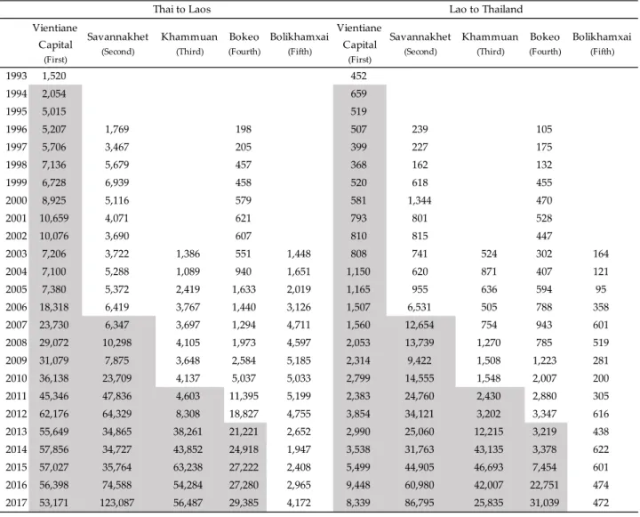
of the bridge, often facilitating less formal trade. Table 1 shows the trade values aggregated by province before and after the completion of the bridge. The gray background indicates the period after the completion of the bridge. The background is white for the fifth bridge, as it is currently under construction. We included this new bridge to highlight the impact of bridges.
=== Table 1 ===
The trade of provinces with bridges has shown a rapid increase. For instance, annual imports by provinces with a bridge for the year 2017 are between 7 and 30 times larger, while annual exports are between 18 and 184 times larger than those without a bridge. Both imports and exports increase after the completion of the bridge, although it takes more time for this to occur in some bridges. Trade in Khammuan (the third bridge) increases the fastest after completion, mainly because it functions as a major transit trade point between Thailand and Vietnam. Savannakhet has the largest values including both exports and imports, perhaps due to the existence of one of the largest copper mines in Laos, in addition to being a major transit trade between Thailand and Vietnam.
According to Keola (2013), international bridges between Laos and Thailand generally increase private imports through cross-border shopping, especially by residents and small- scale traders on Laos’ side, in addition to conventional trade. This is evident from the continued increase in the number of passengers and shuttle buses across these bridges. The main reasons behind this increase are the differences in prices and availability of both agricultural and industrial goods on the Lao and Thai sides. Thailand supplies cheaper agricultural goods based on the scale effect and larger varieties of industrial goods than Laos. Therefore, international bridges between Laos and Thailand generally reduce prices for consumers in Laos through both conventional and cross-border shopping.
3. Empirical Framework
This section discusses our empirical framework to consider the effects of international bridges on households’ living standards. We first introduce the underlying framework for the empirical analysis and then explain the data used in the regression analysis. Finally, we present our empirical model and discuss some of the empirical issues.
3.1. Framework
In the empirical analyses below, we developed a simple framework to interpret the
7
share of food expenditure as an inverse measure of living standards.9 First, we assume two types of goods: food (𝐹𝐹 ) and non-food goods (𝑁𝑁 ). The household budget constraint is expressed as
𝑀𝑀 = 𝑃𝑃𝐹𝐹𝑄𝑄𝐹𝐹+𝑃𝑃𝑁𝑁𝑄𝑄𝑁𝑁, (1)
where 𝑀𝑀 is income or total expenditure. 𝑃𝑃𝐹𝐹 , 𝑃𝑃𝑁𝑁 , 𝑄𝑄𝐹𝐹 , and 𝑄𝑄𝑁𝑁 denote the prices and quantities of food and non-food goods, respectively. The change in the total expenditure becomes
𝑀𝑀̇ =𝑤𝑤𝐹𝐹�𝑃𝑃𝐹𝐹̇ +𝑄𝑄𝐹𝐹̇ �+ (1− 𝑤𝑤𝐹𝐹)�𝑃𝑃𝑁𝑁̇ +𝑄𝑄𝑁𝑁̇ �, (2) where 𝑤𝑤𝐹𝐹 ≡ 𝑃𝑃𝐹𝐹𝑄𝑄𝐹𝐹/𝑀𝑀, and 𝑋𝑋̇ represents the log difference of variable 𝑋𝑋. We further define the change in consumption index or living standards as 𝑄𝑄̇ ≡ 𝑤𝑤𝐹𝐹𝑄𝑄𝐹𝐹̇ + (1− 𝑤𝑤𝐹𝐹)𝑄𝑄𝑁𝑁̇ , and the price index as 𝑃𝑃̇ ≡ 𝑤𝑤𝐹𝐹𝑃𝑃𝐹𝐹̇ + (1− 𝑤𝑤𝐹𝐹)𝑃𝑃𝑁𝑁̇ , so that 𝑀𝑀̇ =𝑃𝑃̇+𝑄𝑄̇ . This equation shows that the change in total expenditure cannot be interpreted as a change in consumption quantity. The precise calculation of the change in the price index is important for measuring changes in living standards.
In standard consumer theory, 𝑄𝑄𝐹𝐹 is determined by the prices of both goods and total expenditure. Therefore, we can derive the following equation by total differentiation:
𝑄𝑄𝐹𝐹̇ = 𝜂𝜂𝐹𝐹𝑀𝑀𝑀𝑀̇+𝜂𝜂𝐹𝐹𝐹𝐹𝑃𝑃𝐹𝐹̇ +𝜂𝜂𝐹𝐹𝑁𝑁𝑃𝑃𝑁𝑁̇ , (3) where 𝜂𝜂𝐹𝐹𝑀𝑀 is the income elasticity of the food demand. This is assumed to be positive but less than one, as in the standard estimation.10 𝜂𝜂𝐹𝐹𝐹𝐹 and 𝜂𝜂𝐹𝐹𝑁𝑁 denote the price elasticities of food demand with respect to food and non-food prices, respectively.
Combining the above equations and the homogeneity of food demand, we can derive the change in the food share as follows:
𝑤𝑤𝐹𝐹̇ = (𝜂𝜂𝐹𝐹𝑀𝑀−1)𝑄𝑄̇+ [(1− 𝜂𝜂𝐹𝐹𝑀𝑀)(1− 𝑤𝑤𝐹𝐹)− 𝜂𝜂𝐹𝐹𝑁𝑁]�𝑃𝑃𝐹𝐹̇ − 𝑃𝑃𝑁𝑁̇ �. (4) This equation shows that the log change in the food share can be interpreted as the change in living standards if the change rate in food price is similar to that in non-food price, 𝑃𝑃̇ = 𝑃𝑃𝐹𝐹̇ = 𝑃𝑃𝑁𝑁̇ . If the construction of the bridge reduces the prices of both goods proportionally, the direct effects of the changes in prices offset each other and disappear in the change rate of the food share. In this study, we assume that the change in the relative food price is not correlated with the distance from the bridge and other variables used in the regression analyses.1112 Using this assumption, we consistently estimate the effects of the bridge on the
9 The framework written in this sub-section is based on Clements and Chen (2010).
10 For example, Seale, Regmi, and Bernstein (2003) estimate the income elasticity of demand for food, beverages, and tobacco as 0.68-0.80 among low-income countries in 1996.
11 International trade theories like the Heckscher-Ohlin model predict that the domestic prices of export goods can increase in response to the reduction of trade costs. Despite this prediction, we consider the changes in both prices as being similar because the main exports of this region are natural resources like copper as described in Section 2, and they are not consumer goods.
12 This assumption justifies the regression of the food share without including the relative food price into a set of explanatory variables. We admit that this method is controversial. Hamilton (2001) demonstrates that omitting the relative food price has small effects on the coefficients for other variables in the model slightly different from this study. Almas, Kjelsrud, and Somanathan (2019) also regress the food share
8
living standards by regressing the change in the food share on the distance from the bridge.
Next, we discuss how the construction of the bridge affected the consumption and living standards of the Lao people. Based on the trade liberalization literature, we consider two channels: changes in income and price. First, the construction of the bridge promoted exports by reducing trade costs, as shown in Table 1, and in turn, increased the wage and income of the people living in this region. While the increase in income would increase the consumption in quantity and value of both food and non-food goods, the food consumption increase is smaller because the income elasticity of food demand is generally small. The other channel shows a drop in prices induced by the reduction in trade costs. While the drop in prices would increase the consumption of food and non-food goods in quantity, the value of food consumption might decrease due to the small price elasticity of food demand. Both channels induce a decrease in the share of food expenditure to total expenditure and improvement in living standards.
Another critical issue to be discussed is the relationship between the impact on trade costs and the distance from the bridge. In this study, we assume that the effects of the bridge were larger for households closer to the bridge, and those households faced a relatively large change in trade costs. The consumer price each household in Laos faced can be considered a combination of export price, river-crossing cost, and domestic transport cost. Even when river-crossing cost dropped sharply, the large domestic transport cost would prevent the consumer prices from falling significantly for households at a distance from the bridge.
Inferring the changes in transport costs and prices is also difficult because many external shocks affected them and the changes depend highly on the locations. In summary, we consider that comparing the change in the food share of the households close to the bridge with the corresponding change of the distant households is one of the best methods for estimating the effects of the bridge on the Laos households.
3.2. Data
In this subsection, we explain the data used in the empirical analysis. Our main source of data is the Lao Expenditure and Consumption Survey (LECS), a household survey conducted by the Department of Statistics. The surveys were conducted over 12-month periods from March to February to control for seasonal variation. The interview month was randomly assigned to each village. Among the six waves of the survey, we employed the third (LECS 3) in 2002/03 (hereafter, 2002) and the fourth survey (LECS 4) in 2007/08 (hereafter, 2007) because these two surveys were conducted before and just after the
without using the relative food price. Gibson, Le, and Kim (2017), in contrast, criticize this food Engel curve method to derive the spatial deflators due largely to the omitted variable bias. We believe the method is valid in our study because we use panel data and all time-invariant factors are controlled for by taking first difference of the food share.
9
construction of the bridge.13 In LECS 4, 518 villages, 8,296 households, and 48,021 individuals were surveyed as 16 households per village were interviewed in almost all villages. Around half of those households were surveyed in the LECS 3.
While the survey covers all regions in Laos, we limit the study sample as some regions in Laos were already connected by another bridge or by land before the construction of the Second Bridge. Specifically, we construct two samples based on the household location. The first sample comprised households located in the bridge province, Savannakhet. Then, as the second sample, we extend the study area by adding households in the two neighboring provinces, Khammuan and Saravane. The sample of the three provinces includes 30 districts, 114 villages, and 920 households.
In this study, we use a consumption-based welfare measure, instead of income, because the change in income cannot capture the change in prices, as discussed in the previous subsection. 14 The consumption-based approach is reflected in the LECS questionnaire, wherein detailed information on household consumption expenditure is collected and recorded. The survey also asked households to keep a diary of their transactions to record their expenses accurately. The consumption captured in the LECS includes both cash expenditures and in-kind expenditure of own-produced goods, except for some durable goods and rents.15 Additional information on purchases of certain high- value goods is collected for the last 12 months, and annual purchase value is divided by 12 to calculate monthly consumption.16
Figure 2 shows the relationship between food share and total expenditure in 2002. As total expenditure increases, the share of food expenditure decreases. This relationship, well- known as Engel’s law, has been studied by many and confirmed both within and between countries. Despite this relationship, we consider the food share as a measure of living standards as we take the change in local prices seriously, and estimating the effects of the bridge on the price changes is difficult. As discussed above, total expenditure change is the summation of the price and quantity indices, and we may misunderstand the effects of the bridge on living standards if we consider the change in the total expenditure without including the precise price index.
=== Figure 2 ===
13 See Department of Statistics (2010) on the detailed procedure for LECS.
14 Bader, Bieri, Wiesmann, and Heinimann (2017) employ the multidimensional poverty approach in Laos.
15 The value of self-consumption is not recorded in the income section of the survey. This is another reason why we prefer the consumption-based measure to the income.
16 While LECS includes the detailed diary, we prefer the use of the food share to the construction of the spatial price index by two reasons. First, the quality of the goods can change both in time series and across regions. Second, transaction costs are not included in the face values of the goods written in the diary. In particular, consumer moving costs must be affected by the construction of the bridge.
10
3.3. Specification
This subsection provides the empirical framework we employ to examine the effects of the Second Bridge’s construction on Laos households. Our estimating equations at the household level are as follows:
Δ𝑌𝑌𝑖𝑖 =𝛼𝛼1𝑇𝑇𝑇𝑇𝑇𝑇𝑇𝑇𝑇𝑇𝑇𝑇𝑇𝑇𝑇𝑇𝑇𝑇𝑑𝑑+𝒙𝒙𝒊𝒊𝜷𝜷𝟏𝟏+𝜀𝜀1𝑖𝑖 (5) Δ𝑌𝑌𝑖𝑖 = 𝛼𝛼2𝐷𝐷𝐷𝐷𝐷𝐷𝑇𝑇𝑇𝑇𝑇𝑇𝐷𝐷𝑇𝑇𝑣𝑣+𝒙𝒙𝒊𝒊𝜷𝜷𝟐𝟐+𝜀𝜀2𝑖𝑖, (6) where 𝑌𝑌𝑖𝑖 indicates the various outcome variables for household 𝐷𝐷 . As explained, our dataset covers 2 years, 2002 and 2007. We take (log) differences in the outcome variables between the 2 years. While our main outcome variable is the food share of household expenditure, we also explore the effects of the bridge on food and non-food expenditures in terms of level and glutinous rice consumption.17 The outcome variables, except for food share, were divided by the number of household members to make the variables use a per capita basis.
Equation (5) shows the model of the DID analysis (hereafter model (A)) to measure the effects of the bridge on Laos households. 𝑇𝑇𝑇𝑇𝑇𝑇𝑇𝑇𝑇𝑇𝑇𝑇𝑇𝑇𝑇𝑇𝑇𝑇𝑑𝑑 is a dummy variable that takes the value of 1 if household location d belongs to the bridge district, Kaysone Phomvihane.
We consider that these households are largely affected by the construction of the bridge. In the robustness checks, we include the neighboring four or five districts along the highway, National Road No. 9 (NR9), in the treatment group. In contrast, the control group comprised households located in other districts in our study sample. As explained above, the whole sample comprised households in Savannakhet or three provinces: Khammuan, Savannakhet, and Saravane.
While the effects of the bridge are expected to be strong for the households near the bridge, we have no specific reasons for limiting the bridge district as the treatment group.
Therefore, we rely on another model (hereafter model (B)), where we use a log of distance to measure exposure for the effects of the bridge.18 The 𝐷𝐷𝐷𝐷𝐷𝐷𝑇𝑇𝑇𝑇𝑇𝑇𝐷𝐷𝑇𝑇𝑣𝑣 in equation (6) is the direct distance of the household location from the bridge measured at the village level, 𝑣𝑣. This analysis assumes that an international bridge has a larger effect on the households closest to the bridge and that the effects fade for households located farther away. As robustness checks, we also estimate the same equations using the road or time distance from the bridge instead of the direct distance.
A vector of 𝒙𝒙𝒊𝒊 indicates household characteristics, which are included as control variables. Specifically, we control for the gender dummy of the household head, the age of
17 In the framework based on AIDS, the dependent variable must be the level change in the food share.
We estimated this case instead of using the log change as the dependent variable, but the estimation results did not change.
18 Notice that the sign of 𝛼𝛼2 is expected be opposite to the sign of 𝛼𝛼1.
11
the household head, the old head dummy that takes a value of 1 if the age of the household head is larger than 60, and the marital status of the head. 𝜀𝜀𝑖𝑖 is a disturbance. In both equations, the households are weighted by population, and standard errors are clustered at the village level. Since the number of observations is not large, we do not restrict the study observations to those wherein all variables were available. The number of study observations differed across the estimations.
There are some endogeneity issues in our empirical framework. Our main concern is omitted variable bias. The location of the bridge was not randomly chosen. If its choice is related to economic conditions, the estimates of our interest variables, 𝛼𝛼1 and 𝛼𝛼2, will be biased. We consider the differences in the economic conditions at the district and household levels. First, if the government chose to construct the bridge in high-growth districts, the error term would be positively correlated with the treatment dummy, yielding an upward bias. Thus, if we obtain positive impacts from the bridge, the magnitude of the results would be overestimated. We deal with this by restricting the sample area and extending the treatment group. Although the population of the villages in Kaysone Phomvihane is the largest among the other districts in the three provinces, no difference in the mean population between the villages along NR9 and the other villages in Savannakhet was found. The initial conditions of the treatment districts are similar to those of the control districts, except for the distance from the bridge, at least in this case.19
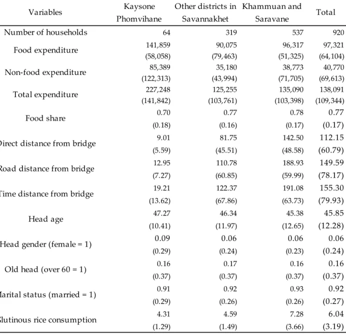
The next point is the difference between households located in the bridge district. If the income of poor households tends to grow faster and the households in the bridge districts are relatively wealthy, the coefficient for the treatment variable would suffer from a downward bias.20 We provide an overview of some statistics for exploring the differences in initial states across households according to their locations. Table 2 compares the outcome and explanatory variables for the year before the establishment of the bridge. We classified the households into three groups by location: Kaysone Phomvihane (the district where the Second Bridge is located), other districts in Savannakhet, and Khammuan and Saravane (neighboring provinces to Savannakhet) and calculated simple averages and standard deviations for each group. The table shows that the households in Kaysone Phomvihane are quite different from those of other districts in Savannakhet and other provinces considering expenditure on food and non-food goods.21 The lower average food share in Kaysone Phomvihane implies that the households in the district were relatively wealthy. This
19 In addition, we confirmed that the estimation results are not largely affected when the log of village population in 2002 is included in the set of explanatory variables.
20 Warr, Rasphone, and Menon (2018) highlight the rise in inequality measured as Gini coefficient in Laos over 1992–2012. In our sample, in contrast, the estimate of the coefficient is -0.67 and statistically significant when we run simple regression of the log difference on the initial level of the food share. This result is not qualitatively changed for each of food and non-food expenditures and when village dummies are included as explanatory variables.
21 Some of the differences of household expenditure can be attributed to the difference of the local prices.
12
difference implies that the improvement in living standards might be attributed to growing inequality caused by other reasons and not by the construction of the bridge, even if the food share is largely reduced for households close to the bridge. In contrast, the table also shows that other variables on household characteristics are not very different between the treatment and control groups. Six percent of our study households had a female head. The average age of the heads was 45.8 years old. On average, households in Kaysone Phomvihane consumed a relatively small amount of glutinous rice in 2002.
=== Table 2 ===
We tackle this identification issue stemming from the large difference in the initial states using two approaches. First, we simply add the initial level of total expenditure in the estimating equations as an explanatory variable. This approach is straightforward, but the obtained results require careful interpretation because the initial total expenditure is an endogenous variable. In the second approach, we also conduct propensity score matching and estimate the average treatment effects for the treated. In this analysis, we first estimate the propensity score of each household to be located in the districts close to the bridge. We use the logit model to estimate the propensity score, and the explanatory variables are household characteristics and initial total expenditure. After estimating the propensity scores, we construct the sample by matching each household in the treatment group with one in the control group, whose propensity score is closest to the treated household. Finally, we compared the differences in outcome variables between the treatment and control groups.
4. Empirical Results
In this section, we report the estimation results. After presenting our baseline results on food and non-food expenditures, we show the robustness of the results using other measurement methods and matching estimates.
4.1. Baseline Results
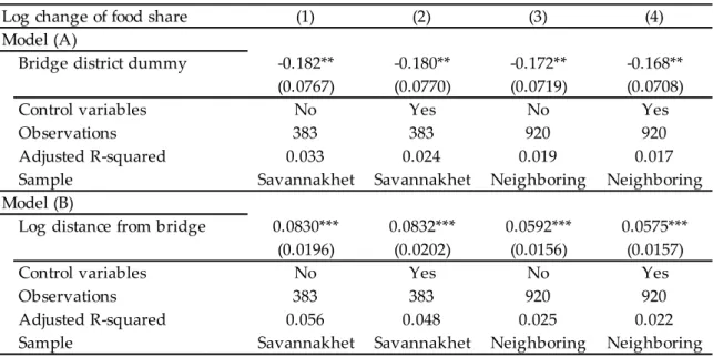
Table 3 shows the estimation results for the share of food expenditures. The upper panel in the table shows the results of model (A), DID analysis using a dummy variable as treatment. The lower panel shows the results of model (B), and the distance from the bridge is the measure of treatment. The first two columns in the table show the estimation results using the Savannakhet sample. In these columns, the coefficients of the treatment dummy and distance are consistent and statistically significant. Both models show that food share
13
largely decreased for households close to the bridge. As shown in the third and fourth columns, the results do not change when including the households in Khammuan and Saravane in the sample. As discussed in the above section, the reduction in food share suggests an improvement in living standards. From the third column in model (B), the household closer to the bridge by 10% is associated with a 0.592% larger food share decrease.
Equation (4) with 𝑃𝑃̇=𝑃𝑃𝐹𝐹̇ =𝑃𝑃𝑁𝑁̇ shows that if the income elasticity of the food demand is 0.75, then the rise in economic welfare, measured by the quantity index, for the household is 2.368(=0.592/(1-0.75))%.
=== Table 3 ===
Next, we highlight each of the expenditures on food and non-food goods. The results are presented in Tables 4 and 5, respectively. We again report the results of model (A) in the upper panels and model (B) in the lower panels. The estimation results in Table 4 show that the food expenditure decreases in households close to the bridge, suggesting that the construction of the bridge decreases the food expenditure. We consider three potential reasons for this negative effect. The straightforward interpretation is that the households around the bridge somehow became poorer, and food consumption decreased in quantity.
We investigate this possibility later and show that this interpretation is not a valid reason.
The second reason is a sharp drop in food prices. In general, the price elasticity of food demand is less than one. Lower prices can induce lower expenditure if the effect of price change dominates the effects of an income increase. Finally, we acknowledge the possibility that the estimates we obtained might be biased due to ignorance of the difference in the initial states of the households. However, Table 5 shows that non-food expenditure increases in households close to the bridge, although almost all the coefficients are statistically insignificant. We also investigate the possibility that the coefficients are biased in the estimations of non-food expenditures.
=== Tables 4 and 5 ===
We found a decrease in food expenditure and highlighted the possibility that the food consumption decrease was a result of the potential negative effects of the bridge on income.
To delve deeper into this point, we estimated the effects of the bridge on glutinous rice consumption. The consumption of glutinous rice would be negatively affected by the construction of the bridge if the food consumption of households close to the bridge decreased in quantity. Table 6 presents the estimation results. While the estimates of the coefficients are not stable and most of them are statistically insignificant, we can say that the rice consumption of households close to the bridge does not clearly decrease. The results are not consistent with the interpretation that the households around the bridge somehow
14
became poorer, and food consumption fell in quantity after constructing the bridge. Among the three reasons for the food expenditure decrease, we consider that in the second and the third, the dominant effects of a drop in the food price and the omitted variable bias are more convincing.
=== Table 6 ===
4.2. Robustness Checks
In this subsection, we check the robustness of the results. We first employed other measures for the treatment dummy. We included four neighboring or five districts along NR9 in the treatment group. If the previous estimation results were attributed to the prosperity of Kaysone Phomvihane, the significant effects on the food share would disappear when we included other districts in the treatment group. Table 6 shows the estimation results using alternative treatment dummy variables. The coefficients on the food share are all negative and statistically significant, even if the treatment dummy takes 1 for households in the districts neighboring Kaysone Phomvihane or along NR9.22 However, the coefficients for food expenditures are vulnerable and become statistically insignificant if the treatment group is expanded to neighboring districts or districts along the NR9.
=== Table 7 ===
We then check the robustness of the results when we employ alternative definitions of distance measures. In addition to the direct distance in the baseline results, we use the road and time distances because people moving by car drove on the road, and time was one of the most important factors in the trade costs. Table 8 presents the estimation results using alternative measures of distance. The coefficients for the food share are all positive and statistically significant. The food share robustly decreased in households close to the bridge.
Unlike the estimation results shown in Table 7, the coefficients for food expenditure in Table 8 do not change and are statistically significant only if the sample is limited to Savannakhet.
The results on the log change in the non-food expenditures weakly suggest that the construction of the bridge increases the non-food expenditures.
=== Table 8 ===
22 Riano and Caicedo (2020) found persistent negative impacts of bombing in Laos, using the relationship between the number of bombs dropped and distance to the Vietnam border. Our results on alternative measurements reject the possibility that our baseline results are obtained from the effect of bombing and unexploded ordnance on the change in the food share as NR9 extends from the Second Bridge to the Vietnam border.
15
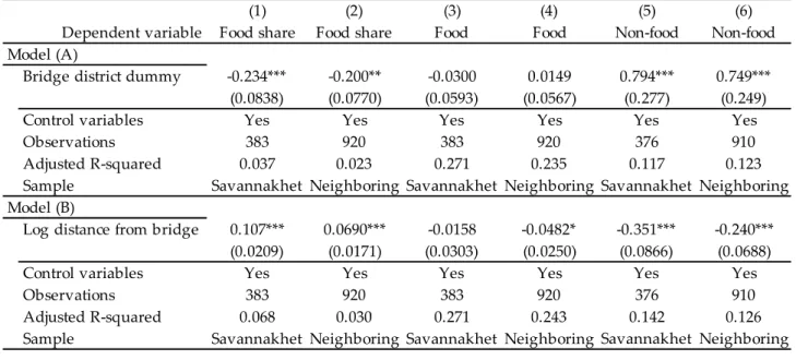
We then investigate how the difference in initial states among households affects the estimation results in the above DID analysis. To address this problem, we first added control variables to the baseline analyses. In this estimation, the initial level of total expenditure is included as an explanatory variable. The results are listed in Table 9. The coefficients for food share in the first two columns are negative and statistically significant. The food share decrease was not affected by the initial levels. In contrast, the results in the third and fourth columns show that the bridge has almost no effect on the food expenditures, suggesting that the coefficients in the DID analysis above might be biased because of the difference in the initial states. Additionally, we can clearly see large and statistically significant coefficients on the log change in the non-food expenditures when the initial total expenditure is controlled for. While cautious interpretation is required for these results in this table as the total expenditure is an endogenous variable, the estimation results suggest that non-food goods expenditures largely increased in households close to the bridge.
=== Table 9 ===
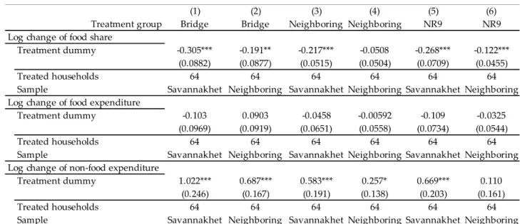
To confirm the results of the previous analysis, we compare households with similar characteristics. Table 10 presents the estimation results of propensity score matching. In the upper panel, the coefficients on food share are negative and statistically significant, except for the fourth column. The middle panel shows the estimation results for the log change in food expenditure; however, all coefficients are insignificant. In contrast, in the lower panel, the coefficients for non-food expenditures are positive and statistically significant. We report the standardized differences in the variables in Table 11 to check the balance of the covariates. As shown in Table 2, we can see a large difference in initial total expenditure between households in the treatment and control groups for the whole sample. However, the difference in the initial total expenditure decreased for the matched samples. One of the standard criteria for standardized differences is 0.1. While some of the variables are over the criterion, we consider that the control group is appropriately chosen as a whole.
=== Tables 10 and 11 ===
In this subsection, we checked the robustness of the estimation results. Most of the results are robust to alternative measures for the treatment group and the distance from the bridge. While the effects of the bridge on the food and non-food expenditures estimated in the DID analysis may be biased due to ignorance of the difference in the households’ initial states, the effect on the food share is robust. Ultimately, these results strongly suggest that the construction of the bridge improved the living standards of households close to the bridge. Although the effects on the change in food expenditures are ambiguous due to the offsetting price change, the non-food expenditures increased after the construction of the
16
bridge.
5. Heterogeneous Treatment Effects
In this section, we explore the heterogeneity of the treatment effect on Laos households.
The impacts of trade policy on households have been shown to be heterogeneous in several studies. For example, Porto (2006) found that Mercado Común del Sur or Sothern Common Market (Mercosur) benefited poorer more than richer families in Argentina. Han, Liu, Ural Marchand, and Zhang (2016) also found heterogeneous effects of China’s WTO accession to be pro-poor. However, not all trade policies benefit the poor more. For example, Nicita (2009) investigates trade liberalization in Mexico in 1990–2000 using price and wage data and concludes that although tariff liberalization has had a net positive impact on households, the purchasing power of households with income largely depending on agricultural activities or unskilled wages decrease. Here, richer or more skilled households are found to benefit more from trade policy.
This section investigates whether the second friendship bridge has heterogeneous effects on households in the three provinces of Laos. However, applying the methodologies in the literature on trade liberalization is difficult, as we focus on a much smaller area, that is, a particular international bridge, and households that are distributed within only about 300 km from it. This reduces the number of observations substantially, making it very difficult to establish a statistically significant relationship within each interested household group. These issues motivate the study of the heterogeneous effects by machine learning approaches.
5.1 What is a Causal Forest?
In this study, we turn to an emerging machine learning technique whose major benefit is its ability to fit linear and nonlinear relationships even with a small number of observations. We specifically make use of the causal tree proposed by Athey and Imbens (2017). The causal forest applies a machine learning method called a decision tree. A decision tree is a statistical learning method that reproduces nonlinear relationships by recursively creating branches from independent to dependent variables. For a demonstration purpose, Figure 3a illustrates a decision tree predicting the share of food expenditure for the first 50 households in our observations with the age of household head and total expenditure. We limit the number of samples to 50, and the minimum is split to 10 to simplify the tree for display and reading on the screen. The minimum split is the threshold of the minimum number of data points in a leaf to stop splitting. Figure 3b compares the prediction by this single tree in Figure 3a with real data. The precision of
17
prediction can be observed by how many predicted vs. real data points overlap. Decreasing the minimum tree split increased the prediction precision (Figure 3c). Note that a complete prediction, wherein all predictions lie above real data points, is always possible by limiting the number of covariates and minimizing it to 1.
A major drawback of a partition tree is overfitting, which means that it is unable to predict an out-of-sample relationship. Causal forests cope with this problem by randomly splitting data into one for prediction and the rest for evaluation and grow many (e.g., 2000) trees fine-tuned using the prediction of evaluation data. Basically, instead of growing one tree that would easily overfit the original data, a causal tree attains “honesty” by randomly choosing different subsets for growing trees (forest), while using the rest for testing how good they predict evaluation data. Subsequent studies have used this package to study heterogeneous treatment effects (among others, Davis and Heller, 2017; Fuster et al., 2020).
=== Figure 3 ===
5.2 Heterogeneous Treatment Effects Predicted by Causal Forest
Here, we apply the causal forest to model (A) specified in Section 3.3. Covariates include age, gender, marital status of the household head, and total expenditure in 2002.
Treatment is either in the district where the bridge was built (Kaysone Phomvihane) or in districts connected to the bridge with the quality road (NR9). Control groups are divided into the provinces with bridges (Savannakhet) or that extends to two adjacent provinces (Savannakhet, Khammuan, and Saravane). Note that the treatment effects are also predicted for households that are not actually treated. Basically, this is what would have happened for individual households if they were in the district with the bridge or districts connected to the bridge with a good-quality road.
First, we show the treatment effects predicted by the causal forest on a map (Figure 4).
We start by focusing on the case wherein the district with the bridge is considered the treatment (Figure 4, columns 1 and 3). Causal forests predict all households to reduce their food share expenditure (Figure 4, row 1, columns 1 and 3). While the scales of treatment effect predicted by causal forest are not exactly the same because the sizes of negative signs are different, almost all households could benefit from the bridge. Similarly, a causal forest predicts that all households will increase non-food expenditure (row 3, columns 1 and 3).
These two findings fit the DID analysis (Tables 3 and 5) in the previous section. In contrast, the causal forest predicts both positive and negative effects on food expenditure (Figure 4, row 2), and when districts connected to the bridge are considered the treatment (Figure 4, columns 2 and 4). Causal forests predict an even more heterogeneous treatment effect when connectivity to the bridge via a good-quality road is considered the treatment.
18
=== Figure 4 ===
We can further investigate the heterogeneity of treatment effects using scatter plots of individual households (Figure 5). Here, we focus on the variation to determine if the scale of heterogeneity is large. In general, the variation is smaller when the district with the bridge is considered the treatment (Figure 5, columns 1 and 3), compared to the case when districts along NR9 are considered the treatment (Figure 5, columns 2 and 4). Basically, the causal forest predicts households to benefit from the bridge in the same way if they were in the district where the bridge was constructed. In contrast, households are predicted to benefit (or not benefit) quite differently if they are in districts with a long NR9. Therefore, this section’s last task is to investigate the causes of this large heterogeneity with indirect access via NR9.
=== Figure 5 ===
Figure 6 illustrates the treatment effect predicted by the causal forest by the order of the total expenditure in 2002. We do not report the same figures with other covariates related to the household head’s characteristics as we find no particular patterns in them. We first focus on the case when heterogeneous treatment effects are relatively large, that is, when connectivity to the bridge with the quality road is considered the treatment (Figure 6, columns 2 and 4). All treatment effects seem to follow an obvious trend when plotted against the average total expenditure in 2002 if NR9 was considered the treatment. For example, households with higher total expenditure (i.e., richer households) are predicted to reduce their food share more than poor households (Figure 6, row 1, columns 2 and 4). Richer households also tended to increase food expenditure more (Figure 6, row 2, columns 2 and 4). The same holds for non-food expenditure (Figure 6, row 3, columns 2 and 4). Although the total expenditure also affects the predicted treatment effects when the district with the bridge is considered the treatment, the effects do not seem to follow certain obvious patterns (Figure 6, columns 1 and 3). In brief, causal forests predict heterogeneous treatment effects.
The variation in treatment effects is relatively small and does not follow any obvious trend if the households were in (moved to) the district with the bridge. Richer households would benefit more from the bridge if they were in (moved to) districts along NR9, although the poorer could also benefit from the bridge in this case.
=== Figure 6 ===
6. Concluding Remarks
19
This study investigates the impact of an international bridge constructed between Thailand and Laos on Laos households. Using the household survey, we conducted the DID to explore the change in the share of food expenditure to total expenditure. Our estimation results show that establishing an international bridge decreased the food share, suggesting that the living standards of households close to the bridge were improved. Our results on food share are robust when we consider the large initial difference between the treatment and control groups. We also found that income level, captured by the total expenditure, is responsible for the heterogeneity of the treatment effects; however, it is not large across households when direct access to the bridge is considered the treatment. The heterogeneity of the treatment effects becomes larger when indirect access to the bridge through the quality road is considered the treatment.
We acknowledge some limitations of the analyses. First, our major indicator, food share, is not a direct measure of living standards. While the use of the food share fits our purpose and our dataset, measurement errors and biases are not completely excluded.
While we attempted the back-to-the-envelope calculation for the effects of the bridge, the use of indirect measures also makes it difficult to precisely quantify the welfare effects of the international bridge. A comparison of costs and benefits is important for evaluating the construction of infrastructure. Additionally, while we confirm the robustness by alternative definitions of treatment and the analyses using the distance measures, we do not have compelling reasons to consider the bridge district as the treatment group and others as controls. Finally, we cannot reject the possibility that some confounding factors may have influenced the results obtained in the analyses. While we estimate the treatment effects using the propensity score matching method, the method also depends on some strong assumptions.
Regardless of the limitations, we believe our analyses are helpful in clarifying the roles of the transport infrastructure in developing countries’ development strategies.
Constructing the international bridge has positive effects on the living standards of households in developing countries. Our results are also important when considering the possibility that developing high-quality domestic transport infrastructure complements the construction of the international transport infrastructure. In the case of Laos, paved roads may play a vital role in enhancing the usefulness of the international bridge and promoting international trade and price integration with other countries. These infrastructures would be more fruitful for rural areas and help reduce inequality across regions.
20
References
Akerman, A., 2009, Trade, Reallocations and Productivity: A Bridge between Theory and Data in Oresund, Mimeograph, Stockholm University.
Almås, I., 2012, International Income Inequality: Measuring PPP bias by estimating Engel curves for food. American Economic Review, 102(2): 1093–1117.
Almås, I., Kjelsrud, A., and Somanathan, R., 2019, A Behavior-Based Approach to the Estimation of Poverty in India. Scandinavian Journal of Economics, 121(1): 182–224.
Andersson, M., Engvall, A., and Kokko, A., 2007, Regional development in Lao PDR:
growth patterns and market integration, Mimeograph, Stockholm School of Economics.
Armenter, R., Koren, M., and Nagy D. K., 2014, Bridges, Mimeograph, Central European University.
Athey, S., 2017, Beyond prediction: Using big data for policy problems, Science, 355(6324):
483-485.
Athey, S., and Imbens, G. W., 2017, The state of applied econometrics: Causality and policy evaluation. Journal of Economic Perspectives, 31(2): 3–32.
Bader, C., Bieri, S., Wiesmann, U., and Heinimann, A., 2017, Is economic growth increasing disparities? A multidimensional analysis of poverty in the Lao PDR between 2003 and 2013. Journal of Development Studies, 53(12): 2067–2085.
Banks, J., Blundell, R., and Lewbel, A., 1997, Quadratic Engel curves and consumer demand. Review of Economics and Statistics, 79(4): 527–539.
Björkegren, D., and Grissen, D., 2020, Behavior revealed in mobile phone usage predicts credit repayment. World Bank Economic Review, 34(3): 618–634.
Brooks, W., and Donovan, K., 2020, Eliminating uncertainty in market access: The impact of new bridges in rural Nicaragua. Econometrica, 88(5): 1965–1997.
Clements, K. W., and Chen, D., 2010, Affluence and food: a simple way to infer incomes.
American Journal of Agricultural Economics, 92(4): 909–926.
Coondoo, D., Majumder, A., and Chattopadhyay, S., 2011, Estimating spatial consumer price indices through Engel curve analysis. Review of Income and Wealth, 57(1): 138–155.
Costa, D. L., 2001, Estimating real income in the United States from 1888 to 1994: Correcting CPI bias using Engel curves. Journal of Political Economy, 109(6): 1288–1310.
Dai, M., Huang, W., and Zhang, Y., 2020, Persistent effects of initial labor market conditions:
The case of China’s tariff liberalization after WTO accession. Journal of Economic Behavior and Organization, 178: 566–581.
Dai, M., Huang, W., and Zhang, Y., 2021, How Do Households Adjust to Tariff Liberalization? Evidence from China’s WTO Accession, forthcoming in Journal of Development Economics.
21
Davis, J., and Heller, S. B., 2017, Using causal forests to predict treatment heterogeneity:
An application to summer jobs.” American Economic Review 107(5): 546–50.
De Carvalho Filho, I., and Chamon, M., 2012, The myth of post-reform income stagnation:
Evidence from Brazil and Mexico. Journal of Development Economics, 97(2): 368–386.
Deaton, A., and Muellbauer, J., 1980, An almost ideal demand system. American Economic Review, 70(3): 312–326.
Department of Statistics, 2010, Poverty in Lao PDR 1992/3-2007/8, Vientiane: Department of Statistics.
Fuster, A., Goldsmith-Pinkham, P., Ramadorai, T., and Walther, A., 2020, Predictably unequal? The effects of machine learning on credit markets. Mimeograph.
Gibson, J., Le, T., and Kim, B., 2017, Prices, Engel curves, and time-space deflation: Impacts on poverty and inequality in Vietnam. World Bank Economic Review, 31(2): 504–530.
Gibson, J., Stillman, S., and Le, T., 2008, CPI bias and real living standards in Russia during the transition. Journal of Development Economics, 87(1): 140–160.
Glaeser, E. L., Hillis, A., Kominers, S. D., and Luca, M., 2016, Crowdsourcing city government: Using tournaments to improve inspection accuracy, American Economic Review, 106(5), 114–118.
Han, J., Liu, R., Ural Marchand, B., and Zhang, J., 2016, Market structure, imperfect tariff pass-through, and household welfare in urban China, Journal of International Economics, 100: 220–232.
Hayakawa, K., Keola, S., Sudsawasd, S., and Yamanouchi, K., 2020, The impact of an international bridge on households: evidence from household panel data in Thailand, IDE Discussion Paper No. 794, Chiba: IDE-JETRO.
Inthakesone, B., and Kim, T., 2016, Impact of public road investment on poverty alleviation in rural Laos. International Journal of Applied Business and Economic Research, 14(10):
6339–6350.
Keola, S., 2013, Impacts of Cross-Border Infrastructure Developments: The Case of the First and Second Lao—Thai Mekong Friendship Bridges, In Ishida, M. (ed.), Border Economies in the Greater Mekong Subregion, London: Palgrave Macmillan, 163–185.
Kleinberg, J., Ludwig, J., Mullainathan, S., and Obermeyer, Z., 2015, Prediction policy problems, American Economic Review, 105(5), 491–495.
Nicita, A., 2009, The price effect of tariff liberalization: Measuring the impact on household welfare, Journal of Development Economics, 89(1): 19–27.
Oraboune, S., 2008, Infrastructure Development in Lao PDR, in Kumar, N. (ed.), International Infrastructure Development in East Asia – Towards Balanced Regional Development and Integration, ERIA Research Project Report 2007-2, Chiba: IDE-JETRO, 166–203.
Porto, G. G., 2006, Using survey data to assess the distributional effects of trade policy, Journal of International Economics, 70(1): 140–160.
22
Redding, S. J., and Turner, M. A., 2015, Transportation costs and the spatial organization of economic activity. Handbook of Regional and Urban Economics, 5: 1339–1398.
Riaño, J. F., and Valencia Caicedo, F., 2020, Collateral Damage: The Legacy of the Secret War in Laos. Mimeograph.
Seale Jr, J., Regmi, A., and Bernstein, J., 2003, International Evidence on Food Consumption Patterns, United States Department of Agriculture, Economic Research Service.
Ural Marchand, B., 2012, Tariff pass-through and the distributional effects of trade liberalization, Journal of Development Economics, 99(2): 265–281.
Volpe Martincus, C., Carballo, J., Garcia, P., and Graziano, A., 2014, How Do Transport Costs Affect Firms’ Exports? Evidence from a Vanishing Bridge, Economics Letters, 123:
149–153.
Wager, S., and Athey, S., 2018, Estimation and inference of heterogeneous treatment effects using random forests, Journal of the American Statistical Association, 113(523): 1228–1242.
Warr, P., 2010, Roads and poverty in rural Laos: An econometric analysis. Pacific Economic Review, 15(1): 152–169.
Warr, P., Rasphone, S., and Menon, J., 2018, Two decades of declining poverty but rising inequality in Laos. Asian Economic Journal, 32(2): 165–185.
23
Table 1. Provincial trade with and without bridges
Source: Bank of Thailand.
Notes: The gray background signifies the period after completion of the bridge in the respective provinces.
The unit of the number is million Thai Baht.
24
Table 2. Summary statistics in 2002
Source: Authors’ calculation, using Lao Expenditure and Consumption Survey.
Notes: The number of observations differs slightly by variable. Simple means and standard deviations (in parentheses) are reported. Expenditures were measured using a kip. Direct and road distances were measured in kilometers. The time distance was measured in minutes. The units of glutinous rice consumption were the number of balls per day.