Numerical Existence Proofs and Guaranteed Error Bounds for Solutions to Two-Point Boundary Value Problems (Recent Developments of Numerical Analysis and Numerical Computation Algorithms)

(1)

Numerical Existence Proofs

and

Guaranteed Error Bounds for

Solutions to Two-Point

Boundary Value

Problems

早稲田大学基幹理工学研究科高安亮紀 (Akitoshi Takayasu)1

Graduate School of Fundamental Science and Engineering,

Waseda University

早稲田大学大石進一 (Shin‘ichi Oishi)2

筑波大学久保隆徹 (Takayuki Kubo)3

Abstract –In this article,

a

numerical method ispresented forverifying theexistence

and the uniquenessofsolutions to two-point boundary value problems of second order

ordinary differential equations. By solving the bilinear form of the problem,

a

weak

solution is

a zero

point of

a

certain nonlinear map. The Fr\’echet differentiability of

this nonlinear map isshown. Based

on

the Newton-Kantorovich theorem,

a

numerical

existence and local uniqueness theorem is presented for a zero point of the nonlinear

map. It is shown that taking into account all

errors

of numerical computations such

as discretization errors and rounding errors, conditions of this theorem canbe checked

by numerical computations with result verification. Finally, an illustrative numerical

result is presented for showing the usefulness ofthe method.

1 Introduction

Let $(0,1)$ be

an

open interval. This article is concerned with the two boundary value problem

of the second order ordinary differential equation:

$\{\begin{array}{ll}-(pu’)’=f(u) 0<x<1,u(0)=u(1)=0, \end{array}$ (1)

where $p(x)$ is a smooth function on $(0,1)$ with$p(x)\geq p_{0}>0$ for some $p_{0}$

.

Here, $f$ : $H_{0}^{1}(0,1)arrow$

$L^{2}(0,1)$ is assumed to beFr\’echet differentiable. For example, the following function

$f(u)=-qu’-c_{1}u+c_{2}u^{2}+c_{3}u^{3}+\ldots+c_{N}u^{N}+g$

with $N\in \mathbb{N},$ $q(x),$$c_{i}(x)\in L^{\infty}(O, 1),$ $(i=1, \ldots, N)$ and $g(x)\in L^{2}(0,1)$ satisfies this condition. We

shall propose anumericalverification method for proving the existence of solutions to problem (1).

Studies on this type of computer assisted proofs for the existence of solutions to two point

boundary value problems have been started by pioneering works of Kantorovich [1] and Urabe [2].

Theworks of McCarthy and Tapia [3] andof Kedem [4] $hav\overline{e}$followed. In 1988, M. T. Nakao [5] has

presented

a

method of

a

computer assisted prooffor the existence of solutions to elliptic problems

including the problem (1). This method has shown to be quite useful to generate tight numerical

inclusion of solutions [6]. Nakao’s method can be considered as an interval extension of the finite

element method based on some fixed-point theorem. In 1991, Plum [7] has also presented another

ltakitoshiOsuou.waseda.jp

2Departmentof Applied Mathematics, Faculty ofScienceand Engineering, Waseda University&CREST, JST

(2)

method of proving the existence and uniqueness of solutions for the problem (1). In his method,

the norm of the inverse of linearlized operator is bounded by an eigenvalue enclosing technique

based

on

the homotopy method. Inthese two decades, both Nakao’s method and Plum’s method

have been demonstrated to be quite usefulfor the computer assisted existence proof of solutions of

variousboundary valueproblems of differential equations.

This article presents another method of a computer assisted proofprocedure for the existence

of solutions to the problem (1). In the verification theory, a weak formulation is led from the

original problem. A weak solution is defined

as

a zero

point of

a

certain nonlinear map from

$H_{0}^{1}(0,1)$ into $H^{-1}(0,1)$ in this formulation. Then the Fr\’echet differentiability of this nonlinear

map is shown. Based on the Newton-Kantorovich theorem [1], a numerical existence and local

uniqueness theorem is derived for a zero point of this nonlinear map. This method is based on

the theorem of estimating operator norm of inverse. This theorem makes it possible to obtain

a

numerical existence and local uniqueness theorem. It is also shown that taking into account all

errors

of numerical computations such

as

discretization

errors

and rounding errors, conditions of

this theorem applied to this nonlinear map

can

be checked by numerical computations with result

verification. One offeatures inthis method is that verification conditions

can

be derivedby

a

pure

analytic way.

2 Verification Theory

Inthis section,

we

shallpresent

a

numerical method for verifyingthe existence and the

unique-ness

of solutions to two-point boundary value problems of the second order ordinary differential

equation (1).

2.1 Preliminary

Throughoutthis article, let $L^{2}(0,1)$ denotethefunctional space of Lebesgue-measurable

square-integrable functions with $L^{2}$-inner product and $L^{2}$

-norm

$(u, v)= \int_{0}^{1}u(x)v(x)dx$ and $\Vert u\Vert_{L^{2}}=\sqrt{(u,u)}$, $(u, v\in L^{2}(0,1))$,

respectively. Let $H^{m}(0,1)$ denote $L^{2}$-Sobolev space oforder _$m$ with the inner product

$\langle u,$$v\rangle_{m}=(u, v)+(u’, u’)+\cdots+(u^{(m)}, u^{(m)})$

and the norm [8]

$\Vert u\Vert_{H^{m=\sqrt{\langle uu\rangle_{m}}=}}\sqrt{\Vert u\Vert_{L^{2}}^{2}+\Vert u’\Vert_{L^{2}}^{2}++\Vert u^{(m)}\Vert_{L^{2}}^{2}}$

.

Here, both ’ _and $\frac{d}{dx}$ denote the differentiation with respect to $x$ and $u^{(m)}$ is the m-th derivativeof

$u$ with respect to $x$

.

Let further

$H_{0}^{1}(0,1)=\{u\in H^{1}:u(O)=u(1)=0\}$

with theinner product $(u’, v’)$ and the norm $\Vert u\Vert_{H_{0}^{1}}=\Vert u’\Vert_{L^{2}}$. Let $H^{-1}(0,1)$ bethe topological dual

space of $H_{0}^{1}(0,1),$ $i.e$

.

the space of linear continuous functionals on $H_{0}^{1}(0,1)$

.

Let $T\in H^{-1}(0,1)$

and $u\in H_{0}^{1}(0,1)$

.

We denote$Tu\in \mathbb{R}$ as $<T,$$u>$

.

The norm of$T\in H^{-1}(0,1)$ is defined as

(3)

Let $L^{\infty}(O, 1)$ denote the space of functions that are essentially bounded on _$[0,1]$ with the norm

$\Vert u\Vert_{\infty}=ess\sup_{0\leq x\leq 1}|u(x)|$

.

Let $X$ and $Y$ be Banach spaces. The set of bounded linear operators is denoted by _{$\mathcal{L}(X, Y)$} _with

the operator norm

$\Vert \mathcal{T}\Vert_{\mathcal{L}(X,Y)}=\sup_{u\in X\backslash \{0\}}\frac{\Vert \mathcal{T}u\Vert_{Y}}{||u\Vert_{X}}$, $(\mathcal{T}\in \mathcal{L}(X, Y))$

.

Here, $\Vert\cdot\Vert_{X}$ is the

norm

of$X$ and $\Vert\cdot\Vert_{Y}$ is the

norm

of$Y$

.

The Sobolev embedding theorem states

[6, 8] that

(1) for $(k>l)$ _the_embedding $H^{k}(0,1)arrow H^{l}(0,1)$ is compact and continuous,

(2) the embedding $H_{0}^{1}(0,1)arrow C^{0}(0,1)$ is compact and continuous,

(3) and $H_{0}^{1}(0,1)\subset L^{p}(0,1)$ for_{$p\geq 2$} with

$\Vert v\Vert_{Lp}\leq C_{e,p}\Vert v\Vert_{H_{0}^{1}}$, $(v\in H_{0}^{1}(0,1)$ ex. $C_{e,p}=( \frac{2}{p+2})^{\frac{1}{p}})$

.

(2)

2.2 Weak Formulation and its Fr\’echet _{Differentiability}

Let

us

be concerned with the two-point boundaryvalue problem ofthe form

$\{\begin{array}{ll}-(pu’)’=f(u) 0<x<1,u(0)=u(1)=0. \end{array}$ (3)

In this part,

we

shall present

a

numerical _{verification method of proving the existence of weak}

solutions for Eq. (3). For $u,$$v\in H_{0}^{1}(0,1)$ let us define a continuous bilinear form $a(u, v)$

as

$a(u, v)=(pu’, v’)$

.

If we fix $u\in H_{0}^{1}(0,1)$, then $a(u, \cdot)\in H^{-1}(0,1)$

.

Thus, we can define an _operator $\mathcal{A}$ : _{$H_{0}^{1}(0,1)arrow$}

$H^{-1}(0,1)$ by

$<\mathcal{A}u,$$v>=a(u, v)$,

which

can

be

seen as a

weak form of thedifferentialoperator- $\tau_{x}d(p_{Tx}d)$

.

It is noted that thebilinear

form $a$ is coercive, i.e., $a(u, u)\geq p_{0}\Vert u\Vert_{H_{0}^{1}}^{2}$

.

Then, for $v\in H_{0}^{1}(0,1)$ Lax-Milgram’s theorem states

theexistence of

a

unique solution for the following equation:

$a(u, v)=<T,$$v>$, $(T\in H^{-1}(0,1))$

.

₍₄₎

Ifwe denote the operator which maps $T$ to the solution $u$ of Eq. (4) by $\mathcal{K}$ : _{$H^{-1}(0,1)arrow H_{0}^{1}(0,1)$},

then this theorem also declares that $\mathcal{K}$ becomes an isomorphism between _{$H^{-1}(0,1)$}

and $H_{0}^{1}(0,1)$

.

It is easy to see that

$A\mathcal{K}=\mathcal{I}_{H^{-1}}$ and

$\mathcal{K}\mathcal{A}=\mathcal{I}_{H_{0}^{1}}$

.

Here, $\mathcal{I}_{H^{-1}}$ and $\mathcal{I}_{H^{1}}$ are identity operators on $H^{-1}(0,1)$ and _{$H_{0}^{1}(0,1)$}, respectively. In

the rest

of this article, we $d_{enote}$ _{the identity operator by}

$\mathcal{I}$ omitting the subscript. Thus, we see $\mathcal{K}$ :

$H^{-1}(0,1)arrow H_{0}^{1}(0,1)$ is theinverse of$\mathcal{A}$ : _{$H_{0}^{1}(0,1)arrow H^{-1}(0,1),$} _$i.e$

.

$\mathcal{K}=\mathcal{A}^{-1}$

.

Similarly, for $u,$$v\in H_{0}^{1}(0,1)$

we can

define an operator$\mathcal{N}:H_{0}^{1}(0,1)arrow H^{-1}(0,1)$ by

(4)

Then, a weak form ofEq. (3) canbe written as

$\mathcal{A}u=\mathcal{N}u$

.

(5)

In the following, we will discuss how to verify the existence and the uniqueness of the solution

ofEq. (5), the weak solution of the problem (3). Here,

we

notethat the bilinear form $a(u, v)$ is

an

inner product on $H_{0}^{1}(0,1)$ and there exist positive constants $C_{a}$ and $c_{a}$ satisfying

$c_{a}\Vert u\Vert_{H_{0}^{1}}\leq\Vert u\Vert_{a}\leq C_{a}\Vert u\Vert_{H_{0}^{1}}$ for $u\in H_{0}^{1}(0,1)$, (6)

where $\Vert u\Vert_{a}=\sqrt{a(u,u)}$

.

In fact, we can choose _{$c_{a}=\sqrt{p_{0}}$} and $C_{a}=\sqrt{\Vert p\Vert_{L}\infty}$

.

We define the

operator $\mathcal{F}:H_{0}^{1}(0,1)arrow H^{-1}(0,1)$ by$\mathcal{F}u=(\mathcal{A}-\mathcal{N})u$

.

Then, Eq.(5) can be written as

$\mathcal{F}u=0$

.

(7)

Definitely, the weak solution of (3) is defined as a zero point ofthisnonlinear map $\mathcal{F}$

.

Next, we now show that $\mathcal{F}$ : $H_{0}^{1}(0,1)arrow H^{-1}(0,1)$ is Fr\’echet differentiable. For a fixed _{$u,\hat{u}\in$}

$H_{0}^{1}(0,1)$ we can define $N’(\hat{u})(u, v)$ for $v\in H_{0}^{1}(0,1)$. It is clear that $N’(\hat{u})(u, \cdot)\in H^{-1}(0,1)$

.

Thus,

we candefine anoperator $\mathcal{N}’(\hat{u})$ : $H_{0}^{1}(0,1)arrow H^{-1}(0,1)$ by

$<\mathcal{N}’(\hat{u})u,$_{$v>=N’(\hat{u})(u, v)=(f’(\hat{u})u, v)$}

.

Here, $f’(\hat{u})$ : $H_{0}^{1}(0,1)arrow L^{2}(0,1)$ is the Fr\’echet derivative of $f$ : $H_{0}^{1}(0,1)arrow L^{2}(0,1)$ at $\hat{u}$

.

We

now show that for a given $u\in H_{0}^{1}(0,1)$ the \ddagger he’chet derivative $\mathcal{F}’(u)$ : $H_{0}^{1}(0,1)arrow H^{-1}(0,1)$ of

$\mathcal{F}:H_{0}^{1}(0,1)arrow H^{-1}(0,1)$ is given as

$\mathcal{F}’(u)v=(\mathcal{A}-\mathcal{N}’(u))v$

.

In fact, for $u,$$v\in H_{0}^{1}(0,1)$, we have

$|<\mathcal{N}(u+v)-\mathcal{N}u-\mathcal{N}’(u)v,$ _$w>|$

$\Vert \mathcal{F}(u+v)-\mathcal{F}(u)-(\mathcal{A}-\mathcal{N}’(u))v\Vert_{H^{-1}}=$ _$\sup$

$w\in H_{0}^{1}(0,1)\backslash \{0\}$ $\Vert w\Vert_{H_{0}^{1}}$

$|(f(u+v)-f(u)-f’(u)v, w)|$

$= \sup_{w\in H_{0}^{1}(0,1)\backslash \{0\}}$ $\Vert w\Vert_{H_{0}^{1}}$

$\leq\Vert\mu(u, v)\Vert_{L^{2}}$

.

Here, $\mu(u, v)=f(u+v)-f(u)-f’(u)v$

.

From theFr\’echetdifferentiabilityof$f$ : $H_{0}^{1}(0,1)arrow L^{2}(0,1)$,

we have

$\frac{\Vert\mu(u,v)\Vert_{L^{2}}}{\Vert v\Vert_{H_{0}^{1}}}arrow 0$, $(\Vert v\Vert_{H_{0}^{1}}arrow 0)$

.

This shows the Fr\’echet differentiability of$\mathcal{F}$ : $H_{0}^{1}(0,1)arrow H^{-1}(0,1)$ at $u\in H_{0}^{1}(0,1)$ and

$\mathcal{F}’(u)=\mathcal{A}-\mathcal{N}’(u)$

.

Now, we define the naturalembedding operator $i_{L^{2}rightarrow H^{-1}}$ : $L^{2}(0,1)arrow H^{-1}(0,1)$ by

$i_{L^{2}-H^{-1}}w=T_{w}$, $T_{w}(v)=(w, v)$ for $v\in H_{0}^{1}(0,1)$.

Since$i_{L^{2}arrow H^{-1}}$ : $L^{2}(0,1)arrow H^{-1}(0,1)$ is compact and $f’(\hat{u})$ : $H_{0}^{1}(0,1)arrow L^{2}(0,1)$ is continuous, the

composite operator

$\mathcal{N}’(\hat{u})=i_{L^{2}\sim H^{-1}}\circ f’(\hat{u})$ : $H_{0}^{1}(0,1)arrow H^{-1}(0,1)$

is compact.

Now, we assume that an approximate solution $\hat{u}\in H_{0}^{1}(0,1)$ is given for Eq.(7). In order to

prove theexistence and the uniqueness of solution of Eq.(7) in theneighborhood of$\hat{u}$, the following

(5)

Theorem 1 (Newton-Kantorovich Theorem). Let $\hat{u}\in H_{0}^{1}$

.

Let $\mathcal{F}$ : $H_{0}^{1}(0,1)arrow H^{-1}(0,1)$ be

Frechet

_{differentiable}

at$\hat{u}$

.

Assume that the Frechet derivative$\mathcal{F}’(\hat{u})$ is nonsingular and

satisfies

$\Vert \mathcal{F}’(\hat{u})^{-1}\mathcal{F}\hat{u}\Vert_{H_{0}^{1}}\leq\alpha$,

for

a

certainpositive$\alpha$

.

Then, let$\mathcal{F}:H_{0}^{1}(0,1)arrow H^{-1}(0,1)$ beFr\’echet

differentiable

on

$B(\hat{u}, 2\alpha)=$

$\{v\in H_{0}^{1}(0,1):\Vert v-\hat{u}\Vert_{H_{0}^{1}}\leq 2\alpha\}\subset H_{0}^{1}(0,1)$ and

assume

that

for

a

certain positive $\omega$ and

for

any

$v,$ $w\in B(\hat{u}, 2\alpha)$, the following holds:

$\Vert \mathcal{F}’(\hat{u})^{-1}(\mathcal{F}’(v)-\mathcal{F}’(w))\Vert_{\mathcal{L}(H_{0}^{1},H_{0}^{1})}\leq\omega\Vert v-w\Vert_{H_{0}^{1}}$

.

If

$\alpha\omega\leq\frac{1}{2}$,

then there is a solution$u^{*}\in H_{0}^{1}(0,1)$

of

$\mathcal{F}u=0$ satisfying

$\Vert u^{*}-\hat{u}\Vert_{H_{0}^{1}}\leq\rho:=\frac{1-\sqrt{1-2\alpha\omega}}{\omega}$

.

Furthermore, the solution $u^{*}$ is unique in $B(\hat{u}, \rho)$

.

This form of Newton-Kantorovich Theorem is called

an

affine invariant form. Verification

constants $\alpha$ and $\omega$ have aninvariance. Namely, we consider $\alpha$ which is defined by

$\Vert \mathcal{F}’(\hat{u})^{-1}\mathcal{F}\hat{u}\Vert_{H_{0}^{1}}\leq\alpha$

.

Ifwe define $\mathcal{G}$ : $H_{0}^{1}(0,1)arrow H_{0}^{1}(0,1)$ by

$\mathcal{G}=\mathcal{A}^{-1}\mathcal{F}=\mathcal{I}-\mathcal{A}^{-1}\mathcal{N}$,

then

$\Vert \mathcal{G}’(\hat{u})^{-1}\mathcal{G}\hat{u}\Vert_{H_{0}^{1}}=\Vert \mathcal{F}’(\hat{u})^{-1}\mathcal{A}\mathcal{A}^{-1}\mathcal{F}\hat{u}\Vert_{H_{0}^{1}}=\Vert \mathcal{F}’(\hat{u})^{-1}\mathcal{F}\hat{u}\Vert_{H_{0}^{1}}$

.

This invariance also holds for $\omega$

.

Thus,

$\mathcal{G}u=0$ (8)

is equivalent to Eq. (7) if

one

tries to prove the existence and uniqueness ofsolution ofEq. (8) in

the neighborhood of$\hat{u}$ by the Newton Kantorovich theorem. Eq. (8)

has been proposed by Nakao [5].

2.3 Finite Element Approximation

Let$X_{n}$ denote afinite-dimensional spacespannedbylinearly independent $H_{0}^{1}$-conforming finite

element basis functions $S_{h}=\{\phi_{1}, \phi_{2}, \cdots, \phi_{n}\}$ dependingon the mesh size $h,$ $(0<h<1)$ :

$X_{n}=$span$\{\phi_{1}, \phi_{2}, \ldots, \phi_{n}\}\subset H_{0}^{1}(0,1)$

.

The Ritz-projection$\mathcal{P}_{n}:H_{0}^{1}(0,1)arrow X_{n}$ is defined by

$(p(x)(u’-(\mathcal{P}_{n}u)’), v’)=0$, $\forall v\in X_{n}$

.

(9) Since$\mathcal{P}_{n}$ is the orthogonal projection with respect to the bilinear form

$a(\cdot,$ $\cdot),$ $\Vert \mathcal{P}_{n}u\Vert_{a}\leq\Vert u\Vert_{a}$ holds.

Now, let us consider a finite dimensionalapproximation ofEq. (7) ofthe following form:

(6)

Let $u_{h}\in X_{n}$ be

a

solution of

$\mathcal{P}_{n}(u_{h}-\mathcal{A}^{-1}\mathcal{N}\mathcal{P}_{n}u_{h})=0$

.

(10)

From Eq. (10),

we

have

$(p(x)(u_{h}-\mathcal{P}_{n}\mathcal{A}^{-1}\mathcal{N}u_{h})’, \phi_{i}’)=0$, $(i=1,2, \cdots, n)$

.

(11)

Theleft hand side ofEq.(ll) can be rewritten as

$(p(x)u_{h}’-p(x)(\mathcal{P}_{n}\mathcal{A}^{-1}\mathcal{N}u_{h})’, \phi_{i}’)$

Thus, it turns out that Eq. (10) becomes

$=$ $(p(x)u_{h}’-p(x)(\mathcal{A}^{-1}\mathcal{N}u_{h})’, \phi_{i}’)$

$=$ $(p(x)u_{h}’, \phi_{i}’)-(f(u_{h}), \phi_{i})$

.

$(p(x)u_{h}’, \phi_{h}’)=(f(u_{h}), \phi_{h})$, $(\forall\phi_{h}\in S_{h})$,

which is nothing but the finite element approximation [9] ofthe nonlinear equation (7).

2.4 Norm Estimation ofInverse Operator

Let $\hat{u}\in H_{0}^{1}(0,1)$

.

For the estimation of $\Vert(\mathcal{I}-\mathcal{A}^{-1}\mathcal{N}’(\hat{u}))^{-1}\Vert_{\mathcal{L}(H_{0}^{1},H_{0}^{1})}$,

we

present the following

theorem, which is a modification of the main theorem in [10, 11] presented by

one

of authors (S.

Oishi):

Theorem 2. Let $\hat{u}\in H_{0}^{1}(0,1)$

.

Let

further

$\mathcal{N}’(\hat{u})$ : $H_{0}^{1}(0,1)arrow H^{-1}(0,1)$ be a linear compact

operator. Let $X_{n}$ be a

finite

dimensional subspace

of

$H_{0}^{1}(0,1)$ spanned by the

finite

element bases

$S_{h}=\{\phi_{1}, \phi_{2}, --, \phi_{n}\}$

.

Let $P_{n}$ : $H_{0}^{1}(0,1)arrow X_{n}$ be the Ritz-projection and $\mathcal{T}=\mathcal{A}^{-1}\mathcal{N}’(\hat{u})$

.

We

assume

that $\mathcal{P}_{n}\mathcal{T}$ :$H_{0}^{1}(0,1)arrow H_{0}^{1}(0,1)$ is bounded and

satisfies

$\Vert \mathcal{P}_{n}\mathcal{T}\Vert_{\mathcal{L}(H_{0}^{1},H_{0}^{1})}\leq K$,

the

_difference

between $\mathcal{T}$ and $\mathcal{P}_{n}\mathcal{T}$ is bounded and enjoys

$\Vert \mathcal{T}-\mathcal{P}_{n}\mathcal{T}\Vert_{L(H_{0}^{1},H_{0}^{1})}\leq L$

and the

_finite

dimensional operator$\mathcal{P}_{n}(\mathcal{I}-\mathcal{T})|_{X_{n}}$ : $X_{n}arrow X_{n}$ is invertible with

$\Vert(\mathcal{P}_{n}(\mathcal{I}-\mathcal{T})|_{X_{n}})^{-1}\Vert_{C(H_{0}^{1},H_{0}^{1})}\leq M$

.

Here, $\mathcal{P}_{n}(\mathcal{I}-\mathcal{T})|x_{n}$ : $X_{n}arrow X_{n}$ is the restriction

of

the operator$\mathcal{P}_{n}(\mathcal{I}-\mathcal{T}):H_{0}^{1}(0,1)arrow X_{n}$ on

$X_{n}$

.

If

$(1+MK)L<1$ , then$\mathcal{I}-\mathcal{T}$ : $H_{0}^{1}(0,1)arrow H_{0}^{1}(0,1)$ is invertible and enjoys

$\Vert(\mathcal{I}-\mathcal{T})^{-1}\Vert_{\mathcal{L}(H_{0}^{1},H_{0}^{1})}\leq\frac{1+MK}{1-(1+MK)L}:=C_{1}$

.

口

Proof. Since

$u=(\mathcal{I}-\mathcal{T})u+(\mathcal{T}-\mathcal{P}_{n}\mathcal{T})u+\mathcal{P}_{n}\mathcal{T}u$,

we have

$\Vert u\Vert_{H_{0}^{1}}$ $\leq$ $\Vert(\mathcal{I}-\mathcal{T})u\Vert_{H_{0}^{1}}+\Vert(\mathcal{T}-\mathcal{P}_{n}\mathcal{T})\Vert_{\mathcal{L}(H_{0}^{1},H_{0}^{1})}\Vert u\Vert_{H_{0}^{1}}+\Vert \mathcal{P}_{n}\mathcal{T}u\Vert_{H_{0}^{1}}$

(7)

From

$\mathcal{P}_{n}(\mathcal{I}-\mathcal{T})\mathcal{P}_{n}\mathcal{T}u$ $=$ $\mathcal{P}_{n}(\mathcal{I}-\mathcal{T})(P_{n}\mathcal{T}-\mathcal{T})u+\mathcal{P}_{n}(\mathcal{I}-\mathcal{T})\mathcal{T}u$

$=$ $\mathcal{P}_{n}\mathcal{T}(\mathcal{T}-\mathcal{P}_{n}\mathcal{T})u+\mathcal{P}_{n}\mathcal{T}(\mathcal{I}-\mathcal{T})u$

and the invertibility of$P_{n}(\mathcal{I}-\mathcal{T})|x_{n}$ : $X_{n}arrow X_{n}$ with

$\Vert(\mathcal{P}_{n}(\mathcal{I}-\mathcal{T})|_{X_{n}})^{-1}\Vert_{\mathcal{L}(H_{0}^{1},H_{0}^{1})}\leq M$,

we have

$\Vert \mathcal{P}_{n}\mathcal{T}u\Vert_{H_{0}^{1}}\leq\leq MKL||uM\Vert \mathcal{P}_{n}\mathcal{T}||_{|_{H_{0}^{1}}+MK\Vert(\mathcal{I}-\mathcal{T})u||_{H_{0}^{1}}.(13)}^{\mathcal{L}(H_{0}^{1},H_{0}^{1})}\Vert(\mathcal{T}-P_{n}\mathcal{T})||_{\mathcal{L}(H_{0}^{1},H_{0}^{1})}\Vert u\Vert_{H_{0}^{1}}+M\Vert \mathcal{P}_{n}\mathcal{T}\Vert_{\mathcal{L}(H_{0}^{1},H_{0}^{1})}\Vert(\mathcal{I}-\mathcal{T})u\Vert_{H_{0}^{1}}$

Substitutingthe inequality (13) into the inequality (12), we have

$\Vert u\Vert_{H_{0}^{1}}\leq(1+MK)\Vert(\mathcal{I}-\mathcal{T})u\Vert_{H_{0}^{1}}+(1+MK)L\Vert u\Vert_{H_{0}^{1}}$

.

Thus, if $(1+MK)L<1$ , then weobtain

$\Vert u\Vert_{H_{0}^{1}}\leq\frac{1+MK}{1-(1+MK)L}\Vert(\mathcal{I}-\mathcal{T})u\Vert_{H_{0}^{1}}$

.

(14)

From the inequality (14), if $(\mathcal{I}-\mathcal{T})u=0,$ $u=0$ follows. This implies the operator $(\mathcal{I}-\mathcal{T})$ :

$H_{0}^{1}(0,1)arrow H_{0}^{1}(0,1)$ is injective. Sincethe the operator$(\mathcal{I}-\mathcal{T})$ : $H_{0}^{1}(0,1)arrow H_{0}^{1}(0,1)$ is of Redholm

type with the index $0$, it is also surjective. Thus, $\mathcal{I}-\mathcal{T}$ : _{$H_{0}^{1}(0,1)arrow H_{0}^{1}(0,1)$} is invertible and

enjoys

$\Vert(\mathcal{I}-\mathcal{T})^{-1}\Vert_{\mathcal{L}(H_{0}^{1},H_{0}^{1})}\leq\frac{1+MK}{1-(1+MK)L}$

.

口

2.5 Estimating Constants $K$ and $L$

Let $\hat{u},$$v\in H_{0}^{1}(0,1)$

.

By (6), we have

$\Vert \mathcal{P}_{n}\mathcal{T}(\hat{u})v\Vert_{H_{0}^{1}}^{2}\leq\frac{1}{c_{a}^{2}}(p(x)(\mathcal{P}_{n}\mathcal{T}(\hat{u})v)’, (\mathcal{P}_{n}\mathcal{T}(\hat{u})v)’)$

.

Here, $\mathcal{T}(\hat{u})=\mathcal{A}^{-1}\mathcal{N}’(\hat{u})$

.

From the definition of the Ritz-projection (9), it follows

$(p(x)(\mathcal{P}_{n}\mathcal{T}(\hat{u})v)’, (P_{n}\mathcal{T}(\hat{u})v)’)$

We note here that

$=$ $(p(x)(\mathcal{T}(\hat{u})v)’, (\mathcal{P}_{n}\mathcal{T}(\hat{u})v)’)$

$=$ $(f’(\hat{u})v, \mathcal{P}_{n}\mathcal{T}(\hat{u})v)$

.

$(f’(\hat{u})v, \mathcal{P}_{n}\mathcal{T}(\hat{u})v)$ $\leq$ $\Vert f’(\hat{u})v\Vert_{L^{2}}\Vert \mathcal{P}_{n}\mathcal{T}(\hat{u})v\Vert_{L^{2}}$

$\leq$ $\Vert f’(\hat{u})\Vert_{\mathcal{L}(H_{0}^{1},L^{2})}\Vert v\Vert_{H_{0}^{1}}C_{e,2}\Vert \mathcal{P}_{n}\mathcal{T}(\hat{u})v\Vert_{H_{0}^{1}}$,

where $C_{e,2}$ is anembedding constant defined by (2). Thus, it turns out that

(8)

which implies

$\Vert \mathcal{P}_{n}\mathcal{T}(\hat{u})\Vert_{\mathcal{L}(H_{0}^{1},H_{0}^{1})}\leq\frac{C_{e,2}}{c_{a}^{2}}\Vert f’(\hat{u})\Vert_{\mathcal{L}(H_{0}^{1},L^{2})}$

.

Consequently, one canput $K$ as

$K= \frac{C_{e,2}}{c_{a}^{2}}\Vert f’(\hat{u})\Vert_{\mathcal{L}(H_{0}^{1},L^{2})}$

.

Now, we derive the constant $L$

.

For $w\in L^{2}(0,1)$ we define $T_{w}\in H^{-1}(0,1)$ by

$T_{w}(v)=(w, v)$ for $v\in H_{0}^{1}(0,1)$

.

We

assume

for $w\in L^{2}(0,1)$

$\Vert(\mathcal{A}^{-1}-\mathcal{P}_{n}\mathcal{A}^{-1})T_{w}\Vert_{H_{0}^{1}}\leq C_{0}(h)\Vert w\Vert_{L^{2}}$ (15)

holds. In case of $p(x)=1$, one can take $C_{0}(h)= \frac{h}{\pi}$ for one-dimensional piecewise linear hat

functions. From Eq. (15), for $v\in H_{0}^{1}(0,1)$ we have

$\Vert(\mathcal{A}^{-1}-\mathcal{P}_{n}\mathcal{A}^{-1})\mathcal{N}’(\hat{u})v\Vert_{H_{0}^{1}}$ $=$ $\Vert(\mathcal{A}^{-1}-\mathcal{P}_{n}\mathcal{A}^{-1})T_{f’(\hat{u})v}\Vert_{H_{0}^{1}}$

$\leq$ $C_{0}(h)\Vert f’(\hat{u})v\Vert_{L^{2}}$

$\leq$ $C_{0}(h)\Vert f’(\hat{u})\Vert_{\mathcal{L}(H_{0}^{1},L^{2})}\Vert v\Vert_{H_{0}^{1}}$ ,

which implies

$\Vert \mathcal{T}(\hat{u})-\mathcal{P}_{n}\mathcal{T}(\hat{u})\Vert_{\mathcal{L}(H_{0}^{1},H_{0}^{1})}\leq C_{0}(h)\Vert f’(\hat{u})\Vert_{\mathcal{L}(H_{0}^{1},L^{2})}$ .

Thus,

as

the constant $L$,

one can

put

$L=C_{0}(h)\Vert f’(\hat{u})\Vert_{\mathcal{L}(H_{0}^{1},L^{2})}$

.

2.6 Method of Calculating $M$

Let $\hat{u}\in H_{0}^{1}(0,1)$

.

We shall show how to calculatethe constant $M$ defined by $\Vert(\mathcal{I}-\mathcal{P}_{n}\mathcal{T}(\hat{u}))|_{X_{n}}^{-1}\Vert_{\mathcal{L}(H_{0}^{1},H_{0}^{1})}\leq M$

.

Let $\phi,$_{$\psi\in X_{n}$} be relatedby $(\mathcal{I}-\mathcal{P}_{n}\mathcal{T}(\hat{u}))|_{X_{n}}^{-1}\phi=\psi$

.

Since $\phi,$$\psi\in X_{n}$, we

can

put

$\phi=\sum_{j=1}^{n}s_{j}\phi_{j}$, $\psi=\sum_{j=1}^{n}t_{j}\phi_{j}$

.

From $(\mathcal{I}-\mathcal{P}_{n}\mathcal{T}(\hat{u}))\psi=\phi$, we have

$(p(x)(\psi-\mathcal{P}_{n}\mathcal{A}^{-1}\mathcal{N}’(\hat{u})\psi)’, \phi_{i}’)=(p(x)\phi’, \phi_{i}’)$, $(i=1,2, \cdots, n)$

.

(16)

The left hand side ofEq.(16) canbe rewritten as

$\sum_{j=1}^{n}t_{j}(p(x)\phi_{j}’-p(x)(\mathcal{P}_{n}\mathcal{A}^{-1}\mathcal{N}’(\hat{u})\phi_{j})’, \phi_{i}’)$ $=$ $\sum_{j=1}^{n}t_{j}(p(x)\phi_{j}’-p(x)(\mathcal{A}^{-1}\mathcal{N}’(\hat{u})\phi_{j})’, \phi_{i}’)$

(9)

The right hand side ofEq.(16)

can

be rewritten

as

$\sum_{j=1}^{n}s_{j}(p(x)\phi_{j}’, \phi_{i}’)$

.

(18)

Let $D$ and $G$ be$n\cross n$ real matrices whose i-j elements

are

given by $(p(x)\phi_{j}’, \phi_{i}’)$ and $(p(x)\phi_{j}’, \phi_{i}’)-(f’(\hat{u})\phi_{j}, \phi_{i})$, respectively. Then, from (17) and (18) it turns out that

$G\tau=D\sigma$,

where$\sigma=(s_{1}, s_{2}, \cdots, s_{n})^{t}$and$\tau=(t_{1}, t_{2}, \cdots, t_{n})^{t}$

.

Here,thesuperscript ‘$t$ ‘denotes thetranspose.

Since stiffness matrix $D$ is symmetric positive definite, there exists a lower triangular matrix $\hat{L}$

forming the Cholesky decomposition, $D=\hat{L}\hat{L}^{t}$

.

We denote the Euclidean

norm

of

$\sigma$

as

$\Vert\sigma\Vert_{2}=$ $\sqrt{s_{1}^{A}+s_{2}^{l}++s_{n}^{2}}$

.

Then,

we

have

$\Vert\phi\Vert_{a}^{2}=\sigma^{t}D\sigma=\sigma^{t}\hat{L}\hat{L}^{t}\sigma=\Vert(\hat{L}^{t}\sigma)^{t}(\hat{L}^{t}\sigma)\Vert_{2}=\Vert\hat{L}^{t}\sigma\Vert_{2}^{2}$

.

Thus, it turns out that $\Vert\phi\Vert_{a}=\Vert\hat{L}^{t}\sigma\Vert_{2}$

.

Similarly,

we

have $\Vert\psi\Vert_{a}=\Vert\hat{L}^{t}\tau\Vert_{2}$

.

The invertibility of$G$

can

bechecked by the numerical computation with result verification. Here, assuming theexistence

of$G^{-1}$, we consider

$\Vert\psi\Vert_{a}^{2}=\tau^{t}D\tau=\tau^{t}DG^{-1}D\sigma=(\hat{L}^{t}\tau)^{t}(\hat{L}^{t}G^{-1}\hat{L})(\hat{L}^{t}\sigma)$

.

(19)

UsingSchwarz$s$ inequality for n-dimensional vectors_$w,$$y,$ $w^{t}y\leq\Vert w\Vert_{2}\Vert y\Vert_{2}$, from Eq. (19)

we

have

$\Vert\psi\Vert_{a}^{2}\leq\Vert\hat{L}^{t}\tau\Vert_{2}\Vert(\hat{L}^{t}G^{-1}\hat{L})(\hat{L}^{t}\sigma)\Vert_{2}\leq\Vert\psi\Vert_{a}\Vert\hat{L}^{t}G^{-1}\hat{L}\Vert_{2}\Vert\phi\Vert_{a}$

.

Thus, it turns out that

one can

put

$M= \frac{C_{a}}{c_{a}}\Vert\hat{L}^{t}G^{-1}\hat{L}\Vert_{2}$

.

(20)

We note that this kind of arguments

can

be found in Nakao, Hashimoto and Watanabe [12]. The

spectral normof (20)

can

beobtained by the method in [13], which is suggested by Prof. Rump at

Hamburg Institute of Technology.

2.7 Method of Calculating Norm of Residual

Let $\hat{u}\in X_{n}\subset H_{0}^{1}(0,1)$be

an

approximate solution of the problem (1). In this subsection,

we

shall show how to calculate the upper bound of the norm of the residual:

$\Vert \mathcal{G}\hat{u}\Vert_{H_{0}^{1}}$ $=$ $\Vert\hat{u}-\mathcal{A}^{-1}\mathcal{N}\hat{u}\Vert_{H_{0}^{1}}$

$=$ $\Vert\hat{u}-\mathcal{P}_{n}\mathcal{A}^{-1}\mathcal{N}\hat{u}-\mathcal{A}^{-1}\mathcal{N}\hat{u}+\mathcal{P}_{n}\mathcal{A}^{-1}\mathcal{N}\hat{u}\Vert_{H_{0}^{1}}$

$\leq$ $\Vert\hat{u}-\mathcal{P}_{n}\mathcal{A}^{-1}\mathcal{N}\hat{u}\Vert_{H_{0}^{1}}+\Vert(\mathcal{A}^{-1}-\mathcal{P}_{n}\mathcal{A}^{-1})\mathcal{N}\hat{u}\Vert_{H_{0}^{1}}$

$\leq$ $\Vert\hat{u}-P_{n}\mathcal{A}^{-1}\mathcal{N}\hat{u}\Vert_{H_{0}^{1}}+C_{0}(h)\Vert f(\hat{u})\Vert_{L^{2}}=:C_{2}$

.

We show now how to calculate $\Vert\hat{u}-\mathcal{P}_{n}\mathcal{A}^{-1}\mathcal{N}(\hat{u})\Vert_{H_{0}^{1}}$

.

Since $\hat{u}\in X_{n}$, one

can

put $\hat{u}=\sum_{j=1}^{n}\hat{u}_{j}\phi_{j}$

.

Let $\hat{u}^{h}=(\hat{u}_{1},\hat{u}_{2}, \cdots,\hat{u}_{n})$

.

From$\hat{u}-\mathcal{P}_{n}\mathcal{A}^{-1}\mathcal{N}(\hat{u})\in X_{n}$, we put

(10)

and $r^{h}=(r_{1}, r_{2}, \cdots, r_{n})^{t}$

.

For $\phi_{i},$ $(i=1, \ldots, n)$,

we

have

$(p(x)( \hat{u}-\mathcal{P}_{n}\mathcal{A}^{-1}\mathcal{N}(\hat{u}))’, \phi_{i}’)=\sum_{j=1}^{n}r_{j}(p(x)\phi_{j}’, \phi_{i}’)$, $(i=1,2, \cdots, n)$

.

(21)

The left hand side ofEq.(21) can be rewritten as

$\sum_{j=1}^{n}\hat{u}_{j}(p(x)\phi_{j}’, \phi_{i}’)-(f(\hat{u}), \phi_{i})$

.

Put $f^{h}=(f_{1}, f_{2}, \cdots, f_{n})^{t}$ with $f_{i}=(f(\hat{u}), \phi_{i}),$ $(i=1,2, \cdots, n)$

.

Then, Eq.(21) reduces to

$Dr^{h}=D\hat{u}^{h}-f^{h}$

.

Thus, we have $r^{h}=D^{-1}(D\hat{u}^{h}-f^{h})$, which implies

$\Vert\hat{u}-\mathcal{P}_{n}\mathcal{A}^{-1}\mathcal{N}\hat{u}\Vert_{H_{0}^{1}}=\frac{1}{c_{a}}\sqrt{(r^{h})^{t}Dr^{h}}\leq\frac{1}{c_{a}}\sqrt{\Vert D^{-1}\Vert_{2}}\Vert D\hat{u}^{h}-f^{h}\Vert_{2}$

.

2.8 Estimation ofLipschitz Constant

Finally, we estimate the Lipschitz constant of $\mathcal{T}(u)$ by assuming $f’$ : $H_{0}^{1}(0,1)arrow L^{2}(0,1)$ is

Lipschitz continuous on $B(\hat{u}, 2\alpha)$

.

We note that for _{$u,$ $v,$}$w\in H_{0}^{1}(0,1)$ we have

$\Vert(\mathcal{T}(v)-\mathcal{T}(w))u\Vert_{H_{0}^{1}}^{2}$ $\leq$ $\frac{1}{c_{a}^{2}}\Vert \mathcal{A}^{-1}(\mathcal{N}’(v)-\mathcal{N}’(w))u\Vert_{a}^{2}$

$=$ $\frac{1}{c_{a}^{2}}((f’(v)-f’(w))u, \mathcal{A}^{-1}(\mathcal{N}’(v)-\mathcal{N}’(w))u)$

$\leq$ $\frac{1}{c_{a}^{2}}\Vert(f’(v)-f’(w))u\Vert_{L^{2}}\Vert \mathcal{A}^{-1}(\mathcal{N}’(v)-\mathcal{N}’(w))u\Vert_{L^{2}}$

.

Thus, it follows that

$\Vert(\mathcal{T}(v)-\mathcal{T}(w))u\Vert_{H_{0}^{1}}\leq\frac{C_{e,2}}{c_{a}^{2}}\Vert(f’(v)-f’(w))u\Vert_{L^{2}}$

.

Here, if $f’$ : $H_{0}^{1}(0,1)arrow L^{2}(0,1)$ is Lipschitz continuous on $B(\hat{u}, 2\alpha)$, i.e., there exists a positive

constant $C_{L}$ satisfying

$\Vert f’(v)-f’(w)\Vert_{\mathcal{L}(H_{0}^{1},L^{2})}\leq C_{L}\Vert v-w\Vert_{H_{0}^{1}(0,1)}$, $(v, w\in B(\hat{u}, 2\alpha))$,

then

we

have

$\Vert \mathcal{F}’(v)-\mathcal{F}’(w)\Vert_{\mathcal{L}(H_{0}^{1},H_{0}^{1})}\leq\frac{C_{e,2}}{c_{a}^{2}}C_{L}\Vert v-w\Vert_{H_{0}^{1}}$ , $(v, w\in B(\hat{u}, 2\alpha))$

.

2.9 Computer Assisted Existence Algorithm

In this subsection, we present an algorithm of verifying the existence and the uniqueness of

solution ofEq.(8) in theneighborhood of$\hat{u}$ by the NewtonKantorovich theorem. The followingis

(11)

Algorithm 1 (TWO-POINT BOUNDARY VALUE PROBLEMS

4).

(Existence and uniqueness test

_of

solutions

_for

two-point boundary value problems

_of

nonlinear ordinary

_differential

equations (1). $)$

1. Compute an approximate solution$\hat{u}$

of

theproblem (1) by any numerical method.

2. Compute rigorous upper bound

_of

$\Vert(\mathcal{I}-\mathcal{T})^{-1}\Vert_{\mathcal{L}(H_{0}^{1},H_{0}^{1})}$ by thefollowing steps:

2.1 Compute $\Vert\hat{u}\Vert_{\infty}$ and calculate $K$ and $L$ by

$K= \frac{C_{e,2}}{p_{0}}\Vert f’(\hat{u})\Vert_{\mathcal{L}(H_{0}^{1},L^{2})}$ and

$L=C_{0}(h)\Vert f’(\hat{u})\Vert_{\mathcal{L}(H_{0}^{1},L^{2})}$,

respectively.

2.2 Let $D$ and$G$ be $n\cross n$ matrices whose i-j elements

are

given by

$(p(x)\phi_{j}’, \phi_{i}’)$ and $(p(x)\phi_{j}’, \phi_{i}’)-(f’(\hat{u})\phi_{j}, \phi_{i})$,

respectively. Let a lower triangular matrix$\hat{L}$

be the Cholesky decomposition

_of

$D,$ $D=$

$LL^{t}$

.

If

$G$ is invertible, then set

$M= \frac{C_{a}}{c_{a}}\Vert\hat{L}^{t}G^{-1}\hat{L}\Vert_{2}$

.

When$G$ is not invertible, stop with

failure.

2.3 Check whether $(1+MK)L<1$ holds or not.

_If

this holds, then by Theorem 2

we

have

$\Vert(\mathcal{I}-\mathcal{T})^{-1}\Vert_{\mathcal{L}(H_{0}^{1},H_{0}^{1})}\leq\frac{1+MK}{1-(1+MK)L}=:C_{1}$

.

Otherwise, stop with

_failure.

3. Calculate the residual by the

_formula

$C_{2}:=\Vert\hat{u}-\mathcal{P}_{n}\mathcal{A}^{-1}\mathcal{N}(\hat{u})\Vert_{H_{0}^{1}}+C_{0}(h)\Vert f(\hat{u})\Vert_{L^{2}}$

.

Set$\alpha=C_{1}C_{2}$

.

4.

Calculate the Lipschitz constant $C_{3}$ by

$C_{3}:= \frac{C_{e,2}}{p0}C_{L}$

.

Set$\omega=C_{1}C_{3}$

.

5. Check the condition $\alpha\omega\leq\frac{1}{2}$

.

If

this conditionis satisfied, there is a solution_{$u^{*}\in H_{0}^{1}(0,1)$}

of

$\mathcal{F}u=0$ satisfying

$\Vert u^{*}-\hat{u}\Vert_{H_{0}^{1}}\leq\rho:=\frac{1-\sqrt{1-2\alpha\omega}}{\omega}$

.

Furthermore, the solution $u^{*}$ is unique in$B(\hat{u}, \rho)$

.

Otherwise, stop with

_failure.

$\overline{4Linear}$

case$(ex. C:=0, (i=2, \ldots, N))$canbe treated bymoredirect estimate of theerroranalysis: $\Vert u-\hat{u}\Vert_{H_{0}^{1}}\leq$

(12)

3 Computational Results

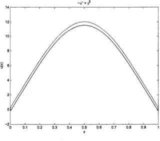
As a numerical example, we consider the following quadratic nonlinear two-point boundary

valueproblem [6]:

$\{\begin{array}{l}-u’’=u^{2} 0<x<1,u(0)=u(1)=0.\end{array}$ (22)

Anapproximate solution$\hat{u}$is calculated by the finite element method with

bases as

one-dimensional

piecewise linear hat functions. The proposal verification method is applicable to Eq. (22). Our

computer assisted proof method yields

$K=2.391,$ $L=0.005,$ $M=1.852$, $C_{1}=5.568,$ $C_{2}=0.059,$ $C_{3}=0.226$

.

Then we have $\alpha=0.333$ and $\omega=1.254$ so _that $\alpha\omega<0.417$

.

Consequently, it follows that there

exists an unique solutionin the ball $B(\hat{u}, \rho)$ with the radius

$\Vert u-\hat{u}\Vert_{H_{0}^{1}}\leq\rho=0.472$

.

Figure 1 shows the guaranteed inclusion of the exact solution of Eq. (22). It is proved that

there exists a unique solution between two

curves.

Since $H_{0}^{1}(0,1)arrow C^{0}(0,1)$, we can obtain the

guaranteed error bound in maximum norm by Poincar\’e$s$ inequality.

$x$

Figure 1: Guaranteed Inclusion ofthe Exact Solution (Mesh size $\frac{1}{512}$)

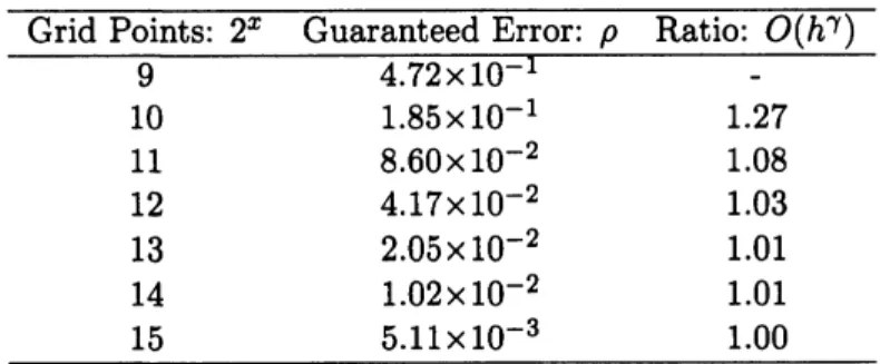
By increasing grid points, guaranteed error bounds are improved with $O(h)$

.

The guaranteed

error and the ratio are presented in Table 1. All computations are carried out on Mac OS X,

Intel Core2 Duo 1.$86GHz$ _by _{using MATLAB} $2009a$ with a toolbox for verified computations,

(13)

Table 1: VerificationResults for Problem (22) $\overline{\frac{GridPoints:2^{x}GuaranteedError:\rho Ratio:O(h^{\gamma})}{94.72\cross 10^{-1}-}}$ 10 $1.85\cross 10^{-1}$ 1.27 11 $8.60\cross 10^{-2}$ 1.08 12 $4.17\cross 10^{-2}$ 1.03

13

$2.05\cross 10^{-2}$ 1.01 14 $1.02\cross 10^{-2}$ 1.01 15 $5.11\cross 10^{-3}$ 1.00 References

[1] L. V. Kantorovich and G.P.Akilov, FunctionalAnalysis in Normed Spaces, translated from the

Russian by D. E. Brown, Pergamon Press, 1964.

[2] M.Urabe, Galerkin‘sprocedurefor nonlinear periodic systems, Arch.Rat. Mech. Anal. 20, 1965,

pp.120-152.

[3] M.A. McCarthy and R.A.Tapia, Computable

a

priori $L^{\infty}$

-error

bound for the approximate

solution of two-point boundary value problem,

SIAM

J. Numer. Anal. 12, 1975, pp.919-937.

[4] G. Kedem, A posteriori errorbounds for two-point boundary value problems, SIAM J. Numer.

Anal., 18, 1981, pp.431-448.

[5] M. T. Nakao, A numerical approach to the proof of existence of solutions for elliptic problems,

Japan Journal of Applied Mathematics 5, 1988, pp.313-332.

[6] M.T. NakaoandN. Yamamoto, NumericalVerification, Nihonhyouron-sya, 1998, (in Japanese).

[7] M. Plum, Computer-Assisted Existence Proofs forTwo-Point BoundaryValueProblems,

Com-puting 46, 1991, pp.19-34.

[8] R. A. Adams, Sobolev spaces, Academic Press, New York, 1975.

[9]

S.C.

Brenner and L.R. Scott, The MathematicalTheory ofFinite Element Methods, Springer, 2008.

[10] S. Oishi, Numerical verification of existence and inclusion of solutions for nonlinear operator

equations, Journal of Computational and Applied Mathematics (JCAM), 60, 1995, pp.171-185.

[11] S. Oishi, Numerical Methods with Guaranteed Accuracy, Corona-sya, 2000, (in Japanese).

[12] M. T.Nakao, K.Hashimoto and Y.Watanabe, Anumerical method to verify the invertibilityof

linear elliptic operators with applications tononlinear problems, Computing, 75, 2005, pp.1-14.

[13] S. Oishi, A. Takayasu, T. Kubo, Numericalverification of existence for solutions to Dirichlet

boundary value problems of semilinear elliptic equations, submitted to publication.

[14] S.M.Rump,INTLAB-INTerval LABoratory, aMatlab toolboxforverifiedcomputations,