The distributions of the sliding block patterns in finite samples and the inclusion-exclusion principles for partially ordered sets (Probability Symposium)
9
0
0
全文
(2) 2 It is well known that Monte Carlo simulation may generate a false distributions. In Section 4 we show. that Monte Carlo simulation with the BSD Library pseudo random number generator random (BSD RNG) and Mersenne twister pseudo random number generator (MT RNG). We show that BSD RNG computes a false distribution. The Monte Carlo simulation is itself considered to be a statistical test for. pseudo random numbers. In order to avoid a circular argument, we need to derive the distribution with mathematically assured manner.. The distributions of sliding block patterns have been shown via generating functions, see [4, 5, 1, 6, 7, 8]. Régnier and Szpankowski [5] derived generating functions of the sliding block patterns in a finite sample. In Goulden and Jackson [6] and Bassino et al [7], they obtained the distribution of the sliding block patterns with generating functions and inclusion‐exclusion method. The advantage of the method of. Bassino [7] is that the formula of generating functions are significantly simplified in combination with inclusion‐exclusion method. The formula of the generating function of the distribution of the sliding. block patterns in [4, 5, 1, 6, 7, 8] are based on the induction of sample size. In this paper we show the distributions of sliding block patterns for Bernoulli processes with finite alphabet, which is not based on the induction on sample size.. We show a new inclusion‐exclusion. formula in multivariate generating function form on partially ordered sets, and show a simpler expression of generating functions of the number of pattern occurrences in finite samples. We say that a word times, otherwise. w. is overlapping if there is a word. i.e., 11 appears 2 times in 111. We write x\sqsubset y if Theorem 1 Let. x. with |x|<2|w| and. P. be an. i.i.d .. x. is a prefix of. process of fixed sample size. n. an increasing non‐overlapping words of finite alphabet, i. e., is the length of. s_{i} ,. w. appears in. x. at least 2. is called non‐overlapping. For example 10 is non‐overlapping and 11 is overlapping,. w. y. and x\neq y.. of finite alphabet. Let s_{i}. for all i<j . Let P(s_{i}) be the probability of. s_{1}\sqsubset s_{2}\sqsubset.. ... s_{i}. for. i=1 ,. A(k_{1}, \ldots, k_{l})=(^{n-\sum_{\dot{i} m_{i}.k_{i}+\sum_{i}k_{i} k_{1}, . ,k_{l})\prod_{i=1}^{l}P^{k_{i} (s_{i}). be. \sqsubset s_{l}. is a prefix of s_{j} and m_{i}<m_{j} , where. m_{i}. . . . , l . Let. ,. B(k_{1}, \ldots, k_{l})=P(\sum_{i=1}^{n}I_{X_{\dot{i} ^{i+m_{i}-1}=s_{j} = k_{j}, j=1, \ldots, l). ,. (2). F_{A}(z_{1}, \ldots, z_{l})=\sum_{k_{1},\ldots,k_{l} A(k_{1}, \ldots, k_{l})z^ {k_{1} \cdots z^{k_{l} F_{B}(z_{1}, \ldots, z_{l})=\sum_{k_{1},\ldots,k_{l} B(k_{1}, \ldots, k_{l})z^ {k_{1} \cdots z^{k_{l} .. , and. Then. F_{A}(z_{1}, z_{2}, \ldots, z_{l})=F_{B}(z_{1}+1, z_{1}+z_{2}+1, \ldots, z_{1}+ \cdots+z_{l}+1). .. Or equivalently,. F_{A} (y_{1}-1, y_{2}-y_{1}, . . . y_{l}-y_{l-1})=F_{B}(y_{1}, y_{2}, . . . y_{l}) where y_{i}=z_{1}+\cdots+z_{i}+1 for. B(k_{1}, \ldots, k_{l}). i=1 ,. ...,. is the coefficient of the. ,. l.. \prod_{i=1}^{l}y_{\dot{i} ^{k_{\dot{i} }. in. F_{A}(y_{1}-1, y_{2}-y_{1}, \ldots, y_{l}-y_{l-1}). for all k_{1} , . . . , k_{l}..
(3) 3 It is known that in the case of one variable [9] or the multi‐variate disjoint events [7, 6, 4], inclusion‐ exclusion formula expressed via generating functions as F_{A}(z_{1}, \ldots, z_{l})=F_{B}(z_{1}+1, \ldots, z_{l}+1) , where F_{A} is a generation function for non‐sieved events and F_{B} is a generating function for sieved events.. Theorem 1 shows a new inclusion‐exclusion formula for partially ordered sets. With slight modification of Theorem 1, we can compute the number of the occurrence of the overlapping. increasing words. For example, let us consider increasing self‐overlapping words 11, 111, 1111 and the number of their occurrences. Let 011, 0111, 01111 then these words are increasing non‐self‐overlapping words. The number of occurrences 11, 111, 1111 in sample of length occurrences 011, 0111, 01111 in sample of length. n+1. n. that starts with. is equivalent to the number of 0.. In [5], expectation, variance, and CLTs (central limit theorems) for the sliding block pattern are shown. We show the higher moments for non‐overlapping words. Theorem 2 Let. w. be a non‐overlapping pattern. \min\{T,t\}. \foral tE(N_{w}^{t})= \sum_{s=1} A_{t,s}(\begin{ar ay}{l} n-s|w|+s S \end{ar ay})P^{s}(w) A_{t,s}= \sum_{r} (\begin{ar y}{l s r \end{ar y}) r^{t}(-1)^{s-r},. .. T= \max\{t\in \mathbb{N}|n-t|w|\geq 0\}.. In the above theorem, A_{t,s} is the number of surjective functions from \{ 1, 2, . . . , t\}arrow\{1,2, . . . , s\} for t, s\in \mathbb{N} ,. see [10].. The preliminary versions of the paper have been presented at [11, 12, 13, 14].. 2. Sparse Patterns In this section, we expand the notion of non‐overlapping patterns to sparse patterns. First we expand. the notion of non‐overlapping. Two words. w_{1}. such that |x|<|w_{1}|+|w_{2}| and. appear in. non‐overlapping. A set w_{1},. \mathcal{A}. S. w_{1}. and. w_{2}. and. w_{2}. are called non‐overlapping if there is no word x. . For example, the words 00101 and 00111 are. of words is called non‐overlapping if. w_{2}\in S including the case. w_{1}=w_{2}. x. w_{1}. and. w_{2}. are non‐overlapping for all. . We introduce the symbol? to represent arbitrary symbols. Let. be the alphabet. A word consists of extended alphabet \mathcal{A}\cup\{?\} is called sparse pattern. We say w' is. a realization of the sparse pattern. w. if w' consists of \mathcal{A} and coincides with. w. except for the symbol?.. A sparse pattern is called non‐overlapping if the set of the realization is non‐overlapping. For example 001?1 is a non‐overlapping sparse pattern and its realizations are 00101 and 00111 with \mathcal{A}=\{0,1\}. We can find many non‐overlapping sparse patterns. For example, each sparse pattern 0^{m+1}(1?^{m})^{n}1 is non‐overlapping for all. n,. m. . Here. w^{m}. is the. m. times concatenation of the word. w. . For example,. 0^{3}(1?^{2})^{2}1=0001??1??1. The probability of sparse pattern. w. is defined by. P(w)=w' \sum_{rea{\imath} ization} of wP(w') . We write. w_{1}\sqsubset w_{2}. for two sparse patterns if. holds for sparse words.. w_{1}. is a prefix of. w_{2}. with the alphabet \mathcal{A}\cup\{?\} . Theorem 1.
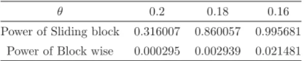
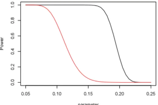
(4) 4 Corollary 1 Theorem 1 holds for non‐overlapping increasing. \mathcal{S}parse. patterns.. The advantage of the sparse patterns is that we can construct large size sparse patterns that have large probabilities, which is useful in statistical tests of pseudo random numbers in a large sample size.. 3. Experiments on power function of sliding block patterns tests In [5], it is shown that central limit theorem holds for sliding block patterns,. P( \frac{N_{w}-E(N_{w})}{\sqrt{V_{w} }<x)ar ow\frac{1}{\sqrt{2\pi} \int_{- \infty}^{x}e^{-\frac{ \imath} {2}x^{2} dx, where. w. is non‐overlapping pattern,. E(N_{w})=(n-|w|+1)P(w). and. V(N_{w})=E(N_{w})+(n-2|w|+2)(n-2|w|+1)P^{2}(w)-E^{2}(N_{w}) .. (3). Let. N_{w}':= \sum_{i=1}^{\lf o r n/|w|\rflo r}I_{x_{\dot{i}*|w|}^{(\dot{x}+1)*|w|- 1}=w}. N_{w}' obeys binomial law if the process is i.i. d . We call N_{w}'block-wi_{\mathcal{S}}e sampling. As an application of CLT approximation, we compare power functions of sliding block sampling N_{w} and block‐wise sampling N_{w}'.. We consider the following test for sliding block patterns: We write E_{\theta}=E(N_{w}) and V_{\theta}=V(N_{w}) if. P(w)=\theta . Null hypothesis: P(w)=\theta^{*} vs alternative hypothesis P(w)<\theta^{*}. Reject null hypothesis. if and only if N_{w}<E_{\theta^{*}}-5\sqrt{V_{\theta^{*}}} . The likelihood of the critical region is called power function, i.e.,. Pow(\theta) :=P_{\theta}(N_{w}<E_{\theta^{*}}-5\sqrt{V_{\theta^{*}}}). for \theta\leq\theta^{*}. We construct a test for block‐wise sampling: Null hypothesis: P(w)=\theta^{*} vs alternative hypothesis. P(w)<\theta^{*}. Reject null hypothesis if and only if. V_{\theta}'=\lfloor n/|w|\rfloor\theta(1-\theta). N_{w}'<E_{\theta^{*}}'-5\sqrt{V_{\theta^{*}}'} ,. where E_{\theta}'=\lfloor n/|w|\rfloor\theta and. .. The following table shows powers of sliding block patterns tests and block wise sampling at 0.2,0.18,0.16 under the condition that alphabet size is 2 (binary data), \theta^{*}=0.25, |w|=2 , and \theta. 0. 2. 0. 18. 0.16. Power of Sliding block. 0.316007. 0.860057. 0.995681. Power of Block wise. 0.000295. 0.002939. 0.021481. \theta=. n=500.. Figure 1 shows the graph of power functions for sliding block patterns test and block‐wise sampling..
(5) 5. \overlin{mathgL}\cireq. parameter. Figurel Comparison of power functions: sliding block test (black line) vs block‐wise test (red line). P(w)<0.25 vs P(w)=0.25 (null hypothesis). |w|=2, n=500.. 4. Experiments on statistical tests for pseudo random numbers In [15], a battery of statistical tests for pseudo random number generators are proposed, and chi‐. square test is recommended to test the pseudo random numbers with sliding block patterns N_{w} and. non‐overlapping word. w. . Expectation and variance of N_{w} are given in (3).. In this section, we apply Theorem 1 and Kolmogorov Smirnov test to pseudo random number gen‐. erators. Fix sample size. n=1600. following three distributions for 1. true distributions of. in (1) and null hypothesis. w=10. P. be fair coin flipping. We compute the. and 11110 in Figure 2.. N_{w},. 2. binomial distributions. (\begin{ar y}{l n k \end{ar y}) p^{k}(1-p)^{n-k}, p=2^{-|w|},. k=1 ,. 3. empirical distributions of. \sum_{i=1}^{n}I_{X_{i}^{i+|w|-1}=w}. ...,. n. , and. generated by Monte Carlo method with BSD RNG ran‐. dom, 200000 times iteration of random sampling. Due to the linearity of the expectation, the expectation of binomial distribution is pn, which is almost same to the expectation of N_{w} . However the random variables of sliding block patterns have strong correlations even if the process is i.i. d . For example, if a non‐overlapping pattern has occurred at some position, then the same non‐overlapping pattern do not occur in the next position.. From the graphs of distributions, we see that binomial distributions has large variance compared to the true distributions. This is because, in the binomial model, the correlations of patterns are not considered.. We see that the binomial model approximations of the distributions of the sliding block patterns are not appropriate.. Figure 2 shows that the empirical distributions (Monte Carlo method) is different from the true dis‐.
(6) 6 tribution. We see that BSD RNG random cannot simulate the sliding block patterns correctly.. \iota^{frc}LDdvelns_1\pim->. ’. \iota^{frc}LDds_\vapi^{1'equ>. 300. 350. 400. 450. 500. 0. 20. 40. Number of pattem occurences. Figure2 n=1600. 60. 80. 100. Number of pattem occurences. Comparison of distributions: the left graph shows the distributions for. and the right graph shows the distributions for. w=11110. and. n=1600. w=10. and. in (1). Black,. red, and blue lines show true distribution, binomial, and Monte Carlo simulation, respectively.. From the experiment for. we have obtained. w=11110. \sup |F_{t}(x)-F(x)|=0.302073,. 0\leq x<\infty. where F_{t}(x) is the empirical cumulative distribution generated by Monte Carlo method with BSD RNG. random with. t=200000. times random sampling.. Kolmogorov‐Smirnov theorem we have the. F(x) is the cumulative distributions of (2). From. p ‐value. P ( \sup |F_{t}(x)-F(x)|\geq 0.302513)\approx 0, 0\leq x<\infty. where. P. is the fair coin flipping (null hypothesis). The sliding block patterns tests reject BSD RNG. random. The 200000 and. p ‐values. n=1600. of the Kolmogorov‐Smirnov test for BSD RNG with w=10,. w=11110,. t=. are summarized in the following table. BSD RNG. w=10. w=11110. \sup_{0\leq x<\infty}|F_{t}(x)-F(x)|. 0.012216. 0.302073. p ‐value. 0. 0. The sliding block patterns tests do not reject MT RNG [16] under the same condition above. The p‐ values of the Kolmogorov‐Smirnov test for MT RNG with w=10, w=11110, are summarized in the following table. MT RNG. w=10. w=11110. \sup_{0\leq x<\infty}|F_{t}(x)-F(x)|. 0.001376. 0.001409. p ‐value. 0.843306. 0.822066. t=200000. and. n=1600.
(7) 7. 5. Proofs Proof of Theorem 1) For simplicity we give a proof for the case of two non‐overlapping words. w_{1}\sqsubset w_{2}. in Theorem 1. The proof of the general case is similar. Let m_{1}=|w_{1}| and m_{2}=|w_{2}| . Since w_{2}. are non‐overlapping, the number of possible allocations such that k_{1} times appearance of. times appearance of. w_{2}. in the string of length. n. n. w_{1}. and. w_{2}. and. and k_{2}. .. with additional two extra symbols. \alpha,. \beta in the string of length. then the problem reduces to choosing k_{1}\alpha ’s and k_{2}\beta ’s among string of length n-m_{1}k_{1}-m_{2}k_{2}+k_{1}+k_{2}.. In the above equation, we do not count the appearance of. w_{1}. in. w_{2}. . Let. A(k_{1}, k_{2})=(\begin{ar ay}{l} n-m_{1}k_{1}-m_{2}k_{2}+k_{1}+k_{2} k_{1},k_{2} \end{ar ay}) P^{k_{ \imath} }(w_{1})P^{k_{2} (w_{2}) A. w_{1}. is. (\begin{ar ay}{l} n-m_{1}k_{1}-m_{2}k_{2}+k_{1}+k_{2} k_{1)}k_{2} \end{ar ay}) This is because if we replace each. w_{1}. .. is not the probability that k_{1}w_{1} ’s and k_{2}w_{2} ’s occurrence in the string, since we allow any words in. the remaining place of the string except for the appearance of the event that. and. w_{1}. non‐overlapping words. w_{2} w_{1}. w_{1}. and. w_{2} .. For example. A. may count. appear more than k_{1} and k_{2} times. Let B(t_{1}, t_{2}) be the probability that. and. w_{2}. appear k_{1} and k_{2} times respectively. We have the following identity,. A(k_{1}, k_{2})=k_{2} \leq t_{2},\sum_{k_{1}+k_{2}\leq t_{1}+t_{2} B(t_{1}, t_{2}) (\begin{ar y}{l t_{2} k_{2} \end{ar y}) \sum_{0\leq s\leq t_{2}-k_{2} (\begin{ar ay}{l t_{2}-k_{2} s \end{ar ay})(\begin{ar ay}{l t_{1} k_{1}-s \end{ar ay}) . Let F_{A}(z_{1}, z_{2}). tions for. A. and. := \sum_{k_{{\imath}},k_{2}}A(k_{1}, k_{2})z^{k_{1}}z^{k_{2}} B. and F_{B}(z_{1}, z_{2}). := \sum_{k_{{\imath}},k_{2}}B(k_{1}, k_{2})z^{k_{1}}z^{k_{2}}. (4). be generating func‐. respectively. From (4), we have. F_{A}(z_{1}, z_{2})= \sum_{k_{1},k_{2} z_{1}^{k_{1} z_{2_{k_{2}\leq t_{2} }^{k_ {2} ,\sum_{k_{1}+k_{2}\leq t_{1}+t_{2} B(t_{1}, t_{2}) (\begin{ar y}{l t_{2} k_{2} \end{ar y}) \sum_{0\leq,\leq t_{2}-k_{2} (\begin{ar ay}{l t_{2}-k_{2} s \end{ar ay})(\begin{ar ay}{l t_{l} k_{1}-s \end{ar ay}) = \sum_{t_{ \imath} ,t_{2} B(t_{1}, t_{2})\sum_{k_{2}\leq t_{2} (\begin{ar y}{l t_{2} k_{2} \end{ar y}) z_{2}^{k_{2} \sum_{0\leq s\leq t_{2}-k_{2},0\leq k_{1}-s\leq t_{1} (\begin{ar ay}{l t_{2}-k_{2} s \end{ar ay})(\begin{ar ay}{l t_{1} k_{1}-s \end{ar ay}) z_{1}^{k_{1} = \sum_{t_{ \imath} ,t_{2} B(t_{1}, t_{2})\sum_{k_{2}\leq t_{2} (\begin{ar y}{l t_{2} k_{2} \end{ar y}) z_{2}^{k_{2}}(z_{1}+1)^{t_{1}+t_{2}-k_{2}}. = \sum_{t_{ \imath} ,t_{2} B(t_{1}, t_{2})(z_{1}+1)^{t_{1}+t_{2} (\frac{z_{2} {z_{1}+1}+1)^{t_{2} =F_{B}(z_{1}+1, z_{1}+z_{2}+1). .. In the above second equality, we changed the order of summation of variables. The latter part of the theorem is obvious.. Proof of Theorem 2) For simplicity ıet i=j. Y_{\dot{i}}Y_{j}=0 if. \blacksquare. Y_{\dot{i}}=I_{X_{i}^{i+|w-1}}.=w .. Since. w. is non‐overlapping, Y_{\dot{i}}Y_{j}=Y_{\dot{i}} if. \{i, i+1, . . . , i+|w|-1\}\cap\{j, j+1, . . . , j+|w|-1\}\neq\emptyset . We say that \{i, i+1, . . . , i+|w|-1\}. is the coordinate of Y_{i} . We say that a subset of. \{Y_{i}\}_{1\leq i\leq n-|w|+1} is disjoint if their coordinate are disjoint..
(8) 8 Let Yí, j=Y_{i} for all 1\leq j\leq t .. E( \prod_{\dot{j}=1}^{t}Y_{i,j})=P^{S}(w). Then. ( \sum_{i}Y_{i})^{t}=\prod_{\dot{j}=1}^{t}\sum_{i}Y_{i,j}=\sum_{i}\prod_{j=1} ^{t}Y_{\dot{i}j} .. if and only if there is a disjoint set Y_{n(j)}, 1\leq j\leq s such that. Note that. \prod_{j=1}^{t}Y_{\dot{i}j}=. \prod_{\dot{J}^{=1}}^{s}Y_{n(j)}. Observe that the number of possible combination of disjoint sets of Y_{n(j)}, 1\leq j\leq s such that. A_{t,s}(^{n-s|_{S}w|}+s) s> \max\{t\in \mathbb{N}|n-t|w|\geq 0\} \prod_{j=1}^{t}Y_{\dot{i}j}=\prod_{j=1}^{s}Y_{n(j)}. is. . Note that there is no disjoint sets of Y_{n(j)}, 1\leq j\leq s if. . From the linearity of the expectation, we have the theorem. \blacksquare. Acknowledgment The author thanks for a helpful discussion with Prof. S. Akiyama and Prof. M. Hirayama at Tsukuba University. This work was supported by the Research Institute for Mathematical Sciences, an Interna‐. tional Joint Usage/Research Center located in Kyoto University, and Ergodic theory and related fields in Osaka University.. References [1] P. Jacquet and W. Szpankowski, Analytic Pattern Matching. [2] P. Shields, The ergodic theory of discrete sample paths.. Cambridge University Press, 2015.. Amer. Math. Soc., 1996.. [3] M. Li and P. Vitányi, An introduction to Kolmogorov complexity and Its applications, 3rd ed.. New. York: Springer, 2008.. [4] L. Guibas and A. Odlyzko, “String overlaps, pattern matching, and nontransitive games. J. Com‐. bin. Theory Ser. A, vol. 30, pp. 183‐208, 1981.. [5] M. Régnier and W. Szpankowski, (On pattern frequency occurrences in a markovian sequence Algorithmica, vol. 22, no. 4, pp. 631‐649, 1998.. [6] I. Goulden and D. Jackson, Combinatorial Enumeration.. John Wiley, 1983.. [7] F. Bassino, J. Clément, and P. Micodème, “Counting occurrences for a finite set of words: combi‐ natorial methods. ACM Trans. Algor., vol. 9, no. 4, p. Article No. 31, 2010.. [8] P. Flajolet and R. Sedgewick, Analytic Combinatorics. [9] H. S. Wilfl, Generatingfunctionlogy, 3rd ed.. Cambridge University Press, 2009.. CRC press, 2005.. [10] J. Riordan, Introduction to combinatorial analysis.. John Wiley, 1958.. [11] H. Takahashi, “Inclusion‐exclusion principles on partially ordered sets and the distributions of the number of pattern occurrences in finite samples. pp. 5‐6, Sep. 2018, mathematical Society of Japan,. Statistical Mathematics Session, Okayama Univ. Japan.. [12] —, “The distributions of the sliding block patterns in finite samples. Nov. 2018, ergodic Theory. and Related Fields, Osaka Univ. Japan.. [13] —, “The distributions of sliding block patterns in finite samples and the inclusion‐exclusion principles for partially ordered sets. Dec. 2018, probability Symposium, Kyoto Univ. Japan. arxiv:1811.12037v1.. [14] —, “The distributions of the sliding block patterns. Dec. 2018, pp. 223‐225, the 41st Symposium.
(9) 9 on Information Theory and Its Applications (SITA2018) Iwaki, Fukushima, Japan. [15] A. Rukhin, J. Soto, J. Nechvtal, M. Smid, E. Barker, S. Leigh, M. Levenson, M. Vangel, D. Banks, A. Heckert, J. Dray, and S. Vo, A statistical Test Suite for Random and Pseudorandom Number. Generators for Cryptographic Applications, NIST Special Publication. 80\theta-22. Revised la, US, 2010.. [16] M. Matsumoto and T. Nishimura, “Mersenne twister: A 623‐dimensionally equidistributed uniform pseudorandom number generator pp. 3‐30, Jan 1998.. ACM Trans. on Modeling and Computer Simulation, vol. 8, no. 1,.
(10)
図
関連したドキュメント
In this partly expository article we show, from the perspective of partially ordered sets, that the family of connected threshold graphs is isomorphic to the lattice of shifted
Keywords: composition, factor order, finite state automaton, generating function, partially ordered set, rationality, transfer matrix, Wilf equivalence.. Dedicated to Anders Bj¨orner
If condition (2) holds then no line intersects all the segments AB, BC, DE, EA (if such line exists then it also intersects the segment CD by condition (2) which is impossible due
We recall here the de®nition of some basic elements of the (punctured) mapping class group, the Dehn twists, the semitwists and the braid twists, which play an important.. role in
Then it follows immediately from a suitable version of “Hensel’s Lemma” [cf., e.g., the argument of [4], Lemma 2.1] that S may be obtained, as the notation suggests, as the m A
Definition An embeddable tiled surface is a tiled surface which is actually achieved as the graph of singular leaves of some embedded orientable surface with closed braid
The crucial assumption in [14] is that the distribution of the increments possesses a density and has an everywhere finite moment-generating function. In particular, the increments
Moreover, by (4.9) one of the last two inequalities must be proper.. We briefly say k-set for a set of cardinality k. Its number of vertices |V | is called the order of H. We say that
