2009, Vol. 52, No. 2, 163-173
SELECTING INPUTS AND OUTPUTS IN DATA ENVELOPMENT ANALYSIS BY DESIGNING STATISTICAL EXPERIMENTS
Hiroshi Morita Necmi K. Avkiran
Osaka University The University of Queensland
(Received March 19, 2008; Revised August 12, 2008)
Abstract Data envelopment analysis (DEA) is a data oriented, non-parametric method to evaluate relative efficiency based on pre-selected inputs and outputs. In some cases, the performance model is not well defined, so it is critical to select the appropriate inputs and outputs by other means. When we have many potential variables for evaluation, it is difficult to select inputs and outputs from a large number of possible combinations. We propose an input output selection method that uses diagonal layout experiments, which is a statistical approach to find an optimal combination. We demonstrate the proposed method using financial statement data from NIKKEI 500 index.
Keywords: DEA, fractional factorial design, Mahalanobis distance
1. Introduction
Evaluation of performance is an important activity in identifying shortcomings in manage-rial efficiency and devising goals for improvement. Many activities can be expressed as a translation of inputs to outputs, where it is desirable to produce more outputs with less inputs. Data envelopment analysis (DEA), the most representative method for efficiency evaluation, is a mathematical programming method for evaluating the relative efficiency of decision making units (DMUs) with multiple inputs and multiple outputs.
DEA is a data-oriented non-parametric method. A production possibility set is con-structed empirically by enveloping the inputs and outputs data set, where a parametric transformation function is not assumed. The efficient frontier of a production possibility set enables the relative efficiency evaluation. The efficiency score distinguishes between efficient and inefficient DMUs by establishing whether a DMU is located on the efficient frontier or inside the production possibility set. Also, the efficiency score indicates how far a DMU is from the efficient frontier.
DEA empirically identifies the efficient frontier of a set of DMUs based on the input and output variables. Assume that there are n DMUs, and the jth DMU, DMUj, produces s
outputs (yij, ..., ysj) by using m inputs (x1j, ..., xmj). The efficiency score of the observed
DMUo is given as the optimal value to the following linear programming problem:
θ∗o = min θ s.t.∑ j λjxij ≤ θxio, i = 1, ..., m ∑ j λjyrj ≥ yro, r = 1, ..., s λj ≥ 0, j = 1, ..., n (1.1)
This is an input oriented constant returns to scale (CRS) model. The efficiency of DMUo
is determined from efficiency score θ∗o and its slack values. If θ∗o = 1 and there is no slack, DMUo is said to be efficient. If θo∗ = 1 and there are non-zero slacks, DMUo is inefficient
and is called to be weak-efficient. The weak-efficient DMUs and efficient DMUs comprise the efficient frontier.
Evaluation based on the efficiency score is directly affected by the input and output variables. That is, the inputs and outputs should be selected appropriately so as to express the performance of DMUs. For instance, the selection may be founded on a particular theory, e.g. production versus intermediation approaches to bank behavior. Alternatively, expert knowledge or accepted practices can be useful in determining the variables. For example, when we assess the profit efficiency of banks, two inputs (interest expense and non-interest expense) and two outputs (interest income and non-interest income) are often used as the core variables [6]. However, stakeholders in bank performance would interpret measures differently when it comes to categorizing a variable as an input or an output. This is due to the variety of stakeholders. We normally treat variables considered to be desirable as outputs, and those considered to be undesirable are treated as inputs. For instance, a head office executive would be more interested in running the organization with a smaller number of employees, whereas a branch manager may be interested in having more employees at the disposal of the branch. That is, number of employees is likely to be an undesirable attribute (i.e. an input) for the executive and a desirable attribute (i.e. an output) for the branch manager, which may lead the hesitation to decide input or output to evaluate overall efficiency [10].
Furthermore, in some cases, the performance measure is not always clearly defined. For example, in evaluating baseball players, there are many variables which can be used to capture a player’s performance. Hirotsu and Ueda [7] use seven outputs such as rate of home runs, rate of runs batted in, rate of stolen bases, batting average, slugging percentage, on-base percentage, and batting average in scoring position. But it is possible to use other variables such as at bats, strikeouts, sacrifice bunts, annual salary and so on. Thus, it is necessary to select a parsimonious set of inputs and outputs so as to capture the performance of a DMU’s key activities.
DEA framework identifies the non-dominated efficient DMUs in the data space spanned by inputs and outputs. So, too many inputs and outputs manifest as too many relatively efficient DMUs. Similarly, too few inputs and outputs cannot show the efficient DMUs. Therefore, it is desirable to develop a mathematical approach to selecting input and output variables for performance evaluation that will distinguish between efficient and inefficient DMUs, particularly where appropriate theory or accepted practices are not available.
In a previous study, Morita and Haba [3] select outputs so as to distinguish between two groups based on external information, where a 2-level orthogonal layout experiment is utilized and optimal variables can be found statistically. On the other hand, Ediridsinghe and Zhang [4] have proposed a generalized DEA approach to select inputs and outputs by maximizing the correlation between the DEA score and the external performance index. They utilize a two-step heuristic algorithm that combines random sampling and local search to find an optimal combination of inputs and outputs.
In this paper, we consider an input and output selection method based on discriminant analysis using external evaluation. We use a 3-level orthogonal layout experiment to find an appropriate combination of inputs and outputs, where experiments are independent of each other.
selection method using the 2-level layout experiment proposed in [3]. Then, the method of variable selection is expanded in section 3 through a 3-level orthogonal layout experiment, where inputs as well as outputs are considered. A case study of management efficiency of ranked Japanese companies is demonstrated in section 4. Section 5 concludes the paper.
2. Selecting Output Variables Using a 2-Level Fractional Factorial Design
We select the appropriate output variables so as to distinguish between two groups, that is, high performers and low performers, on efficiency scores [3]. We assume that external performance criteria on high performers and low performers are available. The distance between the two groups is measured by the Mahalanobis distance. In this study, we consider the distance of one-dimensional variables, where Mahalanobis distance coincides with the Welch statistics. The Welch statistics is given as
d = ¯ θh− ¯θl √ Vh nh + Vl nl (2.1)
where the mean and variance of each group are given as ¯θh, Vh for nh high performers and
¯
θl, Vl for nl low performers.
The aim is to find that combination of output variables which maximizes the distance d. In our first example, for simplicity, we utilize the 2-level factorial design. When there are k candidates of output variables, the total number of combinations is 2k. Full factorial designs perform all of 2k combinations for k candidates. On the other hand, we can define a 2k−p
design to be a fractional factorial design with k candidates, each at two levels, consisting of 2k−p runs. The first (k− p) candidates are part of 2k−p combinations as a full factorial design, and the remaining p candidates can be generated as interactions with the first (k−p) columns. Table 1 shows the example of a fractional factorial design where k = 5, p = 2, and xi is a candidate variable. ’+’ means that the variable is selected as an output, and ’−’
means that the variable is not selected as an output. For example, the variables x1, x3, x4
are selected as outputs in run No. 3.
Based on the fractional factorial design in Table 1, we calculate the efficiency scores by (1.1) Table 1: Fractional factorial design for 25−2 and selected outputs
Runs x1 x2 x3 x4 x5 Selected Outputs Mahalanobis distance
1 + + + + + x1, x2, x3, x4, x5 d1 2 + + − − − x1, x2 d2 3 + − + + − x1, x3, x4 d3 4 + − − − + x1, x5 d4 5 − + + − − x2, x3 d5 6 − + − + + x2, x4, x5 d6 7 − − + − + x3, x5 d7 8 − − − + − x4 d8
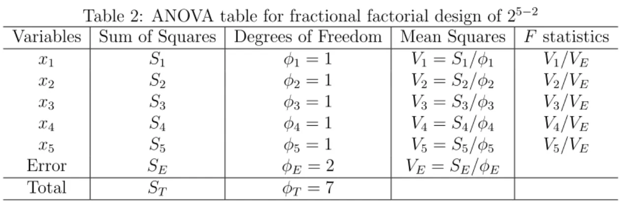
and Mahalanobis distance by (2.1) between two groups using the selected output variables. The analysis of variance (ANOVA) for the fractional factorial design appears in Table 2.
The total sum of squares ST is given as
ST = 8
∑
i=1
Table 2: ANOVA table for fractional factorial design of 25−2
Variables Sum of Squares Degrees of Freedom Mean Squares F statistics
x1 S1 φ1 = 1 V1 = S1/φ1 V1/VE x2 S2 φ2 = 1 V2 = S2/φ2 V2/VE x3 S3 φ3 = 1 V3 = S3/φ3 V3/VE x4 S4 φ4 = 1 V4 = S4/φ4 V4/VE x5 S5 φ5 = 1 V5 = S5/φ5 V5/VE Error SE φE = 2 VE = SE/φE Total ST φT = 7
The sum of squares Si for candidate i reflects the main effect of the variable, which is the
difference between ’+’ and ’−’ as,
Si = 2{ ¯d(xi+)− ¯d(xi−)}2 (2.3)
where ¯d(xi+) is the mean of the Mahalanobis distances observed when xi = +. The residual
sum of squares SE is given by subtracting the sum of Si from ST.
SE = ST − (S1+ S2+ S3+ S4+ S5) (2.4)
The total degree of freedom is φT = 7, which is the number of runs minus 1, and the degree
of freedom for each sum of squares is φi = 1. Therefore the degree of freedom for the residual
is given as,
φE = φT − (φ1+ φ2 + φ3+ φ4+ φ5) = 2 (2.5)
The null hypothesis that the candidate has no effect as an output is tested by using the F statistics,
F = Si/φi SE/φE
. (2.6)
The test rejects the null hypothesis at level α if F -value exceeds α percentile of F distribution with degrees of freedom (φi, φE).
The negligible variables are pooled into the residual and the remaining variables should be selected as outputs. Then, we can obtain the optimal combination of output variables.
The following summarize the procedure for variable selection. Step 1. List potential input output variables.
Step 2. Use external criteria to distinguish the performance of two groups, e.g. high and low performers.
Step 3. Assign the variables to an orthogonal layout and determine the combination of selected variables used in the experiments.
Step 4. Calculate the DEA efficiency scores and Mahalanobis distance between the two groups by using the selected variables.
Step 5. Determine the optimal combination of input output variables based on results of analysis of variance.
Step 6. Identify the optimal designation of statistically significant variables as either an input or an output using Mahalanobis distance.
3. Selecting Input and Output Variables Using a 3-Level Fractional Factorial Design
When a variable is considered for DEA, it is necessary to determine whether the variable should act as an input or an output. Some variables can be pre-specified as inputs or outputs based on the production conversion mechanism of a DMU or the expert knowl-edge of the analyst. When it is difficult to understand the conversion mechanism, inputs and outputs should be determined endogenously. Here, we obtain the efficiency measure to distinguish between high-performing DMUs and low-performing DMUs by selecting an appropriate combination of inputs and outputs that maximizes the distance d between the two groups. When there are k candidates of variables in a 3-level design, the total number of possible input and output combinations rises to 3k. Full factorial designs perform all of 3k
combinations. We can define a 3k−pfractional design with k candidates, each at three levels, consisting of 3k−p runs. Table 3 shows this fractional factorial design when k = 3, p = 1,
where ’1’ means that the variable is selected as an input, ’2’ means that the variable is selected as an output, and ’3’ means that the variable is not selected. For example, in run No. 4, variable x2 is selected as an input and variable x1 is selected as an output; variable
x3 is not selected as an input or an output. When no output (input) is selected (e.g. see
runs 1 and 6), constant output (input) is assumed, i.e. unity.
Based on the fractional factorial design in Table 3, we calculate the efficiency scores and
Ma-Table 3: Fractional factorial design for 33−1 and selected inputs and outputs Runs x1 x2 x3 Selected Inputs Selected Outputs Distance
1 1 1 1 x1, x2, x3 None d1 2 1 2 2 x1 x2, x3 d2 3 1 3 3 x1 None d3 4 2 1 3 x2 x1 d4 5 2 2 1 x3 x1, x2 d5 6 2 3 2 None x1, x3 d6 7 3 1 2 x2 x3 d7 8 3 2 3 None x2 d8 9 3 3 1 x3 None d9
halanobis distance between the two groups using selected inputs and outputs. The ANOVA table for the fractional factorial design appears in Table 4.
The sum of squares and the degrees of freedom are given as,
Table 4: ANOVA table for fractional factorial design of 33−1
Variables Sum of Squares Degrees of Freedom Mean Squares F statistics
x1 S1 φ1 = 2 V1 = S1/φ1 V1/VE
x2 S2 φ2 = 2 V2 = S2/φ2 V2/VE
x3 S3 φ3 = 2 V3 = S3/φ3 V3/VE
Error SE φE = 2 VE = SE/φE
ST = 9 ∑ i=1 (di− ¯d)2, φT = 8 (3.1) Si = 3{ ¯d2(xi = 1) + ¯d2(xi = 2) + ¯d2(xi = 3)} − 9 ¯d2, φi = 2 (3.2) SE = ST − (S1+ S2 + S3), φE = φT − (φ1+ φ2+ φ3) = 2 (3.3)
where ¯d(xi = 1) is the mean of the Mahalanobis distances observed when xi = 1. The null
hypothesis that the candidate has no effect as an input or output is tested by using the F statistics.
The negligible variables are pooled into the residual. A statistically significant variable may be considered as an input or an output based on the maximum returned by { ¯d(xi =
1), ¯d(xi = 2), ¯d(xi = 3)}. If ¯d(xi = 1) is the maximum, variable xi should be an input. If
¯
d(xi = 2) is the maximum, then variable xi should be an output. On the other hand, if
¯
d(xi = 3) is the maximum, variable xi should not be an input or an output. This results in
the optimal combination of input and output variables.
4. A Case Study of Management Efficiency Using Financial Data
We use the NIKKEI 500 (2007), which is a ranking based on financial data. Ranking is based on the following four dimensions, which are given by fifteen indexes entered into factor analysis, where the result is converted into a score in the range 0-100.
(i) Scale: sales, owners’ equity, number of employees, cash flow
(ii) Profitability: ratio of sales to operating income, return on equity, rate of return on total assets
(iii) Safety: debt-to-asset ratio, interest coverage ratio, net interest expense to sales ratio, liquidity ratio
(iv) Growth: growth rates of total assets, sales, number of employees, and owners’ equity. In Step 1 (see Section 2), the following twelve variables are collected to evaluate the managerial performance of companies. Table A1 in the Appendix shows a part of the data set. Most of these variables except for (J) and (K) have large coefficients of variation (CV), that is, the standard deviation is greater than the mean.
(A) Issued stocks (B) Market price (C) Total assets (D) Capital
(E) Cash flow (F) Total sales (G) Ordinary profits (H) Net profits
(I) Number of employees (J) Return of equity (K) Sales to profits ratio
(L) Debt ratio
In Step 2, we construct two groups, high-performers and low-performers, from the top-ranked 30 and bottom-top-ranked 30 companies. Table A1 shows the mean and standard devi-ation for each variable. The varidevi-ation among the companies is quite large, even though we are focusing on top and bottom performers. When we select the variables to capture the
difference between high-performers and low-performers, we choose a variable with a large difference between these two groups. Mahalanobis distance between the top 30 and bottom 30 for each variable is also shown in Table A1, where we find that (B), (D), (G), (H) and (I) have a large d and may be intuitively selected as inputs or outputs.
In Step 3, we assign twelve factors into a three-level orthogonal layout, where at least twenty-seven runs are required. That is, we utilize the fractional factorial design 312−9.
Table 5 shows the selected variable combinations for efficiency score calculation. The Ma-halanobis distance for each experiment is calculated in Step 4, which is also shown in the last column of Table 5.
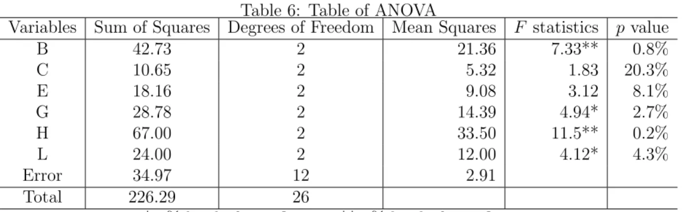
Table 6 shows the analysis of variance for the data in Table 5, where we have pooled the
Table 5: Selected inputs and outputs and Mahalanobis distance
No Inputs Outputs d 1 A, B, C, D, E, F, G, H, I, J, K, L None −5.87 2 A, B, C, D E, F, G, H, I, J, K, L 1.62 3 A, B, C, D None −4.31 4 A, E, F, G B, C, D, H, I, J 0.75 5 A, K, L B, C, D, E, F, G 2.72 6 A, H, I, J B, C, D, K, L 0.09 7 A, E, F, G K, L −6.06 8 A, H, I, J E, F, G 0.25 9 A, K, L H, I, J 3.34 10 B, E, H, K A, C, F, I, L −3.08 11 B, G, J A, C, E, H, K 0.35 12 B, F, I, L A, C, G, J 2.12 13 D, E, J, L A, B, F, H 4.37 14 D, G, I, K A, B, E, J, L −1.12 15 D, F, H A, B, G, I, K 0.01 16 C, E, I A, D, F, J, K −5.43 17 C, G, H, L A, D, E, I −1.91 18 C, F, J, K A, D, G, H, L 0.74 19 B, E, H, K D, G, J −2.21 20 B, F, I, L D, E, H, K 0.79 21 B, G, J D, F, I, L −2.52 22 C, E, I B, G, H, L 2.41 23 C, F, J, K B, E, I 3.19 24 C, G, H, L B, F, J, K 1.00 25 D, E, J, L C, G, I, K 2.53 26 D, F, H C, E, J, L −3.47 27 D, G, I, K C, F, H 3.17
negligible variables into the residual (step 5). The level of significance is shown as the p value, where we find four variables (B, G, H and L) significant at the 5% level. The variables (C) and (E) are not significant at the 5% level, but since their p values are not very high, we leave them in the analysis for illustrative purposes.
Step 6, the final step in our procedure, generates Table 7 which shows the means of Ma-halanobis distance for each variable at each level. For example, when variable B is selected
Table 6: Table of ANOVA
Variables Sum of Squares Degrees of Freedom Mean Squares F statistics p value
B 42.73 2 21.36 7.33** 0.8% C 10.65 2 5.32 1.83 20.3% E 18.16 2 9.08 3.12 8.1% G 28.78 2 14.39 4.94* 2.7% H 67.00 2 33.50 11.5** 0.2% L 24.00 2 12.00 4.12* 4.3% Error 34.97 12 2.91 Total 226.29 26
* 5% level of significance; ** 1% level of significance
as an input, the mean of Mahalanobis distance is −1.457, and when variable B is selected as an output, d is 1.491; when variable B is not selected, d is −0.760. Thus, given that the largest d for variable B is 1.491, it should be selected as an output. Maxima are indicated in bold font in Table 7. Thus, we select one input (L) debt ratio, and four outputs, namely, (B) market price, (C) total asset, (G) ordinary profits and (H) net profits. We run the DEA model (1) using this input and output combination, and obtain a Mahalanobis distance of 7.42.
Based on the selected inputs and outputs, we analyze the effectiveness of efficiency eval-Table 7: Mahalanobis distance means
Variables Selected as input Selected as output Not selected
B −1.457 1.491 −0.760 C −0.951 0.576 −0.350 E −1.399 0.269 0.404 G −1.357 1.132 −0.501 H −1.688 1.949 −0.987 L 1.010 −1.266 −0.470
uation through stratification [5]. Stratification consists of generating a tiered structure of multiple efficient frontiers. That is, Tier 1 represents the original efficient frontier with the full sample. We create Tier 2 when we remove the Tier 1 efficient DMUs and re-run DEA. To create Tier 3, Tier 2 efficient DMUs are removed, and so on. Twenty-two tiers emerge once our sample is exhausted by the stratification procedure. Figure 1 shows the numbers of companies in each tier. The companies in top 30 are categorized into the higher tiers and the companies in bottom 30 are categorized into the lower tiers. We accept this finding as empirical evidence that the selected input output combination effectively distinguishes between the two groups.
When we have many variables to evaluate performance, we may consider using all of them. In this study, there are twelve variables. At face value, the variables (I) and (K) have a ’smaller-the-better’ characteristic and the others have a ’larger-the-better’ characteristic. Table 8 summarizes the Mahalanobis distances and average efficiency scores for several combinations. Initially, we demonstrate using all the variables as per earlier prima facie selection of inputs and outputs, i.e. Case (a). For Case (a), there are too many outputs, many companies are evaluated to be efficient and as a result, we cannot distinguish between the two groups. Case (b) represents the combination that returned the maximum distance
Figure 1: Distribution of companies for each tier after stratification
among the previously calculated twenty-seven runs (see run 13 in Table 5) but it is not optimal either. Finally, the combination to emerge from our proposed method is shown in Case (c), where the Mahalanobis distance is maximized, and the efficiency differences between the two groups are better highlighted.
We apply linear discriminant analysis to the same data set, where seven variables (B, D,
Table 8: Efficiency scores and Mahalanobis distance
Mahalanobis Top 30 Bottom 30 Case Inputs Outputs distance Ave. s. d. Ave. s. d.
(a) I, K A, B, C, D, E, F, G, H, J, L −0.09 0.597 0.312 0.604 0.278 (b) D, E, J, L A, B, F, H 4.37 0.784 0.213 0.480 0.316 (c) L B, C, G, H 7.42 0.394 0.278 0.016 0.013
E, I, J, K and L) appear in the discriminant function. Based on the sign of coefficients of the linear discriminant function, the company having large values for two variables (E and L) and small values for five variables (B, D, I, J and K) will be classified into the top group. Then, the emerging Mahalanobis distance between the two groups, 6.24, is smaller than 7.42 obtained by our method. The number of misclassifications is 7 companies using discriminant analysis, but Figure 1 shows reversed evaluation for only 2 companies.
5. Concluding Remarks
We have considered an input output selection method that utilizes a 3-level fractional facto-rial design, Mahalanobis distance and ANOVA. The concept of discriminant analysis is used to distinguish between the two groups (Top30 and Bottom30), where the efficiency score is utilized as a one-dimensional measure. Variables are selected from the results of ANOVA to maximize the Mahalanobis distance between two groups. We can find an effective variable combination from a limited number of experiments. We demonstrate the effectiveness of this new approach using a case study with Japanese ranked companies. The selected inputs and outputs measure the performance efficiency that can effectively distinguish between the groups of high and low performers.
The obtained combination is not always optimal when estimated from a limited number of experiments. The orthogonal layout executes fractional combinations of experiments and is assigned selected interactions when necessary. Missing interactions may not lead to a good result, so it is necessary to provide the appropriate interactions. Moreover, the underlying assumptions on error terms such as normality, additivity, and homogeneity may be critical. We acknowledge that results may be unstable in the case of a changed assignment of columns or interactions. If it is essential to have a stronger optimality, combinatorial optimization techniques [9] such as branch and bound methods, or meta-heuristic methods can be applied. References
[1] W.W. Cooper, L.M. Seiford and K. Tone: Data Envelopment Analysis (Kluwer Aca-demic Publishers, 2000).
[2] G. Taguchi, Y. Wu and S. Chowdhury: Mahalanobis-Taguchi System (McGraw-Hill Professional, 2000).
[3] H. Morita and Y. Haba: Variable selection in data envelopment analysis based on external information. Proceedings of the eighth Czech-Japan Seminar 2005 on Data Analysis and Decision Making under Uncertainty, (2005), 181–187.
[4] N.C.P. Edirisinghe and X. Zhang: Generalized DEA model of fundamental analysis and its application to portfolio optimization. Journal of Banking & Finance, 31 (2007), 3311–3335.
[5] L.M. Seiford and J. Zhu, Context-dependent data envelopment analysis: measuring attractiveness and progress. Omega, 31 (2003), 397–408.
[6] N.K. Avkiran and H. Fukuyama: An illustration of network SBM with simulated profit centre data for Japanese regional banks. Proceedings of DEA Symposium 2008 (2008), 13–22.
[7] N. Hirotsu and T. Ueda: An evaluation of diversity in DEA. Proceedings of DEA Symposium 2008 (2008), 108–111.
[8] C. F. Jeff Wu and M. Hamada: Experiments – Planning, Analysis, and Parameter Design Optimization (John Wiley & Sons, Inc., 2000).
[9] D. Z. Du and P. M. Pardalos: Handbook on Combinatorial Optimization (Springer, 1999).
[10] N. K. Avkiran and H. Morita: Predicting bank stock performance with a model of fundamental relative analysis (in submission).
Hiroshi Morita
Department of Information Physics and Sciences Graduate School of Information Science and Technology Osaka University
2-1 Yamada-oka, Suita, Osaka 565-0871, Japan E-mail: [email protected]
APPENDIX: Financial data extract Nikk ei ranking Compan y (A) (B) (C) (D) (E) (F) (G) (H) (I) (J) (K) (L) 1 Nin tendo 141,669 87,976 1,659,239 10,065 2,746 966,534 288,839 174,290 3,586 15.82 23.39 42.98 2 F ANUC 239,508 27,423 1,013,688 69,014 1,255 419,560 179,412 106,756 4,879 13.45 38.83 16.52 3 T ak eda Pharmaceutical 889,272 62,249 3,029,081 63,541 2,092 1,305,167 585,019 335,805 15,717 13.87 35.13 25.26 4 HO Y A 435,017 16,617 638,610 6,264 987 390,093 102,909 83,391 34,793 22.84 27.48 22.05 5 Canon 1,333,636 74,816 4,608,514 174,674 6,952 4,156,759 719,143 455,325 127,338 15.25 17.01 44.15 6 Key ence 502,49 12,969 484,175 30,637 563 182,711 97,541 58,646 2,868 14.07 50.89 10.36 7 T o y ota Motor 3,609,997 220,000 33,890,681 397,050 32,381 23,948,091 2,382,516 1,644,032 309,797 13.89 9.35 169.91 8 Rohm 118,801 11,642 956,354 86,969 1,039 395,081 77,578 47,446 20,436 5.80 17.59 17.71 9 Honda Motor 1,834,828 67,154 12,657,736 86,067 9,045 11,087,140 792,868 592,322 27,277 13.21 7.68 165.77 10 T rend Micro 139,700 6,021 174,217 13,891 373 85,614 29,555 17,236 3,432 18.90 31.62 83.40 11 Shin-Etsu Chemical 432,106 26,704 1,922,969 119,419 2,724 1,304,695 247,018 154,010 19,113 11.67 18.47 37.85 12 Astellas Pharma 518,964 25,221 1,470,026 103,000 1,279 920,624 197,813 131,285 13,900 11.95 20.69 33.84 13 Nipp on Steel 6,806,980 41,590 5,586,068 419,524 4,784 4,302,145 597,640 351,182 15,044 18.55 13.48 157.2 14 NTT Do como 45,880 76,619 5,924,168 949,680 9,805 4,788,093 772,943 457,278 22,006 10.99 16.16 46.95 : : : : : : : : : : : : : : Mean 1,059,064 41,883 4,598,140 183,898 4,826 3,562,109 403,671 348,702 58,979 13.85 19.56 75.25 T op 30 Standard deviation 1,704,542 41,782 6,950,165 248,845 7,043 5,103,601 468,269 307,269 84,448 5.87 12.32 60.69 CV 1.609 0.998 1.512 1.353 1.459 1.433 1.160 0.881 1.432 0.424 0.630 0.807 497 Hard Off 13,954 70 8,902 1,676 644 8,208 1,177 659 210 8.18 13.94 12.19 497 T oky o Ohk a 47,600 1,137 164,374 14,640 87 101,955 11,677 6,660 1,714 5.17 10.68 27.58 497 Komori 70,292 1,774 218,848 37,714 61 141,870 16,782 9,246 2,506 6.00 10.57 39.89 497 Ozeki 12,113 390 29,345 1,515 4,356 63,305 4,619 2,738 1,004 12.83 7.26 33.64 497 Aderans 38,712 744 92,529 12,944 5,073 73,498 8,815 6,091 5,853 8.38 11.17 25.63 497 Kin tetsu W orld Express 36,000 1,339 122,484 7,216 15,057 289,928 13,300 7,596 7,745 13.23 4.29 107.96 497 Shik oku Electric P o w er 248,086 7,690 1,433,923 145,551 1,255 579,042 43,551 28,259 8,144 7.27 10.40 268.88 492 Duskin 67,394 1,262 200,543 11,352 183 193,790 14,944 8,407 3,656 6.07 7.22 47.24 492 IHI 1,467,058 3,403 1,535,441 95,762 360 1,234,851 21,511 15,825 7,225 6.80 1.99 553.62 492 Sugi Pharmacy 59,787 2,026 111,197 15,434 87 217,229 10,090 4,000 2,710 7.51 4.26 75.32 492 On w ard 162,177 1,981 310,963 30,079 173 318,690 27,407 11,438 2,459 5.61 7.98 60.24 492 T okyu Liv able 16,000 642 47,941 1,396 0 67,995 10,392 6,098 2,636 32.25 15.3 243.82 485 Nihon T rim 4,628 144 12,459 992 490 9,571 1,488 793 390 8.29 14.52 26.39 485 Lin tec 76,564 1,287 203,871 23,201 137 192,722 14,700 10,238 3,823 9.09 7.68 75.59 : : : : : : : : : : : : : : Mean 141,649 1,781 346,080 24,101 2,021 335,887 17,370 9,914 3,860 9.75 10.65 114.87 Bottom 30 Standard Deviation 277,058 1,878 476,159 31,709 3,662 575,170 16,959 10,189 3,787 6.25 11.95 121.62 CV 1.956 1.054 1.376 1.316 1.812 1.712 0.976 1.028 0.981 0.641 1.122 1.059 Mahalanobis distance b et w een top 30 and b ottom 30 2.91 5.25 3.34 3.49 1.94 3.44 4.52 6.04 3.57 2.62 2.84 − 1.60