Vol. 54, No. 4, December 2011, pp. 161–190
AN EXTENSION OF THE ELIMINATION METHOD FOR A SPARSE SOS POLYNOMIAL
Hayato Waki Masakazu Muramatsu
The University of Electro-Communications
(Received June 27, 2011; Revised September 22, 2011)
Abstract We propose a method to reduce the sizes of SDP relaxation problems for a given polynomial optimization problem (POP). This method is an extension of the elimination method for a sparse SOS polynomial in [8] and exploits sparsity of polynomials involved in a given POP. In addition, we show that this method is a partial application of a facial reduction algorithm, which generates a smaller SDP problem with an interior feasible solution. In general, SDP relaxation problems for POPs often become highly degenerate because of a lack of interior feasible solutions. As a result, the resulting SDP relaxation problems obtained by this method may have an interior feasible solution, and one may be able to solve the SDP relaxation problems effectively. Numerical results in this paper show that the resulting SDP relaxation problems obtained by this method can be solved fast and accurately.
Keywords: Nonlinear programming, semidefinite programming, semidefinite
pro-gramming relaxation, polynomial optimization, facial reduction algorithm
1. Introduction
The problem of detecting whether a given polynomial is globally nonnegative or not, appears in various fields in science and engineering. For such problems, Parrilo [11] proposed an approach via semidefinite programming (SDP) and sums of squares (SOS) of polynomials. Indeed, he replaced the problem by another problem of detecting whether a given polynomial can be represented as an SOS polynomial or not. If the answer is yes, then the global nonnegativity of the polynomial is guaranteed. It is known in Powers and W¨ormann [13] that the latter problem can be converted as an SDP problem equivalently. Therefore, one can solve the latter problem by using existing SDP solvers, such as SeDuMi [18], SDPA [5], SDPT3 [19] and CSDP [1]. However, in the case where the given polynomial is large-scale, i.e., the polynomial has a lot of variables and/or higher degree, the resulting SDP problem becomes too large-scale to be handled by the state of the arts computing technology, practically.
To recover this difficulty, for a sparse polynomial, i.e., a polynomial which has few monomials, Kojima et al. in [8] proposed an effective method for reducing the size of the resulting SDP problem by exploiting the sparsity of the given polynomial. Following [23], we call the method the elimination method for a sparse SOS polynomial (EMSSOSP).
In this paper, we deal with the problem to detect whether a given polynomial is nonnegative over a given semialgebraic set or not. More precisely, for given polynomials
f, f1, . . . , fm, the problem is to detect whether f is nonnegative over the set D := {x ∈ Rn | f
Parrilo [11]. Then we obtain the following problem: Find σj for j = 1, . . . , m, subject to f (x) = m ∑ j=1 fj(x)σj(x) (∀x ∈ Rn),
σj is an SOS polynomial for j = 1, . . . , m.
(1.1)
If we find all SOS polynomials σj in (1.1), then the given polynomial f is nonnegative over the set D. However, (1.1) is still intractable because the degree of each σj is unknown in advance. Therefore, we put a bound of the degree of σj. Then, we can convert (1.1) to an SDP problem by applying Lemma 2.1 in [8] or Theorem 1 in [13] to the problem. In this case, we have the same computational difficulty as the problem of finding an SOS representation of a given polynomial, namely the resulting SDP problem becomes large-scale if f, f1, . . . , fm has a lot of variables and/or higher degree.
The contribution of this paper is to propose a method for reducing the size of the resulting SDP problem if f, f1, . . . , fm are sparse. To this end, we extend EMSSOSP, so that the proposed method removes unnecessary monomials in any representation of f with f1, . . . , fm from σj (j = 1, . . . , m). If f, f1, . . . , fm are sparse, then we can expect that the resulting SDP problem obtained by our proposed method becomes smaller than the SDP problem obtained from (1.1). In this paper, we call our proposed method EEM, which stands for the Extension of Elimination Method.
Another contribution of this paper is to show that EEM is a partial application of a facial reduction algorithm (FRA). FRA was proposed by Borwein and Wolkowicz [2, 3]. Ramana et al. [17] showed that FRA for SDP with nonempty feasible region generates an equivalent SDP with an interior feasible solution. In addition, Pataki [12] simplified FRA of Borwein and Wolkowicz. Waki and Muramatsu [22] proposed FRA for conic optimization problems. It is pointed out in [23] that EMSSOSP is a partial application of FRA. In general, SDP relaxation problems for polynomial optimization problems (POPs) become highly degenerate because of a lack of interior feasible solutions. As a consequence, the resulting SDP problems obtained by EEM may have an interior feasible solution, and thus we can expect an improvement on the computational efficiency of primal-dual interior-point methods.
The organization of this paper is as follows: We discuss our problem and usage of the sparsity of given polynomials f, f1, . . . , fm in Section 2 and propose EEM in Section 3. SDP relaxations [9, 20] for POPs are applications of EEM. We apply EEM to some test problems in GLOBAL Library [6] and randomly generated problems, and solve the resulting SDP relaxation problems by SeDuMi [18]. In Section 4, we present the numerical results. When we execute EEM to remove unnecessary monomials in SOS representations, there is a flexibility in EEM. We focus on the flexibility and show facts on SDP relaxation for POPs and SOS representations of a given polynomial in Section 5. A relationship between our method and FRA is provided in Section 6. Section 7 is devoted to concluding remarks. We give some discussion and proofs on EEM in Appendix.
1.1. Notation and symbols
Sn and Sn
+ denote the sets of n× n symmetric matrices and n × n symmetric positive
semidefinite matrices, respectively. For X, Y ∈ Sn, we define X • Y =∑n
every finite set A, #(A) denotes the number of elements in A. We define A + B ={a + b |
a∈ A, b ∈ B} for A, B ⊆ Rn. We remark that A+B =∅ when either A or B is empty. For
A⊆ Rn and α∈ R, αA denotes the set {αa | a ∈ A}. Let Nn be the set of n-dimensional nonnegative integer vectors. We define Nn
r := {α ∈ Nn | ∑n
i=1αi ≤ r}. Let R[x] be the set of polynomials with n-dimensional real vector x. For every α ∈ Nn, xα denotes the monomial xα11 · · · xαn
n . For f ∈ R[x], let F be the set of exponents α of monomials xα whose coefficients fα are nonzero. Then we can write f (x) =
∑
α∈Ffαxα. We call F the support of f . The degree deg(f ) of f is the maximum value of |α| := ∑ni=1αi over the support F . For G ⊆ Nn, R
G[x] denotes the set of polynomials whose supports are contained in G. In particular, Rr[x] is the set of polynomials with the degree up to r.
2. On Our Problem and Exploiting the Sparsity of Given Polynomials
f, f1, . . . , fm
2.1. Our problem
In this subsection, we discuss how to convert (1.1) into an SDP problem. For a finite set G ⊆ Nn, let Σ
G be the set of SOS polynomials whose supports are contained in G. In particular, we denote Σr if G = Nnr. Let d = ⌈deg(f)/2⌉, dj = ⌈deg(fj)/2⌉ for all j = 1, . . . , m and ¯r = max{d, d1, . . . , dm}. We fix a positive integer r ≥ ¯r and define rj = r− dj for all j = 1, . . . , m. Then we obtain the following SOS problem from (1.1):
Find σj ∈ Σrj for all j = 1, . . . , m, subject to f (x) =
m ∑
j=1
fj(x)σj(x) (∀x ∈ Rn). (2.1)
We say that f has an SOS representation with f1, . . . , fmif (2.2) has a solution (σ1, . . . , σm). In this case, (1.1) also has a solution, and thus f is nonnegative over the set D.
We assume that σj ∈ ΣGj in any SOS representations of f with f1, . . . , fm. Then we can obtain the following SOS problem from (2.1):
Find σj ∈ ΣGj for all j = 1, . . . , m, subject to f (x) =
m ∑
j=1
fj(x)σj(x) (∀x ∈ Rn). (2.2)
Note that SOS problem (2.2) is equivalent to SOS problem (2.1) by the assumption. Let F and Fj be the support of f and fj, respectively. Without loss of generality, we assume F ⊆∪mj=1(Fj+ Gj+ Gj). In fact, if F ̸⊆
∪m
j=1(Fj+ Gj+ Gj), then (2.2) does not have any solutions.
To reformulate (2.2) into an SDP problem, we use the following lemma:
Lemma 2.1 (Lemma 2.1 in [8]) Let G be a finite subset ofNn and u(x, G) = (xα : α∈
G). Then, f is in ΣG if and only if there exists a positive semidefinite matrix V ∈ S#(G)+
such that f (x) = u(x, G)TV u(x, G) for all x∈ Rn.
problem: Find Vj ∈ S #(Gj) + for all j = 1, . . . , m, subject to f (x) = m ∑ j=1 u(x, Gj)TVju(x, Gj)fj(x) (∀x ∈ Rn), (2.3)
where u(x, Gj) be the column vector consisting of all monomials xα (α∈ Gj). We define the matrices Ej,α ∈ S#(Gj) for all α ∈
∪m
j=1(Fj + Gj + Gj) and for all j = 1, . . . , m as follows:
(Ej,α)β,γ = {
(fj)δ if α = β + γ + δ and δ ∈ Fj,
0 o.w. (for all β, γ∈ Gj).
Comparing the coefficients in both sides of the identity in (2.3), we obtain the following
SDP: Find Vj ∈ S #(Gj) + for all j = 1, . . . , m, subject to fα = m ∑ j=1 Ej,α• Vj, (α∈ m ∪ j=1 (Fj+ Gj+ Gj)). (2.4)
We observe from (2.4) that the resulting SDP (2.4) may become small enough to handle it if Gj is much smaller than Nnrj for all j = 1, . . . , m.
Remark 2.2 Some sets Gj may be empty. For instance, if G1 =∅, then the problem (2.1)
is equivalent to the problem of finding an SOS representation of f with f2, . . . , fm under the condition σj ∈ Σrj.
2.2. Exploiting the sparsity of given polynomials f, f1, . . . , fm
We present a lemma which plays an essential role in our proposed method EEM. EEM applies this lemma to (2.1) repeatedly, so that we obtain (2.2). This lemma is an extension of Corollary 3.2 in [8] and Proposition 3.7 in [4].
Lemma 2.3 Let Gj ⊆ Nn be a finite set for all j = 1, . . . , m. f and fj denote polynomials
with support F and Fj, respectively. For δ ∈ ∪m j=1(Fj + Gj + Gj), we define J (δ) ⊆ {1, . . . , m}, Bj(δ)⊆ Gj and Tj ⊆ Fj + Gj + Gj as follows: J (δ) := {j ∈ {1, . . . , m} | δ ∈ Fj + 2Gj}, Bj(δ) := {α ∈ Gj | δ − 2α ∈ Fj}, Tj := {γ + α + β | γ ∈ Fj, α, β ∈ Gj, α ̸= β}.
Assume that f has an SOS representation with f1, . . . , fm and G1, . . . , Gm as follows:
f (x) = m ∑ j=1 fj(x) kj ∑ i=1 ∑ α∈Gj (gj,i)αxα 2 , (2.5)
where (gj,i)α is the coefficient of the polynomial gj,i. In addition, we assume that for a fixed δ ∈∪mj=1(Fj+ Gj+ Gj)\ (F ∪
∪m
j=1Tj), J (δ) and (B1(δ), . . . , Bm(δ)) satisfy {
(fj)δ−2α > 0 for all j ∈ J(δ) and α ∈ Bj(δ) or (fj)δ−2α < 0 for all j ∈ J(δ) and α ∈ Bj(δ).
Then, f has an SOS representation with f1, . . . , fm and G1\ B1(δ), . . . , Gm\ Bm(δ), i.e., (gj,i)α = 0 for all j ∈ J(δ), α ∈ Bj(δ) and i = 1, . . . , kj and
f (x) = m ∑ j=1 fj(x) kj ∑ i=1 ∑ α∈Gj\Bj(δ) (gj,i)αxα 2 . (2.7)
We postpone a proof of Lemma 2.3 until Appendix A. Remark 2.4 We have the following remarks on Lemma 2.3.
1. If f is not sparse, i.e., f has a lot of monomials with nonzero coefficient, then the set ∪mj=1(Fj + Gj + Gj)\ (F ∪
∪m
j=1Tj) may be empty. In this case, we do not have any candidates δ for (2.6). In addition, if f1, . . . , fm are sparse, then coefficients to be checked in (2.6) may be few in number, and thus we can expect that there exists
δ such that J (δ) and Bj(δ) satisfy (2.6).
2. Lemma 2.3 is an extension to Corollary 3.2 in Kojima et al. [8] and (2) of Proposi-tion 3.7 in Choi et al. [4]. In fact, the authors deal with the case where m = 1 and
f1 = 1 in these papers. In that case, we have F1 = {0} and the coefficient (f1)0 of a
constant term in f is 1.
We give an example of notation J (δ), Bj(δ) and Tj.
Example 2.5 Let f = x, f1 = 1, f2 = x and f3 = x2 − 1. Then we have F = {1}, F1 =
{0}, F2 ={1} and F3 ={0, 2}.
We consider the case where we have G1 ={0, 1, 2}, G2 = G3 ={0, 1}. Then we obtain
( 3 ∪ j=1 (Fj + Gj + Gj) ) \ F = {0, 2, 3, 4}, T1 ={1, 2, 3}, T2 ={2} and T3 ={1, 3}.
In this case, we can choose δ ∈ {0, 4}. If we choose δ = 4, then J(δ) = {1, 3} and we obtain B1(δ) ={2}, B2(δ) =∅ and B3(δ) ={1}. Moreover, J(δ) and (B1(δ), B2(δ), B3(δ))
satisfy (2.6). Lemma 2.3 implies that if f has an SOS representation with fj and Gj, then f also has an SOS representation with fj, G1 \ B1(δ) = {0, 1}, G2\ B2(δ) = {0, 1} and
G3\ B3(δ) ={0}.
3. An Extension of EMSSOSP
For given polynomials f, f1, . . . , fmand a positive integer r≥ ¯r, we set rj = r−⌈deg(fj)/2⌉ for all j. We assume that f can be represented as follows:
f (x) = m ∑
j=1
fj(x)σj(x) (3.1)
for some σj ∈ Σrj. We remark that the support of σj is contained in N
n
2rj. By applying Lemma 2.3 repeatedly, our method may remove unnecessary monomials of σj in (3.1) for all SOS representations of f with f1, . . . , fmand G1, . . . , Gm before deciding all coefficients of σj. We give the detail of our method in Algorithm 3.1.
Algorithm 3.1 (The elimination method for a sparse SOS representation with
Input polynomials f, f1, . . . , fm.
Output G∗ := (G∗1, . . . , G∗m).
Step 1 Set i = 0 and G0 := (Nn
r1, . . . ,Nnrm).
Step 2 For Gi = (Gi
1, . . . , Gim), if there does not exist any δ∈ ∪m
j=1(Fj+ Gij+ Gij)\ (F ∪ ∪m
j=1T i
j) such that B(δ) = (B1(δ), . . . , Bm(δ)) and J (δ) satisfy (2.6) and Bj(δ) ̸= ∅ for some j = 1, . . . , m, then stop and return Gi.
Step 3 Otherwise set Gi+1j = Gi
j \ Bj(δ) for all j = 1, . . . , m, and i = i + 1, and go back to Step 2.
We call Algorithm 3.1 EEM in this paper. In this section, we show that EEM always returns the smallest set (G∗1, . . . , G∗m) in a set family. To this end, we give some notation and definitions, and use some results in Appendix B.
For G = (G1, . . . , Gm), H = (H1, . . . , Hm)⊆ X := Nnr1× · · · × Nnrm, we define G∩ H := (G1∩ H1, . . . , Gm∩ Hm), G\ H := (G1\ H1, . . . , Gm\ Hm) and G⊆ H if Gj ⊆ Hj for all j = 1, . . . , m.
Definition 3.2 We define a function P : 2X × 2X → {true, false} as follows:
P (G, B) =
true if all Bj are empty or there exists δ∈ ∪m
j=1(Fj + Gj + Gj)\ (F ∪ ∪m
j=1Tj) such that B = B(δ) and, B and J (δ) satisfy (2.6), false otherwise
for all G = (G1, . . . , Gm), B := (B1, . . . , Bm) ⊆ X. Moreover, let G0 := (Nnr1, . . . ,Nnrm).
We define a set family Γ(G0, P ) ⊆ 2X as follows: G∈ Γ(G0, P ) if and only if G = G0 or
there exists G′ ∈ Γ(G0, P ) such that G ⊊ G′ and P (G′, G′ \ G) = true.
The following theorem guarantees that EEM always returns the smallest set (G∗1, . . . , G∗m)∈ Γ(G0, P ).
Theorem 3.3 Let P and G(G0, P ) be as in Definition 3.2. Assume that f has an SOS
representation with f1, . . . , fm and G0. Then, Γ(G0, P ) has the smallest set G∗ in the sense that G∗ ⊆ G for all G ∈ Γ(G0, P ). In addition, EEM described in Algorithm 3.1
always returns the smallest set G∗ in the set family Γ(G0, P ).
For this proof, we use some results in Appendix B. We postpone the proof till Appendix C. We give an example to see a behavior of EEM.
Example 3.4 (Continuation of Example 2.5) Let f = x, f1 = 1, f2 = x and f3 =
x2− 1. Clearly, f is nonnegative over the set D = {x ∈ R | f
1, f2, f3 ≥ 0} = [1, +∞). Let
r = 2. Then we have r1 = 2, r2 = r3 = 1. We consider the following SOS problem:
{
Find σj ∈ Σrjfor j = 1, 2, 3,
subject to f (x) = σ1(x)f1(x) + σ2(x)f2(x) + σ3(x)f3(x) (∀x ∈ R).
(3.2) The initial G0 = (N
2,N1,N1). From Example 2.5, we have already known δ0 = 4, G11 =
G0
1\ B10(δ0) ={0, 1} and G1 = ({0, 1}, {0, 1}, {0}).
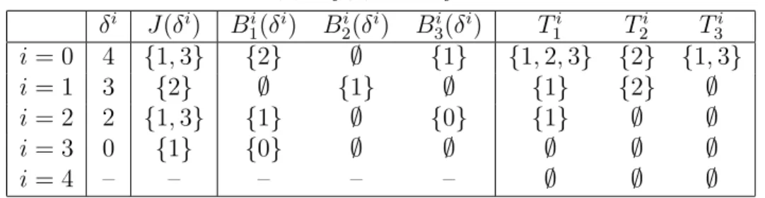
Table 1 shows δ, J (δ), Bj(δ) and Tj in Example 3.4 in the ith iteration of EEM for the identity of (3.2). For G1 ∈ Γ(G0, P ), we choose δ1 = 3∈∪j=13 (Fj+ G1j + G1j)\ (F ∪ ∪3 j=1T 1 j) ={0, 3}. Then we obtain J (δ1) and B1
For G2 ∈ Γ(G0, P ), we choose δ2 = 2∈∪3
j=1(Fj+ G2j + G2j)\ (F ∪ ∪3
j=1Tj2) ={0, 2}. Then we obtain J (δ2) and B2
j(δ2) in the fourth row of Table 1 and G3 = ({0}, {0}, ∅). This implies that f3 is redundant for all SOS representations of f with f1, f2, f3 and G3.
For G3 ∈ Γ(G0, P ), we choose δ3 = 0 ∈ ∪3
j=1(Fj + G3j + G3j)\ (F ∪ ∪3
j=1Tj3) = {0}. Then we obtain J (δ3) and B3
j(δ3) in the fifth row of Table 1 and G4 = (∅, {0}, ∅). This implies that f1 is redundant for all SOS representations of f with f1, f2, f3 and G4.
For G4 ∈ Γ(G0, P ), because the set∪3
j=1(Fj+ G 4 j+ G4j)\(F ∪ ∪3 j=1T 4 j) is empty, EEM stops and returns G∗ = (∅, {0}, ∅). Then by using G∗, from SOS problem (3.2), we obtain the following Linear Programming (LP):
{
Find λ2 ≥ 0
subjecto to λ2 = 1.
Because this LP has the solution λ2 = 1, SOS problem (3.2) has a solution (σ1, σ2, σ3) =
(0, 1, 0). This implies that f = 0· f1+ 1· f2+ 0· f3.
Table 1: δ, J (δ), Bj(δ) and Tj in Example 3.4
δi J (δi) B1i(δi) B2i(δi) B3i(δi) T1i T2i T3i i = 0 4 {1, 3} {2} ∅ {1} {1, 2, 3} {2} {1, 3} i = 1 3 {2} ∅ {1} ∅ {1} {2} ∅ i = 2 2 {1, 3} {1} ∅ {0} {1} ∅ ∅ i = 3 0 {1} {0} ∅ ∅ ∅ ∅ ∅ i = 4 – – – – – ∅ ∅ ∅
4. Numerical Results for Some POPs
In this section, we present the numerical performance of EEM for Lasserre’s and sparse SDP relaxations for Polynomial Optimization Problems (POPs) in [6] and randomly gen-erated POPs with a sparse structure. To this end, we explain how to apply EEM to SDP relaxations for POPs.
For given polynomials f , f1, . . . , fm, POP is formulated as follows: inf
x∈Rn{f(x) | fj(x)≥ 0 (j = 1, . . . , m)} . (4.1) We can reformulate POP (4.1) into the following problem:
sup
ρ∈R{ρ | f(x) − ρ ≥ 0 (∀x ∈ D)} .
(4.2)
Here D is the feasible region of POP (4.1). We choose an integer r with r ≥ ¯r. For (4.2) and r, we consider the following SOS problem:
ρ∗r := sup ρ∈R,σj∈Σrj { ρ f (x)− ρ = σ0+ m ∑ j=1 σj(x)fj(x) (∀x ∈ Rn) } (4.3)
where we define rj = r− ⌈deg(fj)/2⌉ for all j = 1, . . . , m and r0 = r. If we find a feasible
solution (ρ, σ0, σ1, . . . , σm) of (4.3), then ρ is a lower bound of optimal value of (4.1), clearly. It follows that ρ∗r+1 ≥ ρ∗r for all r ≥ ¯r because we have Σk ⊆ Σk+1 for all k ∈ N.
We apply EEM to the identity in (4.3). Then, we can regard f (x)− ρ in (4.3) as a polynomial with variable x. It should be noted that the support F of f (x)− ρ always contains 0 because−ρ is regarded as a constant term in the identity in (4.3). Moreover, let
f0(x) = 1 for all x∈ Rn. We replace σ0(x) by σ0(x)f0(x) in the identity in (4.3). Then we
can apply EEM directly, so that we obtain finite sets G∗0, G∗1, . . . , G∗m. We can construct an SDP problem by using G∗0, G∗1, . . . , G∗m and applying a similar argument described in subsection 2.1.
It was proposed in [20] to construct a smaller SDP relaxation problem than Lasserre’s SDP relaxation when a given POP has a special sparse structure called correlative sparsity. We call their method the WKKM sparse SDP relaxation for POPs in this paper. In the numerical experiments, we have tested EEM applied to both Lasserre’s and the WKKM sparse SDP relaxations.
We use a computer with Intel (R) Xeon (R) 2.40 GHz cpus and 24GB memory, and Matlab R2009b and SeDuMi 1.21 with the default parameters to solve the resulting SDP relaxation problems. In particular, the default tolerance for stopping criterion of SeDuMi is 1.0e-9. We use SparsePOP [21] to make SDP relaxation problems. To see the quality of the approximate solution obtained by SeDuMi, we check DIMACS errors. If the six errors are sufficiently small, then the solution is regarded as an optimal solution. See [10] for the definitions.
To check whether the optimal value of an SDP relaxation problem is the exact optimal value of a given POP or not, we use the following two criteria ϵobj and ϵfeas: Let ˆx be a candidate of an optimal solution of the POP obtained by Lasserre’s or the WKKM sparse SDP relaxation. See [20] for the way to obtain ˆx. We define:
ϵobj := |the optimal value of the SDP relaxation − f(ˆx)|max{1, f(ˆx)} , ϵfeas := min{fk(ˆx) (k = 1, . . . , m)}.
If ϵfeas = 0, then ˆx is feasible for the POP. In addition, if ϵobj = 0, then ˆx is an optimal solution of the POP and f (ˆx) is the optimal value of the POP.
Some POPs in [6] are so badly scaled that the resulting SDP relaxation problems suffer severe numerical difficulty. We may obtain inaccurate values and solutions for such POPs. To avoid this difficulty, we apply a linear transformation to the variables in POP with finite lower and upper bounds on variables xi (i = 1, . . . , n). See [24] for the effect of such transformations.
Although EMSSOSP is designed for an unconstrained POP, we can apply it to POP (4.1) in such a way that it removes unnecessary monomials in σ0 in (4.3). It is presented
in subsection 6.3 of [20] that such application of EMSSOSP is effective for a large-scale POP. In this section, we also compare EEM with EMSSOSP.
Table 2 shows notation used in the description of the numerical results in subsec-tions 4.1 and 4.2.
Table 2: Notation
Method a method for reducing the size of the SDP relaxation problems. “Orig.” means that we do not apply EMSSOSP and EEM to POPs. “EMSSOSP” and “EEM” mean that we apply EMSSOSP and EEM to POPs, respectively.
sizeA the size of coefficient matrix A in the SeDuMi input format
nnzA the number of nonzero elements in coefficient matrix A in the SeDuMi input format
#LP the number of linear constraints in the SeDuMi input format
#SDP the number of positive semidefinite constraints in the SeDuMi input format
a.SDP the average of the sizes of positive semidefinite constraints in the Se-DuMi input format
m.SDP the maximum of the sizes of positive semidefinite constraints in the SeDuMi input format
SDPobj the objective value obtained by SeDuMi for the resulting SDP relax-ation problem
POPobj the value of f at a solution ˆx retrieved by SparesPOP
eTime cpu time consumed by SeDuMi or SDPA-GMP in seconds
n.e. n.e. = 1 if SeDuMi cannot find an accurate solution due to numerical difficulty. Otherwise, n.e. = 0
p.v. phase value returned by GMP. If it is “pdOPT”, then SDPA-GMP terminates normally.
4.1. Numerical results for GLOBAL Library
In this numerical experiment, we solve some POPs in GLOBAL Library [6]. This library contains POPs which have polynomial equalities h(x) = 0. In this case, we divide h(x) = 0 into two polynomial inequalities h(x) ≥ 0 and −h(x) ≥ 0 and replace them by their polynomial inequalities in the original POP. We remark that in our tables, a POP whose initial is “B” is obtained by adding some lower and upper bounds. In addition, we do not apply the WKKM sparse SDP relaxation to POPs “Bex3 1 4”, “st e01”, “st e09” and “st e34” because their POPs do not have the sparse structure.
Tables 3 and 4 show the numerical results for Lasserre’s SDP relaxation [9] for some POPs in [6]. Tables 5 and 6 show the numerical results for the WKKM sparse SDP relaxation [20] for some POPs in [6].
We observe the following.
• From Tables 4 and 6, the sizes of SDP relaxation problems obtained by EEM are the
smallest of the three for all POPs. As a result, EEM spends the least cpu time to solve the resulting SDP problems except for Bst 07 on Table 3 and Bex 5 2 2 case2 on Table 5. Table 4 tells us that EEM needs one more iteration than that by EMSSOSP for Bst 07. Looking at the behavior of SeDuMi in this case carefully, we noticed that SeDuMi consumes much more CPU time in the last iteration for computing the search direction than in the other iterations. Also in the case of Bex 5 2 2 case2, EEM needs three more iterations than that by EMSSOSP. Exact reasons of them should be investigated in further research.
• For all POPs except for Bex5 2 2 case1, 2, 3, the optimal values of the SDP relaxation
problems are the same. For the WKKM sparse SDP relaxation of Bex5 2 2 case1, 2, 3, all three methods cannot obtain accurate solutions; their DIMACS errors are not sufficiently small. Consequently, these computed optimal values are considered to be inaccurate.
• From Tables 4 and 6, for almost all POPs, DIMACS errors for SDP relaxation problems
obtained by EEM are smaller than the other methods. This means that SeDuMi returns more accurate solutions for the resulting SDP relaxation problems by EEM.
• We cannot obtain optimal values and solutions for some POPs, e.g., Bex5 2 2 case1,
2, 3. In contrast, the optimal values and solutions for them are obtained in [20]. At a glance, it seems that the numerical result for some POPs may be worse than [20]. The reason is as follows: In [20], the authors add some valid polynomial inequalities to POPs and apply Lasserre’s or the WKKM sparse SDP relaxation, so that they obtain tighter lower bounds or the exact values. See Section 5.5 in [20] for the details. In the experiments of this section, however, we do not add such valid polynomial inequalities in order to observe the efficiency of EMSSOSP and EEM.
T able 3: Numerical results of Lasserre’s SDP relaxation problems Problem r Metho d SDP ob j POP ob j ϵ ob j ϵ feas ϵ ′ feas eTime Bex3 1 1 3 Orig. 7.049248e+03 7.049248e+03 2.5e-11 -3.662e-04 -1.812e-10 157.40 Bex3 1 1 3 EMSSOSP 7.049248e+03 7.049248e+03 2.7e-11 -4.041e-04 -1.999e-10 44.35 Bex3 1 1 3 EEM 7.049248e+03 7.049248e+03 6.2e-12 -1.024e-04 -5.064e-11 20.22 Bex3 1 4 4 Orig. -4.000002e+00 -4.000002e+00 5.4e-10 -1.069e-03 -2.741e-05 0.56 Bex3 1 4 4 EMSSOSP -4.000000e+00 -4.000000e+00 3.7e-10 -2.207e+00 -9.194e-02 0.55 Bex3 1 4 4 EEM -4.000000e+00 -4.000000e+00 4.4e-09 -2.193e+00 -9.139e-02 0.42 Bex5 2 2 case1 2 Orig. -4.000001e+02 -4.000002e+02 3.8e-07 -4.901e-02 -4.791e-04 3.47 Bex5 2 2 case1 2 EMSSOSP -4.000001e+02 -4.000002e+02 2.2e-07 -3.743e-02 -3.663e-04 0.42 Bex5 2 2 case1 2 EEM -4.000001e+02 -4.000002e+02 2.2e-07 -3.743e-02 -3.663e-04 0.42 Bex5 2 2 case2 2 Orig. -6.000000e+02 -6.000001e+02 1.3e-07 -2.405e-02 -1.919e-04 3.35 Bex5 2 2 case2 2 EMSSOSP -6.000001e+02 -6.000002e+02 2.6e-07 -4.543e-02 -3.790e-04 0.44 Bex5 2 2 case2 2 EEM -6.000001e+02 -6.000002e+02 2.6e-07 -4.543e-02 -3.790e-04 0.44 Bex5 2 2 case3 2 Orig. -7.500000e+02 -7.500000e+02 9.8e-09 -4.246e-03 -1.415e-05 3.03 Bex5 2 2 case3 2 EMSSOSP -7.500000e+02 -7.500000e+02 1.2e-08 -2.391e-03 -7.968e-06 0.37 Bex5 2 2 case3 2 EEM -7.500000e+02 -7.500000e+02 1.2e-08 -2.391e-03 -7.968e-06 0.36 Bst e07 2 Orig. -1.809184e+03 -1.809184e+03 8.4e-12 -1.125e-05 -1.837e-08 4.91 Bst e07 2 EMSSOSP -1.809184e+03 -1.809184e+03 1.5e-11 -2.012e-05 -3.286e-08 0.64 Bst e07 2 EEM -1.809184e+03 -1.809184e+03 3.5e-12 -4.666e-06 -7.621e-09 0.75 Bst e33 2 Orig. -4.000000e+02 -4.000000e+02 8.6e-11 -3.178e-09 -1.254e-09 2.36 Bst e33 2 EMSSOSP -4.000000e+02 -4.000000e+02 1.6e-10 -7.255e-09 -2.812e-09 0.29 Bst e33 2 EEM -4.000000e+02 -4.000000e+02 1.6e-10 -7.255e-09 -2.812e-09 0.29 st e01 3 Orig. -6.666667e+00 -6.666667e+00 1.6e-11 -3.183e-09 -7.957e-10 0.06 st e01 3 EMSSOSP -6.666667e+00 -6.666667e+00 4.5e-12 -2.173e-10 -5.433e-11 0.05 st e01 3 EEM -6.666667e+00 -6.666667e+00 5.3e-10 -8.596e-09 -2.149e-09 0.04 st e09 3 Orig. -5.000000e-01 -5.000000e-01 2.8e-10 0.000e+00 0.000e+00 0.05 st e09 3 EMSSOSP -5.000000e-01 -5.000000e-01 8.8e-10 0.000e+00 0.000e+00 0.05 st e09 3 EEM -5.000000e-01 -5.000000e-01 9.3e-10 0.000e+00 0.000e+00 0.04 st e34 2 Orig. 1.561953e-02 1.561953e-02 2.3e-10 0.000e+00 0.000e+00 0.32 st e34 2 EMSSOSP 1.561953e-02 1.561953e-02 6.6e-11 0.000e+00 0.000e+00 0.32 st e34 2 EEM 1.561952e-02 1.561952e-02 6.3e-12 -1.968e-06 -3.960e-07 0.16
T able 4: Numerical errors, iterations, DIMA CS errors and sizes of Lasserre’s SDP relaxation problems. W e omit err2 and err3 from this table b ecause they are zero for all POPs and metho ds. Problem r Metho d n.e. iter. err1 err4 err5 err6 sizeA nnzA #LP #SDP a.SDP m.SDP Bex3 1 1 3 Orig. 0 20 2.4e-09 6.0e-12 -1.2e-11 5.8e-09 3002 × 71775 126436 0 23 50.22 165 Bex3 1 1 3 EMSSOSP 0 20 2.6e-09 6.4e-12 -1.3e-11 5.1e-09 2171 × 51439 104840 0 23 46.65 83 Bex3 1 1 3 EEM 0 21 6.5e-10 1.6e-12 -2.9e-12 7.0e-10 1286 × 40743 72076 0 23 40.30 45 Bex3 1 4 4 Orig. 0 18 1.5e-10 1.8e-11 -1.8e-10 1.4e-10 164 × 4825 11618 0 10 21.50 35 Bex3 1 4 4 EMSSOSP 0 18 2.0e-10 1.7e-11 -1.2e-10 3.3e-10 164 × 4825 11618 0 10 21.50 35 Bex3 1 4 4 EEM 0 18 6.7e-11 6.1e-11 -1.5e-09 -1.4e-09 119 × 3700 7793 0 10 19.00 20 Bex5 2 2 case1 2 Orig. 0 21 2.7e-10 2.5e-11 -2.7e-08 -1.8e-08 714 × 5245 7085 0 21 12.14 55 Bex5 2 2 case1 2 EMSSOSP 0 19 6.7e-10 2.0e-11 -1.6e-08 -1.5e-08 300 × 2364 4204 0 21 10.10 12 Bex5 2 2 case1 2 EEM 0 19 6.7e-10 2.0e-11 -1.6e-08 -1.5e-08 300 × 2364 4204 0 21 10.10 12 Bex5 2 2 case2 2 Orig. 0 21 4.3e-11 4.7e-12 -8.2e-09 -6.4e-09 714 × 5245 7085 0 21 12.14 55 Bex5 2 2 case2 2 EMSSOSP 0 20 2.4e-11 8.8e-12 -1.7e-08 -1.7e-08 300 × 2364 4204 0 21 10.10 12 Bex5 2 2 case2 2 EEM 0 20 2.4e-11 8.8e-12 -1.7e-08 -1.7e-08 300 × 2364 4204 0 21 10.10 12 Bex5 2 2 case3 2 Orig. 0 18 1.6e-10 1.4e-11 -1.4e-09 5.8e-10 714 × 5245 7085 0 21 12.14 55 Bex5 2 2 case3 2 EMSSOSP 0 16 6.1e-11 8.2e-12 -1.7e-09 -1.6e-09 300 × 2364 4204 0 21 10.10 12 Bex5 2 2 case3 2 EEM 0 16 6.1e-11 8.2e-12 -1.7e-09 -1.6e-09 300 × 2364 4204 0 21 10.10 12 Bst e07 2 Orig. 0 17 1.1e-10 2.4e-13 -1.8e-12 4.1e-10 1000 × 7348 10131 0 23 13.39 66 Bst e07 2 EMSSOSP 0 16 2.4e-10 7.6e-13 -3.3e-12 5.4e-10 430 × 3188 5971 0 23 11.13 14 Bst e07 2 EEM 0 17 5.5e-11 1.7e-13 -7.4e-13 1.1e-10 385 × 3044 5476 0 23 10.70 13 Bst e33 2 Orig. 0 14 2.2e-10 6.5e-13 -6.1e-12 1.0e-09 714 × 5245 7395 0 21 12.14 55 Bst e33 2 EMSSOSP 0 12 4.5e-10 1.4e-12 -1.1e-11 1.2e-09 300 × 2364 4514 0 21 10.10 12 Bst e33 2 EEM 0 12 4.5e-10 1.4e-12 -1.1e-11 1.2e-09 300 × 2364 4514 0 21 10.10 12 st e01 3 Orig. 0 11 8.6e-11 2.4e-12 -5.5e-12 1.3e-10 27 × 280 384 0 6 6.67 10 st e01 3 EMSSOSP 0 11 3.3e-11 5.0e-13 -1.6e-12 3.8e-11 25 × 244 348 0 6 6.33 8 st e01 3 EEM 0 9 2.6e-10 8.0e-12 1.8e-10 3.8e-10 20 × 189 266 0 6 5.50 6 st e09 3 Orig. 0 11 2.2e-10 5.9e-12 1.6e-10 3.5e-10 27 × 280 456 0 6 6.67 10 st e09 3 EMSSOSP 0 10 3.0e-10 2.0e-11 4.1e-10 6.0e-10 25 × 244 420 0 6 6.33 8 st e09 3 EEM 0 9 3.0e-10 1.9e-11 4.0e-10 4.8e-10 20 × 189 284 0 6 5.50 6 st e34 2 Orig. 0 22 9.6e-11 5.9e-14 5.4e-11 1.1e-10 209 × 1568 3272 0 17 8.24 28 st e34 2 EMSSOSP 0 27 3.7e-12 1.0e-13 1.5e-11 2.8e-11 158 × 953 2639 0 17 7.35 13 st e34 2 EEM 0 22 2.3e-14 2.8e-14 1.4e-12 1.5e-12 83 × 641 953 4 13 7.00 7
T able 5: Numerical results of the WKKM sparse SDP relaxation problems Problem r Metho d SDP ob j POP ob j ϵ ob j ϵ feas ϵ ′ feas eTime Bex3 1 1 3 Orig. 7.049248e+03 7.049248e+03 1.8e-11 -3.137e-04 -1.552e-10 0.87 Bex3 1 1 3 EMSSOSP 7.049248e+03 7.049248e+03 2.1e-11 -3.819e-04 -1.889e-10 0.59 Bex3 1 1 3 EEM 7.049248e+03 7.049248e+03 2.4e-11 -4.335e-04 -2.144e-10 0.30 Bex5 2 2 case1 2 Orig. -4.778484e+02 -4.779311e+02 1.7e-04 -5.678e+02 -9.157e-01 0.71 Bex5 2 2 case1 2 EMSSOSP -4.778414e+02 -4.778925e+02 1.1e-04 -5.678e+02 -9.156e-01 0.37 Bex5 2 2 case1 2 EEM -4.778472e+02 -4.779112e+02 1.3e-04 -5.676e+02 -9.156e-01 0.35 Bex5 2 2 case1 3 Orig. -4.086439e+02 -4.100943e+02 3.5e-03 -3.737e+02 -8.124e-01 5.41 Bex5 2 2 case1 3 EMSSOSP -4.002579e+02 -4.002719e+02 3.5e-05 -3.535e+01 -2.465e-01 3.11 Bex5 2 2 case1 3 EEM -4.000032e+02 -4.000075e+02 1.1e-05 -6.845e-01 -6.340e-03 2.02 Bex5 2 2 case2 2 Orig. -8.499660e+02 -8.499680e+02 2.3e-06 -8.569e+02 -7.360e-01 1.05 Bex5 2 2 case2 2 EMSSOSP -8.498378e+02 -8.498394e+02 1.9e-06 -8.564e+02 -7.359e-01 0.37 Bex5 2 2 case2 2 EEM -8.498379e+02 -8.498395e+02 1.9e-06 -8.564e+02 -7.359e-01 0.36 Bex5 2 2 case2 3 Orig. -6.456600e+02 -6.841458e+02 6.0e-02 -2.015e+03 -8.918e-01 5.67 Bex5 2 2 case2 3 EMSSOSP -6.016427e+02 -6.021145e+02 7.8e-04 -4.235e+02 -7.415e-01 3.21 Bex5 2 2 case2 3 EEM -6.001027e+02 -6.001363e+02 5.6e-05 -2.073e+01 -5.488e-01 3.40 Bex5 2 2 case3 2 Orig. -7.695283e+02 -7.695349e+02 8.6e-06 -6.731e+01 -2.204e-01 0.75 Bex5 2 2 case3 2 EMSSOSP -7.695063e+02 -7.695068e+02 6.8e-07 -6.696e+01 -2.194e-01 0.45 Bex5 2 2 case3 2 EEM -7.695067e+02 -7.695072e+02 6.9e-07 -6.688e+01 -2.192e-01 0.40 Bex5 2 2 case3 3 Orig. -7.503488e+02 -7.504064e+02 7.7e-05 -1.715e+01 -5.430e-02 6.24 Bex5 2 2 case3 3 EMSSOSP -7.500063e+02 -7.500092e+02 3.8e-06 -1.670e+00 -5.539e-03 3.04 Bex5 2 2 case3 3 EEM -7.500001e+02 -7.500001e+02 3.7e-09 -1.204e-02 -4.013e-05 2.20 Bst e07 2 Orig. -1.809184e+03 -1.809184e+03 9.6e-12 -1.409e-05 -2.302e-08 0.50 Bst e07 2 EMSSOSP -1.809184e+03 -1.809184e+03 5.6e-10 -7.653e-06 -1.250e-08 0.19 Bst e07 2 EEM -1.809184e+03 -1.809184e+03 5.8e-10 -1.079e-05 -1.762e-08 0.17 Bst e33 2 Orig. -4.000000e+02 -4.000000e+02 1.1e-09 -4.381e-09 -2.190e-09 0.30 Bst e33 2 EMSSOSP -4.000000e+02 -4.000000e+02 5.7e-10 -1.026e-09 -5.132e-10 0.13 Bst e33 2 EEM -4.000000e+02 -4.000000e+02 8.6e-10 -1.257e-09 -6.285e-10 0.11
T able 6: Numerical errors, iterations, DIMA CS errors and sizes of the WKKM sparse SDP relaxation problems. W e omit err2 and err3 from this table b ecause they are zero for all POPs and metho ds. Problem r Metho d n.e. iter. err1 err4 err5 err6 sizeA nnzA #LP #SDP a.SDP m.SDP Bex3 1 1 3 Orig. 0 16 8.3e-10 2.8e-12 -8.6e-12 1.5e-09 363 × 4975 8784 0 25 13.00 35 Bex3 1 1 3 EMSSOSP 0 16 1.0e-09 3.4e-12 -1.0e-11 1.5e-09 295 × 3828 7589 0 25 12.00 22 Bex3 1 1 3 EEM 0 16 1.2e-09 3.8e-12 -1.1e-11 1.0e-09 225 × 3007 5344 0 25 10.52 15 Bex5 2 2 case1 2 Orig. 0 40 4.2e-11 4.4e-11 -1.4e-05 -1.3e-05 235 × 1507 2028 0 23 6.74 21 Bex5 2 2 case1 2 EMSSOSP 0 38 3.9e-11 2.9e-11 -8.9e-06 -8.8e-06 137 × 752 1264 0 23 5.39 8 Bex5 2 2 case1 2 EEM 0 38 3.6e-11 3.6e-11 -1.1e-05 -1.1e-05 123 × 720 1168 0 23 5.22 8 Bex5 2 2 case1 3 Orig. 1 27 3.4e-07 3.0e-08 -2.6e-04 7.0e-04 825 × 11342 15723 0 23 19.57 56 Bex5 2 2 case1 3 EMSSOSP 1 33 7.1e-09 1.8e-09 -2.5e-06 2.2e-05 603 × 7378 11727 0 23 17.04 30 Bex5 2 2 case1 3 EEM 0 34 4.0e-11 3.8e-11 -7.7e-07 -7.5e-07 543 × 6912 10617 0 23 16.26 30 Bex5 2 2 case2 2 Orig. 0 39 2.4e-10 4.6e-11 -2.1e-07 9.4e-06 235 × 1507 2028 0 23 6.74 21 Bex5 2 2 case2 2 EMSSOSP 0 37 5.2e-11 2.5e-11 -1.7e-07 5.1e-07 137 × 752 1264 0 23 5.39 8 Bex5 2 2 case2 2 EEM 0 37 5.1e-11 2.5e-11 -1.7e-07 -1.7e-07 123 × 720 1168 0 23 5.22 8 Bex5 2 2 case2 3 Orig. 1 30 2.6e-07 2.9e-08 -4.1e-03 -3.2e-03 825 × 11342 15723 0 23 19.57 56 Bex5 2 2 case2 3 EMSSOSP 1 36 1.8e-08 1.9e-09 -5.1e-05 3.2e-05 603 × 7378 11727 0 23 17.04 30 Bex5 2 2 case2 3 EEM 1 39 9.2e-10 9.4e-11 -3.6e-06 -2.7e-06 543 × 6912 10617 0 23 16.26 30 Bex5 2 2 case3 2 Orig. 0 41 1.3e-10 4.2e-11 -1.2e-06 1.3e-06 235 × 1507 2028 0 23 6.74 21 Bex5 2 2 case3 2 EMSSOSP 0 38 9.8e-11 9.4e-12 -9.6e-08 -1.7e-08 137 × 752 1264 0 23 5.39 8 Bex5 2 2 case3 2 EEM 0 36 9.6e-11 1.0e-11 -9.7e-08 -9.7e-08 123 × 720 1168 0 23 5.22 8 Bex5 2 2 case3 3 Orig. 1 30 5.2e-08 8.3e-09 -1.1e-05 2.6e-05 825 × 11342 15723 0 23 19.57 56 Bex5 2 2 case3 3 EMSSOSP 1 34 2.0e-09 4.6e-10 -5.3e-07 4.0e-07 603 × 7378 11727 0 23 17.04 30 Bex5 2 2 case3 3 EEM 0 35 2.9e-11 3.3e-12 -5.1e-10 7.4e-10 543 × 6912 10617 0 23 16.26 30 Bst e07 2 Orig. 0 20 1.5e-10 2.9e-13 -2.1e-12 5.2e-10 296 × 2209 2888 0 28 7.61 21 Bst e07 2 EMSSOSP 0 16 3.5e-11 4.0e-13 1.2e-10 1.8e-10 171 × 1037 1707 0 28 5.75 9 Bst e07 2 EEM 0 16 4.6e-11 5.2e-13 1.3e-10 1.8e-10 154 × 954 1504 1 27 5.59 8 Bst e33 2 Orig. 0 21 7.7e-11 3.2e-13 7.7e-11 3.9e-10 235 × 1507 2120 0 23 6.74 21 Bst e33 2 EMSSOSP 0 15 2.7e-11 7.4e-14 4.1e-11 9.4e-11 137 × 752 1356 0 23 5.39 8 Bst e33 2 EEM 0 15 1.5e-11 1.0e-13 6.1e-11 8.8e-11 123 × 720 1228 0 23 5.22 8
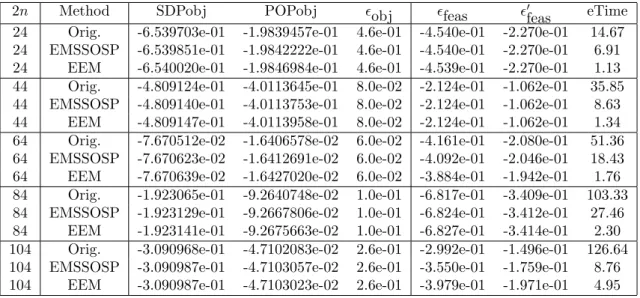
Table 7: Numerical results of the WKKM sparse SDP relaxation problems with relaxation order r = 2 for POP (4.4)
2n Method SDPobj POPobj ϵobj ϵfeas ϵ′feas eTime
24 Orig. -6.539703e-01 -1.9839457e-01 4.6e-01 -4.540e-01 -2.270e-01 14.67
24 EMSSOSP -6.539851e-01 -1.9842222e-01 4.6e-01 -4.540e-01 -2.270e-01 6.91
24 EEM -6.540020e-01 -1.9846984e-01 4.6e-01 -4.539e-01 -2.270e-01 1.13
44 Orig. -4.809124e-01 -4.0113645e-01 8.0e-02 -2.124e-01 -1.062e-01 35.85
44 EMSSOSP -4.809140e-01 -4.0113753e-01 8.0e-02 -2.124e-01 -1.062e-01 8.63
44 EEM -4.809147e-01 -4.0113958e-01 8.0e-02 -2.124e-01 -1.062e-01 1.34
64 Orig. -7.670512e-02 -1.6406578e-02 6.0e-02 -4.161e-01 -2.080e-01 51.36
64 EMSSOSP -7.670623e-02 -1.6412691e-02 6.0e-02 -4.092e-01 -2.046e-01 18.43
64 EEM -7.670639e-02 -1.6427020e-02 6.0e-02 -3.884e-01 -1.942e-01 1.76
84 Orig. -1.923065e-01 -9.2640748e-02 1.0e-01 -6.817e-01 -3.409e-01 103.33
84 EMSSOSP -1.923129e-01 -9.2667806e-02 1.0e-01 -6.824e-01 -3.412e-01 27.46
84 EEM -1.923141e-01 -9.2675663e-02 1.0e-01 -6.827e-01 -3.414e-01 2.30
104 Orig. -3.090968e-01 -4.7102083e-02 2.6e-01 -2.992e-01 -1.496e-01 126.64
104 EMSSOSP -3.090987e-01 -4.7103057e-02 2.6e-01 -3.550e-01 -1.759e-01 8.76
104 EEM -3.090987e-01 -4.7103023e-02 2.6e-01 -3.979e-01 -1.971e-01 4.95
4.2. Numerical results for randomly generated POP with a special structure
Let Ci = {i, i + 1, i + 2} for all i = 1, . . . , n − 2. xCi and yCi denote the subvec-tors (xi, xi+1, xi+2) and (yi, yi+1, yi+2) of x, y∈ Rn, respectively. We consider the following POP: infx,y∈Rn n−2 ∑ i=1 (xCi, yCi) T Pi ( xCi yCi ) subject to xT CiQiyCi + c T i xCi+ d T i yCi+ γi ≥ 0 (i = 1, . . . , n − 2), 0≤ xi, yi ≤ 1 (i = 1, . . . , n), (4.4)
where ci, di ∈ R3, Qi ∈ R3×3, and Pi ∈ S6×6 is a symmetric positive semidefinite matrix. This POP has 2n variables and 5n− 2 polynomial inequalities.
In this subsection, we generate POP (4.4) randomly and apply the WKKM sparse SDP relaxation with relaxation order r = 2, 3. The SDP relaxation problems obtained by Lasserre’s SDP relaxation are too large-scale to be handled for these problems.
Tables 7 and 8 show the numerical results of the WKKM sparse SDP relaxation with relaxation order r = 2. To obtain more accurate values and solutions, we use SDPA-GMP [5]. Tables 11 and 12 show the numerical result by SDPA-SDPA-GMP with tolerance
ϵ = 1.0e-15 and precision 256. With this precision, SDPA-GMP calculate floating point
numbers with approximately 77 significant digits. Tables 9 and 10 show the numerical results of the WKKM sparse SDP relaxation with relaxation order r = 3. Tables 13 and 14 show the numerical result by SDPA-GMP with the same tolerance and precision as above. In this case, we solve only 2n = 24 and 44 because otherwise the resulting SDP problems become too large-scale to be solved by SDPA-GMP.
T able 8: Numerical errors, iterations, DIMA CS errors and sizes of the WKKM sparse SDP relaxation problems with relaxation order r = 2 for POP (4.4). W e omit err2 and err3 from this table b ecause they are zero for all POPs and metho ds. 2 n Metho d n.e. iter. err1 err4 err5 err6 sizeA nnzA #LP #SDP a.SDP m.SDP 24 Orig. 1 49 2.1e-09 0.0e+00 -1.9e-08 1.6e-05 2015 × 16192 26728 0 69 11.88 36 24 EMSSOSP 1 51 2.4e-09 0.0e+00 -1.0e-08 6.9e-06 1101 × 6572 15050 0 69 9.16 19 24 EEM 0 20 1.4e-10 6.6e-13 5.6e-10 1.2e-09 593 × 3531 5067 10 59 7.71 8 44 Orig. 0 59 2.7e-10 0.0e+00 -8.8e-08 1.4e-06 4055 × 32352 53728 0 129 12.25 36 44 EMSSOSP 0 55 1.7e-10 0.0e+00 -3.5e-10 3.7e-07 2201 × 12662 29745 0 129 9.32 19 44 EEM 0 21 9.3e-11 7.8e-13 7.9e-10 1.4e-09 1233 × 6741 9667 20 109 7.84 8 64 Orig. 1 58 5.5e-09 0.0e+00 -3.8e-08 1.6e-06 6095 × 48512 80728 0 189 12.38 36 64 EMSSOSP 1 53 2.7e-09 0.0e+00 -9.0e-11 1.9e-07 3301 × 18752 44457 0 189 9.38 19 64 EEM 0 27 9.1e-12 6.1e-15 4.2e-11 9.9e-11 1873 × 9951 14267 30 159 7.89 8 84 Orig. 1 64 8.1e-09 0.0e+00 -2.8e-09 9.5e-06 7940 × 62821 105067 0 249 12.27 36 84 EMSSOSP 1 63 6.9e-10 0.0e+00 -1.5e-07 8.6e-07 4332 × 24428 58239 0 249 9.31 19 84 EEM 0 20 3.7e-11 5.7e-14 1.0e-10 2.5e-10 2465 × 12846 18417 40 209 7.82 8 104 Orig. 0 88 3.7e-10 0.0e+00 -1.7e-07 1.6e-06 9916 × 78394 131225 0 309 12.30 36 104 EMSSOSP 0 25 6.1e-11 9.8e-14 5.6e-10 1.2e-09 5410 × 30410 72723 0 309 9.33 19 104 EEM 0 22 1.8e-10 2.2e-15 1.3e-10 9.7e-10 3090 × 15981 22912 50 259 7.83 8
T able 9: Numerical results of the WKKM sparse SDP relaxation problems with relaxation order r = 3 for POP (4.4) 2 n Metho d SDP ob j POP ob j ϵ ob j ϵ feas ϵ ′ feas eTime 24 Orig. -5.160104e-01 -5.1400753e-01 2.0e-03 0.000e+00 0.000e+00 475.04 24 EMSSOSP -5.160105e-01 -5.1400132e-01 2.0e-03 0.000e+00 0.000e+00 190.01 24 EEM -5.160105e-01 -5.1401615e-01 2.0e-03 0.000e+00 0.000e+00 35.51 44 Orig. -4.409558e-01 -4.2159001e-01 1.9e-02 -5.408e-02 -2.704e-02 1650.50 44 EMSSOSP -4.409530e-01 -4.2158583e-01 1.9e-02 -5.704e-02 -2.852e-02 338.54 44 EEM -4.409561e-01 -4.2158866e-01 1.9e-02 -5.894e-02 -2.947e-02 98.19 64 Orig. -6.235235e-02 -6.2352342e-02 6.3e-09 -1.208e-01 -6.039e-02 1316.66 64 EMSSOSP -6.235225e-02 -6.2352050e-02 2.0e-07 -1.265e-01 -6.327e-02 551.48 64 EEM -6.235235e-02 -6.2352349e-02 1.4e-09 -1.219e-01 -6.095e-02 114.98 84 Orig. -1.344148e-01 -1.0153127e-01 3.3e-02 -8.336e-02 -4.168e-02 2321.02 84 EMSSOSP -1.344157e-01 -1.0148873e-01 3.3e-02 -8.324e-02 -4.162e-02 962.95 84 EEM -1.344151e-01 -1.0153038e-01 3.3e-02 -8.340e-02 -4.170e-02 256.85 104 Orig. -1.579301e-01 -8.8999964e-02 6.9e-02 -2.032e-01 -1.016e-01 2956.81 104 EMSSOSP -1.578784e-01 -8.8947707e-02 6.9e-02 -2.101e-01 -1.050e-01 744.44 104 EEM -1.579325e-01 -8.8995970e-02 6.9e-02 -2.171e-01 -1.086e-01 279.25 T able 10: Numerical errors, iterations, DIMA CS errors and sizes of the sparse SDP relaxation problems with relaxation order r = 3 for POP (4.4). W e omit err2 and err3 from this table b ecause they are zero for all POPs and metho ds. 2 n Metho d n.e. iter. err1 err4 err5 err6 sizeA nnzA #LP #SDP a.SDP m.SDP 24 Orig. 1 39 2.7e-09 3.3e-12 -3.3e-11 1.0e-07 11995 × 203344 409859 0 69 45.97 120 24 EMSSOSP 1 33 8.1e-09 1.1e-11 -6.6e-11 1.6e-07 9283 × 131628 325901 0 69 40.52 86 24 EEM 1 31 1.5e-09 2.0e-12 -1.1e-11 1.7e-08 4770 × 68370 104995 0 69 29.94 36 44 Orig. 1 54 1.3e-08 7.0e-12 -8.1e-11 4.8e-07 24535 × 412144 838939 0 129 47.84 120 44 EMSSOSP 1 29 3.5e-07 2.0e-10 -1.4e-09 6.6e-06 18940 × 262038 662594 0 129 41.91 86 44 EEM 1 35 6.4e-09 3.5e-12 -2.1e-11 6.8e-08 10170 × 133810 205915 0 129 30.59 36 64 Orig. 1 36 9.5e-10 1.2e-13 -1.4e-12 1.4e-08 37075 × 620944 1268019 0 189 48.53 120 64 EMSSOSP 1 31 3.8e-08 7.1e-12 -5.1e-11 4.2e-07 28594 × 392448 999618 0 189 42.41 86 64 EEM 0 33 2.5e-10 4.8e-14 -3.1e-13 2.0e-09 15570 × 199250 306835 0 189 30.83 36 84 Orig. 1 46 3.8e-08 5.0e-12 -5.8e-09 1.1e-06 47964 × 796960 1636667 0 249 47.78 120 84 EMSSOSP 1 42 7.1e-07 1.0e-10 1.1e-06 8.9e-06 37121 × 504711 1293315 0 249 41.80 86 84 EEM 1 38 1.6e-09 2.8e-12 -4.0e-12 1.2e-08 20327 × 253893 391675 0 249 30.26 36 104 Orig. 1 44 1.2e-07 6.3e-12 -2.9e-10 4.5e-06 59964 × 995856 2047139 0 309 47.96 120 104 EMSSOSP 1 26 1.6e-05 8.0e-10 -1.7e-08 2.5e-04 46408 × 630096 1617625 0 309 41.94 86 104 EEM 1 36 1.8e-09 8.7e-14 -1.7e-12 1.6e-08 25523 × 316758 488771 0 309 30.34 36
Table 11: Numerical results by SDPA-GMP 7.1.2 with ϵ=1.0e-15 for the WKKM sparse SDP relaxation problems with relaxation order r = 2 in POP (4.4)
2n Method p.v. iter. eTime SDPobj by SDPA-GMP SDPobj by SeDuMi
24 Orig. pdOPT 53 719.260 -6.54001981e-01 -6.539703e-01
24 EMSSOSP pdOPT 49 115.920 -6.54001981e-01 -6.539851e-01
24 EEM pdOPT 44 17.370 -6.54001981e-01 -6.540020e-01
44 Orig. pdOPT 57 1655.640 -4.80914669e-01 -4.809124e-01
44 EMSSOSP pdOPT 50 249.480 -4.80914669e-01 -4.809140e-01
44 EEM pdOPT 43 31.350 -4.80914669e-01 -4.809147e-01
64 Orig. pdOPT 58 2599.260 -7.67063944e-02 -7.670512e-02
64 EMSSOSP pdOPT 52 385.260 -7.67063944e-02 -7.670623e-02
64 EEM pdOPT 48 53.090 -7.67063944e-02 -7.670639e-02
84 Orig. pdOPT 53 3066.100 -1.92314133e-01 -1.923065e-01
84 EMSSOSP pdOPT 48 453.890 -1.92314133e-01 -1.923129e-01
84 EEM pdOPT 41 60.660 -1.92314133e-01 -1.923141e-01
104 Orig. pdOPT 59 4341.780 -3.09098714e-01 -3.090968e-01
104 EMSSOSP pdOPT 50 625.520 -3.09098714e-01 -3.090987e-01
104 EEM pdOPT 46 80.070 -3.09098714e-01 -3.090987e-01
Table 12: DIMACS errors by SDPA-GMP 7.1.2 with ϵ=1.0e-15 for the sparse SDP relax-ation problems with relaxrelax-ation order r = 2 in POP (4.4). We omit err2 and err4 from this table because they are zero for all POPs and methods.
2n Method err1 err3 err5 err6
24 Orig. 2.987e-32 7.456e-74 2.595e-16 3.272e-16
24 EMSSOSP 2.013e-33 3.365e-74 3.473e-16 3.729e-16
24 EEM 1.682e-68 3.950e-77 3.877e-16 3.877e-16
44 Orig. 1.852e-31 1.059e-73 3.274e-16 4.486e-16
44 EMSSOSP 1.549e-32 7.730e-74 3.861e-16 4.448e-16
44 EEM 2.012e-68 2.908e-77 7.564e-17 7.564e-17
64 Orig. 4.578e-31 8.935e-74 6.357e-16 8.141e-16
64 EMSSOSP 7.600e-33 6.223e-74 6.360e-16 6.889e-16
64 EEM 2.402e-76 4.331e-77 3.539e-16 3.539e-16
84 Orig. 6.983e-32 2.500e-73 6.106e-16 9.097e-16
84 EMSSOSP 1.859e-34 9.731e-61 2.978e-16 3.202e-16
84 EEM 9.632e-69 4.153e-77 4.269e-16 4.269e-16
104 Orig. 3.615e-31 1.695e-73 4.399e-16 7.407e-16
104 EMSSOSP 8.722e-34 1.041e-73 1.602e-16 1.698e-16
104 EEM 1.798e-68 2.114e-77 1.703e-16 1.703e-16
We observe the following.
• The sizes of the resulting SDP relaxation problems by EEM is again the smallest in
the three methods. In particular, when we apply EEM and the WKKM sparse SDP relaxation with relaxation order r = 2, positive semidefinite constraints corresponding to the quadratic constraints in (4.2) are replaced by linear constraints in SDP relaxation problems. EEM removes all monomials except for the constant term in σj ∈ Σ1because
those monomials are redundant for all SOS representations of f . Then σj ∈ Σ1 for
all j = 1, . . . , n can be replaced by σj ∈ Σ0 for all j = 1, . . . , n. This is equivalent to
σj ≥ 0 for all j = 1, . . . , n. Therefore, we obtain n linear constraints in the resulting SDP relaxation problems.
Table 13: Numerical results by SDPA-GMP 7.1.2 with ϵ=1.0e-15 for the WKKM sparse SDP relaxation problems with relaxation order r = 3 in POP (4.4)
2n Method p.v. iter. eTime SDPobj by SDPA-GMP SDPobj by SeDuMi
24 Orig. pdOPT 63 108657.790 -5.16010521e-01 -5.160104e-01
24 EMSSOSP pdOPT 62 50558.410 -5.16010521e-01 -5.160105e-01
24 EEM pdOPT 60 5815.020 -5.16010521e-01 -5.160105e-01
44 Orig. pdOPT 71 268508.010 -4.40956190e-01 -4.409558e-01
44 EMSSOSP pdOPT 70 125076.640 -4.40956190e-01 -4.409530e-01
44 EEM pdOPT 67 13884.150 -4.40956190e-01 -4.409561e-01
Table 14: DIMACS errors by SDPA-GMP 7.1.2 with ϵ=1.0e-15 for the sparse SDP relax-ation problems with relaxrelax-ation order r = 3 in POP (4.4). We omit err2 and err4 from this table because they are zero for all POPs and methods.
2n Method err1 err3 err5 err6
24 Orig. 3.769e-30 1.713e-73 4.862e-16 5.763e-16
24 EMSSOSP 3.433e-30 2.059e-58 2.822e-16 3.196e-16
24 EEM 1.229e-65 3.354e-76 2.458e-16 2.458e-16
44 Orig. 6.368e-30 2.474e-73 3.905e-16 4.838e-16
44 EMSSOSP 5.010e-30 2.579e-73 4.820e-16 5.563e-16
44 EEM 4.523e-66 5.239e-76 3.112e-16 3.112e-16
• From Tables 11 and 12, SDPA-GMP with precision 256 can solve all SDP relaxation
problems accurately. In particular, SDPA-GMP solves SDP relaxation problems ob-tained by EEM more than 8 and 50 times faster than EMSSOSP and Orig., respectively.
• From Tables 7, 8 and 11, SeDuMi returns the optimal values of SDP relaxation
prob-lems obtained by EEM almost exactly as accurately as SDPA-GMP and more than 15 times faster than SDPA-GMP, while SeDuMi terminates before we obtain accurate solutions of SDP relaxation problems obtained by the other methods.
• From Table 10, in SDP relaxation problems with relaxation order r = 3, DIMACS
errors for SDP relaxation problems by EEM are the smallest in all methods. Moreover, from Tables 13 and 14, the optimal values of SDP relaxation problems by EEM coincide the optimal values found by SDPA-GMP for 2n = 24 and 44. However, SeDuMi cannot obtain accurate solutions because these values are larger than the tolerance 1.0e-9 of SeDuMi.
5. An Application of EEM to Specific POPs
As we have seen in Section 3, we have a flexibility in choosing δ although EEM always returns the smallest set G∗ ∈ Γ(G0, P ). We focus on this flexibility and we prove the
following two facts in this section: (i) if POP (4.1) satisfies a specific assumption, each optimal value of the SDP relaxation problem with relaxation order r > ¯r is equal to that
of the relaxation order ¯r. To prove this fact, we choose δ to be the largest element in
∪m
j=0(Fj+ Gj+ Gj)\ (F ∪ ∪m
j=0Tj) with the graded lexicographic order∗. (ii) We give an extension of Proposition 4 in [7], where we choose δ to be the smallest element.
∗We define the graded lexicographic order α⪰ β for α, β ∈ Nnas follows: |α| > |β| or , |α| = |β| and αi>
First of all, we state (i) exactly. Let γj be the largest element with the graded lexico-graphic order in Fj. For γ ∈ Nn, we define I(γ) = {k ∈ {0, 1, . . . , m} | γk ≡ γ (mod 2)}. We impose the following assumption on polynomials in POP (4.1).
Assumption 5.1 For any fixed j ∈ {0, 1, . . . , m}, for each k ∈ I(γj), the largest
mono-mial xγk in f
k has the same sign as (fj)γj.
The following theorem guarantees that we do not need to increase a relaxation order for POP which satisfies Assumption 5.1 in order to obtain a tighter lower bound.
Theorem 5.2 Assume r > ¯r. Then under Assumption 5.1, the optimal value of the SDP
relaxation problem with relaxation order r is the same as that of relaxation order ¯r.
We postpone a proof of Theorem 5.2 till Appendix D. We give two examples for Theorem 5.2.
Example 5.3 Let f = x, f1 = 1, f2 = x, f3 = x2− 1. We consider the following POP:
inf{x | x ≥ 0, x2− 1 ≥ 0}. (5.1)
Then clearly, we have γ1 = 0, γ2 = 1, γ3 = 2 and I(γ1) = I(γ3) = {1, 3}, I(γ2) = {2},
and this POP satisfies Assumption 5.1. Therefore, it follows from Theorem 5.2 that the optimal value of each SDP relaxation problem with relaxation order r ≥ 1 is equal to the optimal value of the SDP relaxation problem with relaxation order 1. We give the SOS problem with relaxation order 1:
sup
ρ∈R,σ1∈Σ1,σ2,σ3≥0{ρ | x − ρ = σ
1(x) + xσ2+ (x2− 1)σ3 (∀x ∈ R)}.
Furthermore, we can apply EEM to the identity to reduce the size of the SOS problem above. Then the obtained SOS problem is equivalent to LP as follows:
sup
ρ∈R,σ1,σ2≥0{ρ | x − ρ = σ
1+ xσ2 (∀x ∈ R)} = sup
ρ∈R,σ1,σ2≥0{ρ | σ
1 =−ρ, σ2 = 1}.
Clearly, the optimal value of this LP is 0, and thus the optimal value of the SDP relaxation problem with arbitrary relaxation order is 0.
This POP is dealt with in [25] and it is shown by using positive semidefiniteness in SDP relaxation problems that the optimal values of all SDP relaxation problems are 0. In [22], it is shown that the approach is FRA and this fact is a motivation to show a relationship between EEM and FRA. We give the details in Section 6.
Example 5.4 Let f = −x, f1 = 1, f2 = 2− x, f3 = x2 − 1. Then clearly, we have the
same γj and I(γj) as in Example 5.3. This POP also satisfies Assumption 5.1. We solve SDP relaxation problem with relaxation order r = 1. Then we obtain the following SOS problem with relaxation order r = 1:
sup
ρ∈R,σ1∈Σ1,σ2,σ3≥0{ρ | −x − ρ = σ
1(x) + (2− x)σ2+ (x2 − 1)σ3 (∀x ∈ R)}.
Applying EEM to the identity, we obtain the following LP problem: sup
ρ,σ1,σ2≥0{ρ |−x − ρ = σ1 + (2− x)σ2 (∀x ∈ R)}
= sup
From this result, the optimal value of the SDP relaxation problem with arbitrary relax-ation order is−2, which is equal to the optimal value of the POP.
Next, we show (ii). Consider an SOS representation of f with f0, f1, . . . , fm, i.e., f = f0σ0+ f1σ1+· · · + fmσm, where σj ∈ Σrj for j = 0, 1, . . . , m. In particular, we have
r0 = r because f0 = 1. Let ϵj be the smallest element in the graded lexicographic order in Fj for j = 0, 1, . . . , m. For f, f0, f1, . . . , fm, we impose the following condition:
Assumption 5.5 1. f is a homogeneous polynomial with degree 2r,
2. for any fixed j = 0, 1, . . . , m, for each k ∈ I(ϵj), the smalleset monomial xϵk has the same sign as (fj)ϵj,
3. |ϵj| < deg(fj) for all j = 1, . . . , m.
We remark that f0 = 1 is not contained in 3 of Assumption 5.5.
Theorem 5.6 We assume that f ∈ ∑mj=0fjΣrj. Then under Assumption 5.5, f ∈
f0Σr0 = Σr.
We give a proof in Appendix D.
Theorem 5.6 is an extension of Proposition 4 in [7]. Indeed, in [7], the authors show that for a homogeneous polynomial f with degree 2r, f ∈ Σr+f1Σr−1if and only if f ∈ Σ, where f1 = 1−
∑n i=1x
2
i. Clearly, f, f0 and f1 satisfy Assumption 5.5.
6. A Relationship between EEM and FRA
In this section, we establish a relationship between EEM and a facial reduction algorithm (FRA) proposed in [22]. In [22], the authors extended FRAs proposed in [2, 12, 16, 17] into conic optimization problems and derived a more practical FRA for SDP (6.1). It is called FRA-SDP. In [23], the authors mentioned that in the case where m = 1 and f1 = 1,
EMSSOSP can be interpreted as a partial application of FRA-SDP. In this section, we show that in more general case, EEM can be interpreted as a partial application of FRA-SDP. This implies that EEM may generate an SDP problem which has an interior feasible solution.
FRA-SDP works for the following SDP (6.1). By using FRA-SDP, we can generate another SDP which is equivalent to the original SDP and has an interior feasible point in the feasible region:
inf X∈Sn
+
{C • X |Ak• X = bk (k = 1, . . . , p)} (6.1) where C, Ak∈ Sn and b∈ Rp.
We give the algorithm of FRA-SDP for SDP (6.1). See [22] for more details of this algorithm:
Algorithm 6.1 (FRA-SDP)
Step 1 Set i := 0 and F0 :=Sn+.
Step 2 Find a nonzero (y, W )∈ Rp× Fi of the homogenized dual system (HDS)
bTy≥ 0, W = − p ∑
k=1
Akyk, W ∈ Sn+. (6.2)
Step 3 If there exists no such (y, W ), then stop and return Fi.
Step 4-1 Decompose W = RRT and find an n× n nonsingular matrix Z such that Z = (L, R) for a matrix L.
Step 4-2 Set n := n− rank(W ), Fi+1 := Sn+, ˜C := Z−1CZ−T and ˜Ak := Z−1AkZ−T
(k = 1, . . . , p).
Step 4-3 Make the following smaller SDP: inf X∈Sn + { ˜ C1• X ˜A1k• X = bk (k = 1, . . . , p) } , (6.3) where ˜ C = ( ˜ C1 C˜2 ˜ C2T C˜3 ) and ˜Aj = ( ˜ A1k A˜2k ˜ A2T k A˜3k ) . Go to Step 5.
Step 5 Set i := i + 1, and go back to Step 2.
It is shown in [22] that (i) FRA-SDP terminates in finitely many iterations, (ii) the resulting SDP (6.3) has an interior feasible solution if the original SDP (6.1) is feasible, and (iii) any solution (y, W ) in (6.2) satisfies bTy = 0 if SDP (6.1) is feasible. From (ii), by solving the resulting SDP instead of SDP (6.1), we can expect that the computational stability and efficiency of primal-dual interior-point methods for SDP (6.3) are improved. We consider SDP (2.4) obtained from the problem (2.3). In this section, we add the zero objective function in SDP (2.4) and regard SDP (2.4) as the minimization problem. The SDP problem is as follows:
inf Vj∈S#(Gj )+ (j=1,...,m) { 0 m ∑ j=1 Ej,α• Vj = fα (α∈ m ∪ j=1 (Fj+ Gj+ Gj)) } , (6.4)
where Ej,α ∈ S#(Gj). When we apply Lemma 2.3 to (2.3) once, it can construct H := G\ B(δ) from G if there exists δ which satisfies (2.6) in Lemma 2.3 is found. The SDP
obtained from SOS problem (2.3) with H = (H1, . . . , Hm) is inf Vj∈S#(Hj )+ (j=1,...,m) { 0 m ∑ j=1 (Ej,α)Hj,Hj • Vj = fα (α∈ m ∪ j=1 (Fj+ Hj+ Hj)) } , (6.5)
where (Ej,α)Hj,Hj is the leading principal submatrix of Ej,αindexed by Hj for j = 1, . . . , m. The following theorem shows that FRA-SDP can generate SDP (6.5) from SDP (6.4). This implies that EEM is a partial application of FRA.
Theorem 6.2 We assume that f has an SOS representation with f1, . . . , fm and G1, . . . ,
Gm. Let δ, J (δ) and B(δ) be as in Lemma 2.3. We define yδ =
{
1 if (fj)δ−2α < 0 for all j ∈ J(δ) and α ∈ Bj(δ), −1 if (fj)δ−2α > 0 for all j ∈ J(δ) and α ∈ Bj(δ), yα = 0 for all α∈ (m ∪ j=1 (Fj + Gj + Gj) ) \ {δ} and (Wj)β,γ = { −(fj)δ−2βyδ if β = γ∈ Bj(δ),
Then (y, (W1, . . . , Wm)) is a solution of (6.2) which is constructed from SDP (6.4). More-over, SDP (6.5) is the same as SDP (6.3) obtained by W = (W1, . . . , Wm).
Proof : We prove that (y, W ) satisfies (6.2) obtained from SDP (2.4). We have fTy = fδyδ = 0 because of yα = 0 (α ∈
∪m
j=1(Fj + Gj + Gj)\ {δ}) and δ ̸∈ F . In addition, Wj ∈ S
#(Gj)
+ because Wj is diagonal and −(fj)δ−2αyδ > 0. We show the equality Wj = −∑α∈Fj+Gj+GjEj,αyα. Sj(y) denotes −
∑
α∈Fj+Gj+GjEj,αyα for simplicity. If j ̸∈ J(δ), then it is clear that Sj(y) = O = Wj because δ ̸∈ Fj + Gj + Gj. We consider the case where j ∈ J(δ). From definitions of Ej,α ∈ S#(Gj) and y, we have
(Sj(y))β1,β2 = (−Ej,δ)β1,β2yδ= {
−(fj)δ−β1−β2yδ if δ− β1− β2 ∈ Fj,
0 o.w.
for β1, β2 ∈ Gj, j = 1, . . . , m. In the case where β1 ̸= β2, (S(y))β1,β2 = 0 = (Wj)β1,β2 because δ̸∈ Tj. In the case where β1 = β2, it follows that
(Sj(y))β1,β1 = −(Ej,δ)β1,β1yδ = {
−(fj)δ−2β1yδ if β1 ∈ Bj(δ),
0 o.w.
for β1 ∈ Gj. This shows that (Sj(y))β,β = (Wj)β,β for all β ∈ Gj. Therefore, we have −∑α∈Fj+Gj+GjEj,αyα= Sj(y) = Wj for j = 1, . . . , m.
We show the second statement. Let Hj := Gj \ Bj(δ) for j = 1, . . . , m. From the definition of Wj, we define a nonsingular block diagonal matrix Z = diag(Zj; j = 1, . . . , m) as follows: Zj = (Lj, Rj) , Rj = (√ −(fj)δ−2αyδeα ) α∈Bj(δ) and Lj = (eα)α∈Hj,
where eα ∈ R#(Gj) is the α-th standard column vector. Then we have Wj = RjRTj and Zj is nonsingular. In fact, we can give an explicit form of the inverse of Zj as follows:
Zj−1 = ( LT j Rj′T ) , R′j = ( 1 √ −(fj)δ−2αyδ eα ) α∈Bj(δ) .
It is easy to verify the following: (Ej,α)Hj,Hj = L T jEj,αLj for α ∈ m ∪ j=1 (Fj+ Hj+ Hj) and j = 1, . . . , m, (Ej,α)Hj,Hj = O for α ∈ m ∪ j=1 (Fj+ Gj+ Gj)\ ( m ∪ j=1 (Fj + Hj + Hj)) and j = 1, . . . , m. Consequently, we obtain the following smaller SDP problem:
inf Vj∈S#(Hj )+ (j=1,...,m) 0 m ∑ j=1 (Ej,α)Hj,Hj• Vj = fα (α∈ m ∪ j=1 (Fj + Gj + Gj)), m ∑ j=1 O• Vj = fα (α∈ ( m ∪ j=1 (Fj + Gj + Gj))\ ( m ∪ j=1 (Fj + Hj + Hj)) . (6.6) This SDP is corresponding to SDP (6.3) in FRA-SDP. Here we use the following claim:
Claim 1 We have F ⊆∪mj=1(Fj+ Gj\ Bj(δ) + Gj\ Bj(δ))⊆ ∪m
j=1(Fj + Gj + Gj). Proof of Claim 1 : We obtain the desired result from SOS representations (2.5) and (2.7).
□ It follows from Claim 1 that fα = 0 for all α∈
∪m
j=1(Fj+Gj+Gj)\( ∪m
j=1(Fj+Hj+Hj)) because such α is not contained in F . Therefore we can remove linear equalities on Vj for α∈∪mj=1(Fj+ Gj+ Gj)\ (
∪m
j=1(Fj+ Hj+ Hj)) from SDP (6.6). Then the obtained SDP
is equivalent to SDP (6.5). □
We remark that in some cases, FRA can reduce the size of SDP (2.4) more than EEM. In the case where m = 1 and f1 = 1, such an example is presented in [23].
7. Concluding Remarks
SDP relaxation problems obtained from POP often become large-scale and highly degen-erate. To overcome these difficulties, in this paper, we extend EMSSOSP by Kojima et
al. [8] into constrained POPs. EEM can reduce the sizes of the resulting SDP relaxation
problems by using sparsity of f, f1, . . . , fm. Moreover, EEM is a partial application of FRA and we can expect that the resulting SDP relaxation problems have an interior fea-sible solution and that computational efficiency of primal-dual interior-point methods is improved. We apply EEM to POPs in subsections 4.1 and 4.2 and observe that EEM is effective for those POPs. For SDP relaxation problems with relaxation order r = 3 for POPs in subsection 4.2, all DIMACS errors by EEM are smaller than the other methods although SeDuMi terminates before returning an accurate value and solution.
We cannot know whether SDP relaxation problems obtained by EEM have an interior feasible solution or not in advance although EEM is a partial application of FRA. If not, one can obtain such an SDP by applying FRA-SDP. However, we may encounter a numerical difficulty in FRA-SDP because FRA-SDP is comparable to solving the original SDP. We need to develop an algorithm for avoiding such a difficulty. This is one of our future works for SDP relaxation in POPs.
A. A Proof of Lemma 2.3 From (2.5), we obtain f (x) = ∑ j∈J(δ) fj(x) kj ∑ i=1 ∑ α∈Gj (gj,i)xα 2 + ∑ j∈{1,...,m}\J(δ) fj(x) kj ∑ i=1 ∑ α∈Gj (gj,i)xα 2 .
From the definition of J (δ) and (2.6), the monomial xδ does not appear in the second term. Indeed, if j ̸∈ J(δ), then δ ̸∈ Fj + Gj+ Gj because δ ̸∈ Tj. Thus, we focus on the first term: ∑ j∈J(δ) fj(x) kj ∑ i=1 ∑ α∈Gj (gj,i)xα 2 = ∑ j∈J(δ) kj ∑ i=1 ∑ ϵ∈Fj+Gj+Gj ∑ α∈Fj,β,γ∈Gj,ϵ=α+β+γ (fj)α(gj,i)β(gj,i)γ xϵ.