A Computational Method for All-Integer Interval Linear Programming

(1)

Society of Japan

Vol. 2&, No. 2, June 19&5

Abstract

A COMPUTATIONAL METHOD FOR ALL·INTEGER

INTERV AL LINEAR PROGRAMMING

Teruo Sunaga Kyushu University Alfonso J. Hayakawa M. Yuji Maruki Kyushu University Kyushu University

(Received August 6,1983: :Final December 13, 1984)

A stable Fractional Cutting Plane method is aimed for solving All-Integer Linear Programming prob-lems with Interval Constraints, in which a modified Interval Linear Programming method and an Interval Width Reduction procedure are availed for computational efficiency. To avoid cycling caused by degeneracy, a simple Lexicographic method is introduced under the concept of perturbation using infinitesimal random numbers. The Optimization problem is separated into a finite set of sUbproblems to search for integer feasible solutions. Tlventy-nine well-known small size test problems are solved; the iterations data are compared with those from th(!~sual Cutting Plane methods.

1.

Introduction

This paper presents and evaluates a method for solving the Integer Interval Linear Programming (IILP) prob11:!.m

n (1.1)

_f

~ e':

x.

~ Hax, j=l J J s.t. (1. 2) l. :<;; x. :<;; u. _i _{1, .... "n"} 1.- 1.- 1.-n (1. 3)

_lk

:<;; L _a

_k·

x

k

:<;; u

k

,

k

n+.L, •• • ,m j=l .1 (1.4) x_ is an integer, j 1, .... ,n J 87

(2)

88 T. Sunaga, A.J. Hayakawa M. and Y. Maruki

k

=

n+l •.•.• m and 0 ~

l.

~ u .• i

=

l ••••• n. If tighter bounds are not known, <-

<-we can take l.

=

0 and u.

=

M,

where

M

is a sufficiently large positive <-

<-integer. An unbounded solution is identified by Xj

= M

for some j in the optimal solution.

Problem (1.1)-(1.4) can be transferred to an Integer Linear Programming problem with one-sided inequality constraints, but for large values of (m-n),

i.e., for many constraints (1.3), the size of the problem increases signifi-cantly. Since many real world models have the same (1.1)-(1.4) formulation

[1], it is better to use an algorithm for solving this model directly. Therefore, when the integrality condition (1.4) is dropped, the obtained Interval Linear Programming (ILP) problem is solved by the Charnes' ILP method [l,2J, to which an Interval Width Reduction procedure is added accord-ing to Zionts' Extended Definition method

[6]

in order to accelerate the solution of the relaxed problem.

Considering the computational difficulties appearing in the solution of Integer Programming problems, and following the current tendency in this field where "composite" algorithms combining the good properties of the available algorithms are the actual goal [3,4J, a Search method is proposed, from a computational standpoint.

The framework of this paper is as follows: In §2, the Charnes' Interval Linear Programming method with several modifications is explained. In §3, the application of Gomory's Fractional Cut method to the Integer Interval Linear Programming is given. The Search procedure is explained in §4, and finally in

§5 the computational results obtained by the proposed method are compared with those results extracted from reference [5].

2. A Modified Interval Linear Programming Method

In this section a summary of Charnes' Interval Linear Programming method with several modifications is presented. The Relaxed ILP problem obtained from (1.1)-(1.4), when the integrality condition (1.4) is eliminated, may be written in matrix form as

(2.1)

_f

CO x~Max,

s.t.

(2.2)

l

~

A'

x ~ u

(3)

matrix such that m 2: 12. Since A' is a natrix formed by the coefficients in (1.2) and (1.3), A' is a full column rank matrix.

t

Let the column vector y

=

(Yl' .•• ,Y_m) be defined as (2.3) Y = A' x or equivalently (2.4)

y.

'Z-y.

=

'Z-12 E j=l

i

a~. x. 'Z-J J ' i

Consider any (12Xn) full row rank submatrix R of A' and let N be the remaining submatrix. By rearranging the elements of y so that its first n

R N

elements are those associated to R, y can be partitioned to y and y such that (2.5) and (2.6) R Y

Now, let us define

.If

and

jV

as follmvs: and

;<'urther, by (2.7)

and

(2.8) A = NR-l

,

the problem (2.1)-(2.2) can be rewritten as (2.9) _{f= c}

_Y

R ~ Hax, s.t. (2.10) ZR ~

_Y

R ~ u R

,

(2.11) ZN ~

_{A Y}

R ~ u N where match

lR

_,

the

ZN u

R

and

uN

are obtained by rearranging the elements of land

u

to elements of yR and yN, and the matrix A is defined as

(4)

90 T. Sunaga, A.J. Hayakawa M. and Y. Maruki

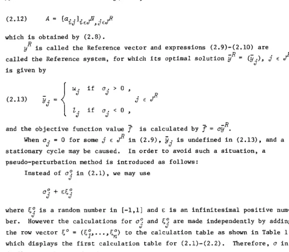
(2.12)

which is obtained by (2.8).

R

Y

is called the Reference vector and expressions (2.9)-(2.10) are

-R - .

called the Reference system, for which its optimal solution

y

=

(y.),

J J is given by (2.13) i f C. > 0 , J

EJ?

j i f c. < 0 J - - -R

and the objective function value

f

is calculated by

f

=

cy •

When c.

=

0 for some j

E J?

in (2.9),

y.

is undefined in (2.13), and a

J J

stationary cycle may be caused. In order to avoid such a situation, a pseudo-perturbation method is introduced as follows:

Instead of c~ in (2.1), we may use

J

c~

+

Et,;~

J J

where t,;~ is a random number in [-1,1] and E is an infinitesimal positive num-J

ber. However the calculations for c~ and t,;~ are made independently by adding

J J

the row vector t,;0

=

(t,;l' •••

't,;~) to the calculation table as shown in Table 1, which displays the first calculation table for (2.1)-(2.2). Therefore, c in

(2.7) should be redefined as

but since the calculations of c~ and t,;~ are made independently, we may

pre-J J

serve the definition of c as in (2.7) and define t,;

=

t,;°R-

l

=

(t,;.),

j E

J?,

J

which is calculated in the Current Calculation table as shown in Table 2.

Table 1. Starting Calculation Table

Y l ' . . . . 'Yn [0

f

J'

i'Z

CO

_u

I

-y y l - - - ---

_u

A

O

(5)

Table 2. Current Calculation Table

f

L'\fZ

y _Y

L

R Y ~OR-l cop-l R- l --- ---AOR-l

u

Since we should examine ~. only when c.

=

0 and we can practically

as-J

J

sume that ~. is not zero, then the optim.al solution for the Reference system J is now given by

u.

J i f t

_{o ,}

(c., ~.) > J J

E.r

j (2.14) t

_{o ,}

(c " ~.) -< J J Z. J i f

t

where (c.,~.) > 0 and (c.,~.)

<

0 mean lexicographic positiveness and

nega-J J J J

tiveness respectively for the bi-dimensional vectors

(c.>~.)t>

j E

.r.

-R J J

Y

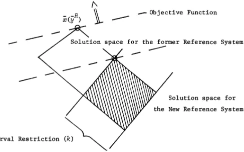
is called the Reference solution and it corresponds to a basic solu-tion satisfying the LP optimality condisolu-tion (see Fig. 1).

---

Objective function

-

Solution space for the

Fig. 1. Optimal Solution of the Reference System.

The corresponding solution

x

for (2.1)-(2.2), according to (2.5), is calculated by

(2.15) x=

_{R Y}

-l-R -N

(6)

92

(2.16) Y -N = Ay • -R

T. Sunaga. A.J. Hayakawa M. and Y. Maruki

N -R -N t

If

Y

satisfies (2.11),

(y ,y)

is a feasible basic solution satisfying the LP optimality condition and hence

X

is the optimal solution to (2.1)-(2.2). Otherwise, one variable in yN unsatisfying (2.11) must be selected to

R

enter the Reference vector and one from y to leave it.

In order to accelerate the procedure, take up the element

Yk' k

E

~

for which one of its bounds,

lk

or

u

_k

'

is the most unsatisfied one and this

Yk

enters the Reference vector. For the selection of the variable to leave the

-N

Reference vector, we have two cases when y is calculated by (2.16).

The surplus case.

Here the calculated value

Yk

exceeds its upper bound

_uk'

i.e.,

(2.17)

The value of

Yk

should be reduced in order to achieve feasibility. This is possible only when

a

_k

.

> 0 and

(c.,~.)t

> 0

(y.

=

u.),

and when

a

k

.

< 0 and

t _ J J J J J J

(c.,~.) < 0

(y.

= l.).

Therefore, pick up the lexicographic positive

bi-J bi-J J J

dimensional ratio vectors

(2.18)

(c./ak.,~./ak.)t

> 0 , j E

~

J J J J

and arranging them in an increasing lexicographic order, the following series of j is obtained:

(2.19) j(1),j(2), ••. ,j(l), •••

Next, the least index

p,

which satisfies

(2.20)

determines the variable

Yj(p)

to leave the Reference vector for this case.

The slack case.

The calculated value

Yk

falls below its lower bound

lk'

i.e., (2.21)

In a similar way as in the above case, we pick up the lexicographic negative ratio vectors

(2.22)

(c./a

k

.,

~./ak.)t

< 0, j E

~

(7)

and arranging them in an increasing lexi.cographic order with respect to their absolute values, we get the series of j given by (2.19).

Next, the least index

p,

which sati.sfies

(2.23)

determines the variable

Yj(p)

to leave the Reference vector.

In either the slack or the surplus cases, if the index

p

satisfying (2.20) or (2.23) can not be found, then (2.1)-(2.2) is infeasible. Otherwise,

Yk enters the Reference vector and Y j (p) leaves it. Next, execute an exchange operation in the calculation table by pi.voting on element a_kj(p) and a new Reference system is obtained. Following this procedure iteratively, a Refer-ence system whose optimal solution satisfies all the constraints (2.11) is obtained, or infeasibility is found. A typical two-dimensional solution space for the new Reference system is as shown in Fig. 2.

-

--- ---R

x(y )

"

t--__ Objective Function

for the former Reference System

-Solution space for New Reference System

Fig. 2. Solution space for the New Reference System.

Infeasibility test.

Before a new Reference system is obtained, an

infeasi-bility test must be executed as follows: Let us define

{":j

i f a. _ ;:.,

o ,

+

7.-J

E

,/V,

Er

(2.24) a ..

i

j 7.-J i f a __ < 0 , 7.-J

(8)

94

and

(2.25) a ..

-1--J

T. SUTIIlga. A.J. Hayakawa M. and Y. Maruki

if a .. > 0 •

1-J

i f

i

E

JV,

j E / .

When Yj' j E / takes such values as

(2.26) y. J we may write (2.27) (y.) + 1--and (2.28) (y. ) 1--if a .. > 0 • 1-J i E

JV,

if a .. < 0 • 1--J +

u.

+ E /

a-: .

EJ?

a ..

jE 1-J J jE 1--J

+

_L+

E/a:.

EJ?

a ..

jE tJ J jE 1--J L J

u.

J j E / ,

i

E

JV,

i

EJV

+

where (y.) and (y.) are the maximum and minimum of y~ respectively with

1-- 1--

<-respect to the Current Reference system. Then. i f

or

the system (2.9)-(2.11). and therefore the system (2.1)-(2.2). is infeasible and the procedure finishes (see Fig. 3).

Restriction Fig. 3. Infeasibility decision

(9)

The outline of the algorithm

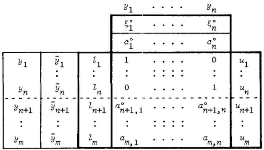
We start the procedure with the following table:

Table 1.1 Calculation Table before the Pivot Iteration.

1;;0

_{· ·}

· ·

1;;0 1 n CO

· ·

_{· ·}

CO 1 n Yl Yl l-l 1

·

0 u_l

· _·

·

· .

· ·

_·

· .

_·

Yn Yn l- 0

· _·

1 U n n

- -

-

- - - - -- -

_-

-

- - -

-

.-

- - - -

- -

-

- - - - -

-

- l-Yn+l Yn+l n+l a O n+l,l

· ·

a O n+l,n un+l

·

· .

·

· .

·

· -

l-Ym Ym _m am, 1 a _m,n u _m

Let ~ and ~ be the basic and non-basic matrices respectively, after the r-th iteration. The first basis RO is the (nXn) unit matrix in the upper

R t

part of Table 1.1. Then Y (Yp ..• ,Y_n) and Y

N

(Y_n+_{l ,··· ,Y}_m)t are the Reference and Non-Reference vectors for RO.

First, check the infeasibility by by (2.27) and (2.28) respectively. If

i E

~,

then the problem is infeasible

-R

calculating (y.)+ and

+

-z.._

(y .) - for i <:

~

-z..

(y.) < l. or (y.) >

-z.. -z.. -z.. u. -z.. for some

and the procedure finishes. Otherwise, the reference solution

Y

is read from the basic rows, as follows: If c~ > 0

J

then

y.

is read from the right-hand side on

.J

is read from the left-hand side. If c~

=

0

J

Table 1.1, and if c~ < 0 then

y.

J J

then use I;;~ instead of c~ to

J J

decide the value of

y .•

~ ~

Next, calculate

y

by mUltiplying the non-basic row vectors by

y.

If all y., i E

jl

satisfy their bounds, then

x

=

(RO)-lyR is the optimal solution

-z..

for (2.1)-(2.2). Otherwise, select the variable

Yk' k

E

~

for which one of its bounds is the most unsatisfied and it is the variable to enter the Refer-ence vector.

In order to select the variable to leave the Reference vector, compute the index p for the corresponding surplus or slack case as explained abov.~. yj(p) is then the variable to leave the Reference vector.

The Pivot element is ak,j(p) ' but since

.If

=

{I, ••• ,n} and

~

{n+l, •• ,m} in Table 1.1, we may assume that thE: pivot element is aO+

k n ,p

Now, divide the p-column by the pivot element. Add the p-column multi-plied by -a~+k, 1 to the first column, ac:d the p-column multiplied by -a~+7<, 2

(10)

96 T Sunaga, A.J. Hayakawa M. and Y. Maruki

to the second column, etc.

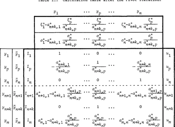
Table 2.1 Calculation Table after the Pivot Iteration.

E;,0 E;,0 E;,0

E;,0

°

e

...

e

.

..

E;,0

aO

e

1-an+k,1 aO

aO

n- n+k,n aO

n+k,p

CO CO CO cl-a~+k,l

aO

e

.. .

aO

e

...

cO-aO

n n+k,n aO

e

n+k,p

Y1

Zl

1

...

0

.

..

0

u

₁

aO

1

aO

Yp

Z

-

_ n+k,

1

..

.

...

-

n+k~n U p

aO

p

n+k,p

Yn Yn

Z

0

...

0

. ..

1 U

n

- -

-

- -

-

- -

- - - -

---_ ..

_-

-

- -

-

- - - -

-

--aO

aO

Yn+1 Yn+1 Z

n+1 n+1,1 n+k,l aO

aO

-ao

n+1~e

_n+k,p

...

aO

n+1.ze

_n+k,p

...

aO

n+1,n n+k,n aO

-ao

n+1,p

_n+k,p

un+1

Yn+k Yn+k Z n+k

0

...

1

...

0

un+k

aO

Ym Ym Z

m

aO

m,l n+k,l aO

-ao

m.z"fi.

..

.

aO

m.z"fi.

...

aO

m,n n+k,n aO

-ao

m.z"fi.

u

m

n+k,p

The table obtained after applying the above pivot operation is as shown

-R

in Table 2.1, where the new solution

Y

is read in the same fashion as before. Observe that in the ea1cu1ation table the elements of Y are not rear-ranged and the pivot operation affects only the coefficients' matrix and the row vectors E;,0 and

co.

TIle bounds are not changed because the table has the form

where the values of

Yi'

i

=

1, ••.

,m are moving toward feasibility, and any change in the bounds means a redefinition of the original problem.

2.1 Interval width reduction procedure

This proce.dure was introduced by Zionts [6] in order to accelerate the solution of integer LP problems. Availing the calculation of (2.27) and

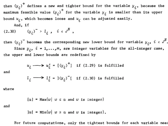
(2.28) in the infeasibility test explained above, we have that, if (2.29)

(11)

+

then (y.) defines a new and tighter bound for the variable Y

i'

because the

~

+

maximum feasible value (Yi) for the variable Yi is smaller than its upper bound

u

_i

'

which becomes loose and

u

_i

can be adjusted easily.

And, if

(2.30) (y.)

>L,

iEJV,

~ ~

then (Yi) becomes the corresponding new lower bound for variable Yi' i E

JV.

Since

y.,

i

=

l, ••• ,m, are integer variables for the all-integer case,

~

the upper and lower bounds are redefined by

u!

+

i f (2.29) is fulfilled U.~ [(Yi) ] ~ ~ and l. ~ l! ](Y i )

-

[ if (2.30) is fulfilled ~ ~ where

[cd Max{w / w ::; a and w is integer} and

]a[ =

Min{w/ w

~ a and

w

is integer},

For future computations. only the l:ightest bounds for each variable need be remembered. The interval width reduetion means a substantial reduction in

the set of feasible solutions for the rE~laxed problem as shown in Fig. 4.

Reference System

y. =

z..

~ ~

Fig. 4 Interval Width Reduction

Some simple examples can be solved by simply utilizing this procedure as shown in the following example:

(12)

98 T. Sunaga. A.J. Hayakawa M. and Y. Maruki

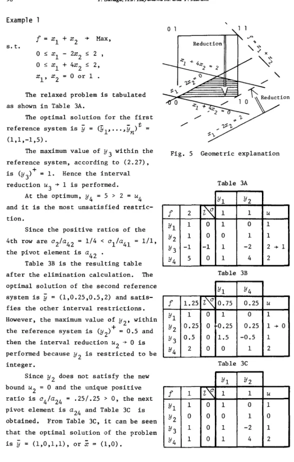
Example 1

f= s. t. xl

+

x₂ + Max, 0 :,; _x -1 2x2 :,; 2

,

0 :,; _xl

₊

_4x 2 :,; 2, xl' x 2

o

or 1

.

The relaxed problem is tabulated as shown in Table 3A.

The optimal solution for the first

-

t

reference system is y = (11

1, .. . ,yn)

(1,1,-1,5) .

The maximum value of Y

3 within the

reference system, according to (2.27),

+

is (Y

3)

=

1. Hence the interval reduction u

3 + 1 is performed.

At the optimum, Y4

=

5 > 2

=

u₄

and it is the most unsatisfied restric-tion.

Since the positive ratios of the 4th row are c₂/a₄₂

=

1/4 < c₁/a₄₁

=

1/1, the pivot element is a

42 .

Table 3B is the resulting table after the elimination calculation. The optimal solution of the second reference system is

y

=

(1,0.25,0.5,2) and satis-fies the other interval restrictions. However, the maximum value of Y2' within

the reference system is (Y

2)+

=

0.5 and then the interval reduction u

2 + 0 is

performed because Y

2 is restricted to be

integer.

Since Y2 does not satisfy the new bound u

2

=

0 and the unique positive

ratio is

c

₄

/a

₂₄

=

.25/.25 > 0, the next pivot element is a₂₄ and Table 3C is obtained. From Table 3C, it can be seen that the optimal solution of the problem is

y

=

(1,0,1,1), or

x

=

(1,0).

,

o

1

Reduction

Fig. 5 Geometric explanation

Table 3A Y1 Y2

f

2

z"\

1 1 u Y1 1 0 1 0 1 Y2 1 0 0 1 1 Y₃ -1 -1 1 -2 2 + 1 Y4 5 0 1 4 2 Table 3B Y1 Y4

f

1.25

i'\

0.75 0.25 u Y1 1 0 1 0 1 Y2 0.25 0 0.25 0.25 1 + 0 Y₃ 0.5 0 1.5 -0.5 1 Y4 2 0 0 1 2 Table 3C Y1 Y2

f

1

z'\

1 1 u Y1 1 0 1 0 1 Y2 0 0 0 1 0 Y 3 1 0 1 -2 1 Y4 1 0 1 4 2

(13)

The geometric explanation of the calculation procedure is shown in Fig. 5. The perturbation method is not used in this example; it will be explained in a later example.

The method explained in this section will be called the Modified Interval Linear Programming (MILP) method for future references.

3. Gomory's Fractional Cut for IILP

This section explains the app1icati.on of Gomory's Fractional Cut to Integer Interval Linear Programming.

We suppose that (2.1)-(2.2), the relaxed problem of (1.1)-(1.4), is solved by the MILP method explained in Section ,2 and that its optimal solution

- _ (_R _N)

t

" _

,

_ ,

x

in terms of y

= Y

,y and the coeff:icients o. s and

a . .

s corresponding

J 1.-J

to the last reference system (2.9)-2.10) are available.

Since

yR

is always integer, then the integrality of

yN

is the necessary

- - - )t

and sufficient condition in order for x

= (Y1""'Yn

to become the optimal solution to (1.1)-(1.4).

If

yN

is not integer, select one element Yk' k E

jV

whose value Yk is not integer; the equation associated to Yk "rill be referred to as the Source Row.

Consider the fractional parts fk and f

kj such that

(3.1) and

(3.2)

Now from Yk

=

E J?

a

k ·

y.,

Yk

=

E J?

a

k-,

y.

and the expressions (3.1)-(3.2),

jEJ" J J jEtT" 0) J

we have that (3.3)

and

Let us define

J+

and

J-

as follows:

J+

= {j

I

j E

.I

and (0., f, .)

t

>" O}

J J

[

=

{j

I

j E

.I

and (0., f, .) t <: O},

J J

then from (3.3) we obtain the next expression (3.4)

(14)

100 T. Sunaga, A.J. Hayakawa M. and Y. Maruki

In order for

Yk

and

Yj'

j €

~

to be integers, a necessary condition is

that the right-hand side of (3.4) must also be integer.

From the determination of Yj' j E

~

by (2.14), it is easy to verify that if j €

J+

then

(y.-y.)

$ 0 and if j €

J-

then

(y.-y.)

~

O. Hence we may write

J J J J

(3.5)

and the necessary condition for integrality becomes (3.6)

So, we get the Interval Fractional cut (3.7)

which is added to the current system (2.9)-(2.11). The expression (3.7) shall be referred to as an F-cut.

The 1eft-han side of (3.7) must be an integer because all the interval bounds,

l.'s

and

u.'s,

must be integers in the initial calculation table.

'l-

'l-Hence we must show that

is an integer.

From expression (3.1) and (3.2), we have

and thus

Since the left-hand side is an integer, (3.8) must be an integer.

After adding an F-cut to the current system, it is reoptimized by the MILP method and a new solution

x

is obtained.

By applying iteratively the procedure explained above, after a finite number of iterations the optimal solution to (1.1)-(1.4) should be reached. However, this method has the same numerical troubles as various cutting plane methods in Integer Linear Programming. Hence it is combined into a Search procedure, whose purpose is to improve the computational efficiency.

(15)

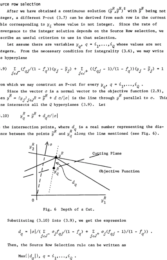
Source row selection

_R_Nt. _N

After we have obtained a continuous solution (y , y ) w1th y being not integer, a different F-cut (3.7) can be derived from each row in the current table corresponding to y

i

whose value is not integer. Since the rate of convergence to the integer solution depends on the Source Row selection, l.e describe an useful criterion to use in that selection.

Let assume there are variables

Yq' q

= il, ••. ,i

Q

whose values are not integers. From the necessary condition for integrality (3.6), we may write the hyperp1ane

(3.9) ~ (f ./(1 - f »(y. - fJ·)

+

~+ « f . - 1)/(1 - f »(y. - fJ·)

jEJ- qJ q J J jE<l qJ q J J 1

from which we may construct an F-cut for every Y_q' q =

i

_{lP ••}

,i

Q

Since the vector a is a normal vector to the objective function (2.9), then yR

=

(y.).

~

=

fJR

+

d a/lal is the line through yR parallel to a. 'This

J

JE,;-line intersects all the Q hyperp1anes (:\.9). Let (3.10)

be the intersection points, where d is a real number representing the dis-R R q

tance between the points

y

and y _qalong the line mentioned (see Fig. 6).

~ting Plane

----

Objective Function

o

Fig. 6 Depth of a Cut.

Substituting (3.10) into (3.9), we get the expression d

q lal/( jEJ ~ _ a·f J qJ ./(1 - f ) q

+

jEJ ~

+

a ·(f . -J qJ 1)/(1 - f q

»

(16)

The effort required by this criterion to select the new source row can be justified by the improvement in the rate of convergence (see Section 5).

4. The Search Procedure

In this section we describe the Search procedure, which uses the IILP method described in sections 2 and 3. As mentioned in Section 1, the purpose of the Search procedure is to solve problem (1.1)-(1.4). The procedure con-sist of two steps.

First, consider that the relaxed problem (1.1)-(1.3) is solved by the MILP method and its continuous solution

x

is obtained, now let us define

which are the continuous and the integer upper bounds for

f

in (1.1) respec-tively.

The continuous lower bound ~ for

f

in (1.1) can be calculated by using

instead of (1.1). Now let x . be the optimal solution to the minimization

I111.-n

problem, and ~ is defined as

~

Step I

The purpose of this step is to find an upper bound

fO.

Since (1.1)-(1.3) is a bounded problem, the MILP method finds its finite optimal solution or its infeasibility. If X is obtained, the upper bound

fO

is at hand and we proceed to Step 11. Otherwise infeasibility is detected, the problem (1.1)-(1.4) is also infeasible and the procedure finishes, because continuous infeasibility implies integer infeasibility.

Step 11

In this step we search for the integer optimal solution to problem (1.1)-(1.4). Let S be the set of feasible solutions for problem (1.1)-(1.4), Le.,

S

=

{xl

l

5

A'

x 5 u and x is integer}. Now consider the subsets 8

t

of S

(17)

St

=

{xl

l

~

A' x

~

u, cox

=

f

_t

and

x

is integer} where

f

t

is an integer such that

fl

=

fO

and

f

t

=

ft_I-I,

for t

=

2,3, ... ,T,

and

fT

is an integer lower bound for

f

in (1.1), defined as

fT

=

If-[.

Since the elements in CO are all-integer, then

T

S

= u

St

t=l

and the optimal solution to (1.1)-(1.4), if it exists, must be in some subset

St'

t

=

1, .•• ,T.

We shall examine the subsets

St

in sequence. The purpose of this examina-tion is to get a tighter upper bound

fO,

which is now

fO

=

f

_l

•

If we may show that the subset

SI

does not contain any integer feasible solution, then we set

fO

= f

2 ,

if the subset

S2

does not dontain any integer feasible solution,

then

fO

=

f3'

and so on. Therefore, when an integer feasible solution is found, this solution is the optimal one for problem (1.1)-(1.4).

In order to examine the subsets

St'

'we may use the IILP method. For this purpose, consider the sequence of artificial optimization subproblems PI""

,PT'

where the subproblem

Pt

is (4.1)

F

=

g(x , ••• ,x

n

)

~ Max, s.t. (4.2) l. ~

x.

~

_u.

,

_i

1, ... ,

n,

'!.- '!.-

'!.-n

(4.3) _lk~ L:

a

_kj

x.

~

u

k ' k

+

n+l, ... ,m,

j=l J

n

(4.4)

_f

t

~ L:

c.

°

x.

~

f

t

,

j=1

J J (4.5)

x.

is an integer j 1, ...

,n

J

where,g(xl, ••• ,x

_n

)

is any linear function with all-integer coefficients. For instance:

g(x)

=

xi

or

g(x)

=

j~l

ahjx

_j., for some h

=

n+l, .•• ,m.

Subproblems

P1"",P

_T

are solved in sequence by the IILP method, which has only two possible results, integer fl~asibility or integer infeasibility. Consider the subproblem

Pt;

if an integer feasible solution is found, this solution is the optimal one for problem (1.1)-(1.4) and the procedure fin-ishes. Otherwise integer infeasibility is found, it means that all the con-tinuous feasible solutions in the hyperplane

cox

= f

_t

were cut off by the cutting planes. Therefore, we proceed to the ne}ft subproblem P

(18)

Since subprob1ems

P

1 •...• P

T

are artificial optimization problems to find

their integer feasible solutions, we may introduce the following procedure in order to accelerate the search of integer feasibility.

Since the cutting planes lose effectiveness gradually, for some problems even though

X

is near to the optimal solution

x,*

it still takes a long time until

x*

is recognized. Hence, we examine the feasibility of the rounded solution

z,

which is defined as

where f! is

"Z-+

1 i f i f

f

_"Z-! >- 0 5 _• f! < 0.5

"Z-x.

=

[x.]

+

f ! ; 0 $ f! < 1. "Z- " Z - " Z -

"Z-If Z satisfies (4.3) and (4.4), then

z

is an integer feasible solution and the procedure finishes. Otherwise, we proceed to introduce a new cutting plane to search for a new continuous solution

X. Algorithm

STEP I. Solve the relaxed problem (1.1)-(1.3) by the MILP method in Section 2, here cutting planes are not used. One of the following three cases is obtained:

i) INTEGRALITY. The optimal solution

x

for the relaxed problem is integer. Hence

x

is the optimal solution to (1.1)-(1.4) and the procedure finishes. ii) INFEASIBILITY The relaxed problem is infeasible. Since continuous in-feasibility means integer inin-feasibility, the procedure finishes and (1.1)-(1.4) is found infeasible.

iii) CONTINUOUS FEASIBILITY.

x

is not integer. Then

is an upper bound for

f

in (1.1). Solve the minimization problem mentioned above, whose solution provides

f-.

Set t

=

1 and go to step 11.

STEP 11. Solve subprob1em Pt' i.e., problem (4.1)-(4.5) by the IILP method. As described previously, evaluate the rounded solution

z

from every continuous solution

x

obtained. Here one of the following two cases becomes:

i) INTEGER FEASIBILITY. An integer solution

x*

for (4.1)-(4.5) is obtained. Since

f* = cox*

=

f

_t is an upper bound for

f

in (1.1),

x*

is the optimal solution to (1.1)-(1.4).

(19)

ii) INTEGER INFEASIBILITY. The subproblem Pt is found to be integer infeasi-ble. I f

f

t is equal to the lower bound .fT' the procedure finishes and

(1.1)-(1.4) is infeasible. Otherwise, ft+l

=

.f

t - 1 becomes a new upper bound for

f,

because for higher values of

f

there is no integer feasible solution. Set

t

=

t

+

1 and go to the starting point of step 11.

Example 2

Consider the problem

f

=

5x l

+

l3x2

+

5x3

+

4x4

+

3x5

+

7x6 ~ Max, s.t. 3x l

+

4x2 + l6x3 + 7x4 + 7x5 + 6x6 $ 25 , Xi

=

0 or 1, i 1, ... ,6

STEP I, The continuous relaxed problem is formulated as an ILP problem and solved by the MILP method. The continuous solution

x

is obtained and the objective function is f+

=

31.143.

STEP 11. Consider the subproblem Pt

s.t.

o

$ 0 $ 3x l

+

4x2

+

f

_t

$ 5x l

+

l3x2

+

x. is an integer, 'Z-l6x 3 X.

'Z-+

7x 4 SX 3

+

4x4

+

i

= 1, •.• ,6. $ 1 i 1, ••• ,6, 7x 5

+

6x6 $ 25 3x S

+

7x6 $

f

t

,

Searching for integer feasibility in fl

=

r

=

31 and f2

=

30, by the IILP method, we find that both subproblems PI and P

2 are integer infeasible.

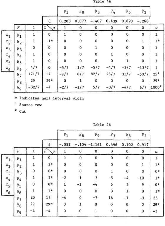
Hence, following the Search procedure, subproblem P

3 with f3

=

29 is examined.

Table 4A shows the optimal continuous solution for subproblem P

3, where

in the last row a cut is added because the rounded solution

z

=

(1,1,0,1,1,1) is infeasible. Finally, Table 4B shows the integer optimal solution.

(20)

106

xl

x

2 x3

x

₄

x5

x6

xl

x

₂

x3

x

₄

x5

x6

'

-T. Sunoga. A.J. Hayakawa M. and Y. MllTUki

Table 4A

Y1

YS

Y3

Y4

~ 0.20S 0.077 -.407 0.439 F 1

l y

1 0 0 0

Y1

1 0 1 0 0 0

Y2

1 1* 0 0 0 0

Y3

0 0 0 0 1 0

Y4

1 0 0 0 0 1

Y5

1 0 0 0 0 0

Y6

4/7 0 -5/7 1/7 -5/7 -4/7

Y7

171/7 17 -9/7 6/7 S2/7 25/7

YS

29 29* 0 1 0 0

Y9

-32/7 -4 -2/7 -1/7 5/7 -3/7

*

Indicates null interval width

Source row 2 Cut F 1

Y1

1

Y2

1

Y3

0

Y4

1

Y5

0

Y6

1

Y7

20

YS

29

Y9

-4 ~

l~

0 1* 0* 1* 0* 1* 17 29* -4 Table 4B

Y1

YS

Y9

Y3

-.051 -.104 -1.161 0.496 1 0 0 0 1 0 0 0 0 0 0 0 0 0 0 1 -2 1 3

-5

1 -1 -4

5

0 0 0 0 -4 0 -7 16 0 1 0 0 0 0 1 0

Y5

Y2

0.620 -.26S 0 0 u 0 0 1 0 1 1* 0 0 1 0 0 1 1 0 1 -3/7 -13/7 1 31/7 -50/7 251 0 0 29* -4/7 6/7 10002

Y6

Y2

0.102 0.917 0 0 u 0 0 1 0 1 1* 0 0 0* -4 -10 1* 3 9 0* 1 0 1* -1 -3 23 0 0 29* 0 0 -3

(21)

5. Computational Results

To evaluate the performance of the proposed method, we use twenty-nine test problems from four groups,

A) Nine Allocations Problems

B) Ten Fixed-Charge Problems of Haldi

C) Four Combinatorial Problems in Graph Theory D) Six "IBM" Test Problems of Haldi,

which are explicitly reproduced in C.A. Trauth, JR. and R.E. Woolsey [5]. We shall evaluate our results based on the results published in the above reference, where the used codes and other features are detailed. Here we re-produce only some features which help us: to evaluate the performance of the Search procedure.

In reference [5], the following five codes are tested: IPM 3 and LIP 1, which are based on the Gomory's fractional cut, and ILP 2-1, ILP 2-2 and IPSC, which .are based on the Gomory' s all-inte'ger cut.

Tables 5, 6, 7 and 8 show the results published in the above reference and the results obtained by the Search procedure, for each group of problems tested, where iteration means a pivot iteration.

For the Search procedure, the random number series are arbitrarily chosen and

F

=

xl in Step 11 is used for all the tested problems. We use two experi-mental codes for the Search procedure; the first one is written in BASIC and a personal computer NEC PC-8801 (P) is used and the reported CPU time for this code includes the display time. The second code is written in FORTRAN 77 and it is run on a large scale computer FACOM M382 (L). For this case, the reported CPU time includes compilation.

Considering differences among machi.nes, a comparison on basis of calcu-lation time lacks meaning. However the CPU time is reproduced to give an idea of the invested effort.

The Search procedure managed to solve all the above test problems, espe-cially the 7-point combinatorial problem, which became infeasible.

The Search procedure shows computational stability for small size pro-blems as seen in the test propro-blems solved. However, in future, applications

(22)

108 T. SUTIilga, A.J. Hayakawa M. and Y. Maruki

Table 5. Allocation Problems

Code

IPM 3 Problem Size Iter.

1 1X10 14 2 1X10 31 3 1X10 30 4 1X10 18 5 1X10 11 6 lXI0 18 7 1XI0 61 8 lX10 21 9 1X10 12 Time in seconds Size means (m-n)Xn LIP 1 Iter. 19 55 41 19 12 40 81 51 12 !LP ILP 2-1 2-2 IPSC Iter. Iter. Iter.

54 51 46 163 77 64 168 59 71 192 48 62 139 32 50 157 54 81 504 119 131 307 57 102 201 34 44 Search Procedure Iter. Time Machine

5 71 P 32 380 P 22 197 P 12 118 P 3 52 P 25 256 P 39 404 P 29 280 P 4 120 P

Table 6. Fixed-Charge Problems

ILP !LP Code

IPM 3 LIP 1 2-1 2-2 IPSC Search Procedure Problem Size Iter. Iter. Iter. Iter. Iter. Iter. Time Machine

1 4X5 54 24 135 36 32 22 171 P 2 4X5 81 15 94 47 45 19 120 P 3 4X5 37 26 154 104 56 22 132 P 4 4X5 91 18 93 18 22 19 120 P 5 5X5 +7000 158 +7000 +7000 6104 124 800 P 6 5X5 +7000 123 +7000 311 3320 101 540 P 7 3X5 +7000 159 +7000 +7000 +7000 124 800 P 8 3X5 +7000 126 +7000 306 +7000 101 540 P 9 6X6 118 42 +7000 298 339 58 485 P 10 10X12 1369 102 +7000 +7000 +7000 94 2170 P Time in seconds

(23)

Table 7. Combinatorial Problems

Code ILP ILP

IPH 3 LIP 1 2-1 2-1 IPSC Search Procedure Problem Size Iter. Iter. Iter. Iter. Iter. Iter. Time Machine

4-Point 4X6 4 11 4 4 5 6 56 P

5-Point 4XlO 140 83 132 74 86 52 1080 P

6-Point 65X15 42 27 114 29 70 51 2.5 L

7-Point l40X21 +7000 +7000 +7000 +7000 +7000 2830 24.0 L Time in seconds

Table 8. "lBW' Test Problems

Code ILP ILP

IPM 3 LIP 1 2-1 2-2 IPSC Search Procedure Problem Size Iter. Iter. Iter. Iter. Iter. Iter. Time }1achine

1 7X7 8 11 9 11 9 13 129 P 2 7X7 17 32 13 15 16 26 240 P 3 3X7 22 53 23 14 14 65 338 P 4 l5X15 24 73 41 18 17 40 737 P 5 l5X15 1144 351 +7000 842 1020 224 2.7 L 9 35X15 6758 953 +7000 1105 752 562 3.7 L Time in seconds

Acknowledgment

The authors are grateful to the referees for their valuable comments on this paper. The second author is partially supported by the National Council of Sciences and Technology of the Mexican Government (CONACYT) and by the Durango's Institute of Technology (l1exic:o) during his studies in Japan as a schoolarship student of the Japanese Ministry of Education.

ReferE!nCeS

[1] Ben-Israel, A. and Charnes, A.: An Explicit Solution of a Special Class of Linear Programming Problems. Operations Research, Vol.16, No.6 (1968)

, 1166-1175.

(24)

Inter-110 T. Sunaga. A.J. Hayakawa M. and Y. Maruki

val Linear Programming Problems.

Operations Research,

Vol.25, No.4 (1977) , 688-695.

[3] Garfinkel, R. and Nemhauser, G.L.: A Survey of Integer Programming Empha-sizing Computation and Relation among Models.

Mathematical Programming

(eds. T.C. Hu and S.M. Robinson). Academic Press, 1973, 77-155.

[4] Taha, H.A.:

Integer Programming, Theory, Applications and Computations.

Academic Press, 1975.