Primal duai method of parametric programming and iri′s theory on network flow problems

Journal of the O. R. Society of Japart Vol. 7, No. 3, February 1965.

PRIMAL DUAL METHOD OF PARAMETRIC PROGRAMMING AND IRI's THEORY ON NETWORK FLOW PROBLEMS

By REIJIRO KURATA RAND Inssitute oJ jUSE, Tokyo

INTRODUCTION

Primal dual algorithm of linear programming problems was first applied to the network flow problem by Ford and Fulkerson [2] [3]. In 1959, Kelley [1] pointed out that this is nothing but a method for solving parametric programming problem. In § 1, we shall describe the primal dual method of parametric programming in a general fashion. The con-tent is essentially the same as that of [1], except for that the simplex method and the concept of basis are avoided, as they are not neccessary for our discussions and we treat the "general form" of the linear pro-gramming. This method was applied by Kelley [4] and Fulkerson [6] independently of each other, to a problem in planning and scheduling, which is now called CPM (Critical Path Method).

On the other hand, in 1960, Iri studied the network flow problem from an entirely different viewpoint. He developed a general algebraic and topological theory of electric circuit and noticed the analogy of the transportation problem with the circuit.

A few important points should be noted about Iri's theory. The first of them is his methodology. In his theory, the input voltage and total input current are increased alternatively starting from

°

so that the solutions of problems are found out. A technique called "e-matrix method" used at the voltage increasing steps forms the most important part in [5]. Iri's alternative increasing steps are regarded as an illustra-tion of a method which is applicable to the general problem of parametric

104

Primal Dual ]}[ethod of Parametric Programming 105 programming.

In § 2 we introduce this method, under the name "double para-metrization method ", and show that it is as equally efficient as the method in § I in the sense that the number of iterations to reach at a parameter value A is the same for both the methods. In general, in formulating a parametric programming problem, various ways are possible according as which variable is taken as a parameter. For instance, if the input voltage is taken as the parameter of the network flow problem we get Ford and Fulkerson's method. A different approach, of course, is obtained if the total flow is taken as a parameter. In the former, the maximal flow is found by a labeling method which is well-known as one for solving the restricted primal problem, while in the latter, the maximal input voltage is found by the El-matrix method.

J

liSt as the labeling method in Ful-kerton's theory gives the optimal solution of not only the restricted primal problem but also its dual problem, El-matrix method gives the optimal solutions of both the restricted primal and the dual problems simultaneously (this fact is not remarked in [5]). These two methods are discussed in § 3.

In § 4, we apply Kelley-Fulkerson's and Iri's methods to the problem of CPM in parallel to § 3. Iri's method in CPM has not yet been pub-lished. Iri himself, however, was aware of the possibility of the application as early as in 1961 and wrote an ALGOL program at the RAND Institute of JUSE, Tokyo. It is shown in § 5 that if we apply the primal dual method directly to the problem with many parameters, a certain very strong condition on the solutions of restricted primal problems is required. However, if we regard the network flow problem with many sources as a multi-parametric programming problem with many input flows as parameters, the condition above stated is fulfilled. Thus it is the third feature of Iri's method that his El-matrix method can be applied to the network flow problem as a multi-parameter programming, as discussed in §6.

Transportation problem of Hitchcock-type turns quite naturally to be a multi-parameteric programming, for which a numerical example

106 Reijiro Kumta

solved by the method in § 6 is attached in § 7.

§ 1. PRIMAL DUAL METHOD OF PARAMETRIC PROGRAMMING IN GENERAL FORM

Let PI..l and DI..l denote respectively the following parametric pro-gramming problem and its dual problem.

PI..l Xj~O if jES (PI)

'E.aijxj~bi ,

if

iET'}

j

(or 'E.aijXj-ui=bi, Ui~O, if iET,) (P2)

j

'E.aijxj=b i , if i$T,

j

mlmmlze f(x)

=

'E.

(Cj+,{dj)Xj, (P3)

j

DI..l

'E.

aijYi;;?,Cj+,{dj, if

jES, }

i

(or 'E.aijYi+Wj=Cj+,{dj, Wj~O, if jES,) (Dl)

;:'aijYi =Cj+,{dj, if j$S,

Yi~O, if iET, (D2)

maximize g(y)

=

'E.

yibi , (D3)

where i ranges over the set of integers {I, 2, ... , m} and j over {l, 2, ... , n}, and T(resp. S) is a given subset of {I,2,···,m} (resp. {I,2,···,n}).

1.1. Our aim is to trace the optimal solution of PI..l or DI..l, when ..l increases from ..lo, being given the optimal solution of Pl..lo or DI..lo.

Let (x], u,) and (Yi, Wj) be the optimal solutions of PI..l and DI..l respectively and let us define the restricted primal RPI..l and its dual restricted problem RDI..l, based on (Yi, Wj), as follows.

RPI..l

Primal Dual Method of Parametric Programming 107

'E.aijxj~bi , if iET,

1

j

(or 'E.aijXj-Ui=bi , Ui~O, if iET,) (RP2) j 'E.aijxj=bi, if i$T j

'E.

XjWj=O,

1

jES (RP3)

'E.

UiYi=O, iET minimize j;(X)

=

L;.dJxj. (RP4) J RDIA

'E.aijai~dj , if Wj=:O, and jES,

1

(RD1) l;.aijai=dj , if j$S

ai~O, if Yi=O and iET, (RD2)

maximize h(a)

=

'E.(/ibi . (RD3)

i

Proposition 1. 1.

A feasible solution (.:>:j, Ui) of P I ~ is optimal, if and only if it IS a

feasible solution of RPIA.

Proof.

If (x), Ui) resp. (Yi, Wj) is a solution of PIA resp. DIA, then we have easily 'E.(Cj+Adj)Xj= 'E.biYi+

'E.

WjXj+ l~ UiYi, and

'E.

WjXj~O,

'E.

UiYi~O.

j i jES iE,T jES iET

By the Duality Theorem, (Xi> Ili) is optimal, if and only if

'E.

WjXj=O

jES

and

'E.

UiYi=O, that is, (x), Ui) is a feasible solution of RPIA.

iET

Proposition 1. 2.

If (y;') is a feasible solution of DIA+O for some 0>0, and if (ai) satisfies (Y/)=(Yi)+O(ai), then (ai) is a feasible solution of RDI~.

Proof.

By our assumption, (Yi+O(/i), is a feasible solution of DIA+O. SO that,

108 Reijiro Kurata

I:

aij(Yi

+

OlJi)-;:;;;'Cj+ (..l

+

O)dj

i for for for jES, iET (1. 1) (1. 2)

Cl.

3) From (1. 1) and (1. 2) (I:aijlJi-dj)O-;:;;;'Wj i (I:aijlJi-dj)O=O i for for Hence ai is a feasible solution of RDI.l.

Proposition 1. 3.

jES, (1. 4)

jetS. (1. 5)

Let (ai) be a feasible solution of RDI.l and put (f3j) = (dj - 2;:aijai),

then (y+Oai) is a feasible solution of DI.l+O (0)0), if and only if 0<0-;:;;;'00

where 00 is defined as follows.

{

minC-WJ/{3J; (3j<O, jES) if there existsj such that _8J<0, 01

=

<Xl otherwise,

{

min(-y;/ai; ai<O, iET)

O2=

<Xl

Oo=min (01)

°

2).

Proof.

if there exists i such that ai<O, otherwise,

Note that 01>0 and O2>0, because {3j<O implies Wj>O for jES,

and lJi<O implies Yi>O for iET, by RDI and RD2. Now from the proof of Proposition 1.2, (Yi+Oai) is a feasible solution ofDI.l+O, if and only if (1. 3) and (1. 4) hold, that is if and only if 0-;:;;;'01 and 0-;:;;;,02.

Proposition 1. 4.

Suppose that 0<0-;:;;;'00 , where 00 is defined as in Proposition 1. 3, and

that (x}) is a solution of RPI..l. Then (Xj) resp. (Yi+Oai) is an optimal feasible solution of PI..l+O resp. DI..l+O, if and only if (Xj) resp. (ai) is an optimal solution of RPI..l resp. RDI,l.

Proof.

Primal Dual Method of Parametric Programming 109 Theorem imply the proposition.

f(x) = L:(Cj+(A+O)dj)xj= L:bi(Yi+Oai)=g(y+Oa)

j i

Proposition 1. 5.

If the optimal solutions of PIA and DIA exist for some A, the neccessary and sufficient condition for the existence of the optimal solutions of PIA' and DIA', ..i'>A, is the existence of the optimal solutions of RPIA and RDIA.

Proposition 1. 6.

An optimal solution of RPIA is a feassible solution of RPIA+O where

0<°:;;;'°0'

Proof.

Let (xj, Ui) resp. (a i) be the optimal solution of RPIA resp. RDIA, then (yt', w/) defined by

yt'=yt+Oai,

w/=Wj+O~j for jES,

is the optimal solution of DIA+O. For, from Dl with ..1+0 for jES.

(1. 6)

To prove that (xj, Ui) is a feasible solution of RPIA+O, it suffices to show that (1. 7)

L:

UiYt'=O. iET (1. 8) Now by (1. 6)

110 Reijiro Kurata and

While for an optimal solution (Xi> Ui) resp. (ai) of RPIA resp. RDIA, we have

I:

Xj{3j=O and

I:

uiai=O because from RPI-3 and RD-2,

jES iET

and

therefore,

I:

aiui=O and

I:

{3jXj=O by the Duality Theorem.

iET jES

Thus we can formultate the following procedure to solve PIA or

DIA-l. Start with an optimal feasible solution (Xi> Ui) resp. (Yi, Wj) of PIA resy. DIA for some A.

2. Construct RPIA and RDIA making use of (Yi, Wj).

2a) If taere is no optimal solution of RPIA and RDIA (e.g. RPIA has no bounded solution) then, there exists no optimal solution of PIA' and DIA' for ;('>A. In this case, give up the procedure.

2b) When we can get optimal solutions (x;, Ui) resp. (a,:) of RPIA resp. RDIA, put {3j=dj- I:aijai,

i

{

min(-Wj/{3j; (3j<O, jES), 01 =

00,

{

min(-Yi/ai;

a,<O,

iET), O2

=

00,

and

3.

if there exists j E S such that {3 j<O, otherwise,

if there exists iET such that ai<O, otherwise

Primal Dual Method of Parametric Programming III solution of PjA+O resp. DI;(+O for any 0>0. Thus, the procedure is terminated.

3b) If 00

<=

then (Xi> Ui) resp. (Yi+OO"i, Wj+Oo[3j) is an optimal solution of PI;(+Oo resp. DIA+O. In this case return to step 2 (and here, Proposition 1. 6 is very useful), and continue the process.

1.2. Next we shall get the optimal tolution of PI2' or DjA', ;('<2, starting with the optimal solution of PIA and DI;(.

This time we consider the following RP'I;( and RDI;(. RP'I;( (or RD'I;( Xj~O, if jES, L:aijxj~bi, if iET,

}

j

L:aijX-ui=bi, Ui~{), if iET,)

j

L:

aijXj = bi, if i$T,

j

I

maximize

if Wj=O and jES,

I

if jEES,

if y,=O and iET, minimize h( a) ==

L:

a ibi •

j

In this case Oh O2 and 00 are defined as follows.

(RPl) (RP2) (RP3) (RP'4) (RD'l) (RD'2) (RD'3)

if there exists jES such that [3j>O, otherwise,

112 Reijiro Kumta

if there exists iET such that l1i>O, otherwise,

Moreover, for 0, O<O:;aOo, (x}, Ui) resp. (Yi-Ol1i, Wj-O~j) is an optimal solution of PIA-O resp. DIA-O.

§ 2. A METHOD OF DOUBLE PARAMETRIZATION

Again, we consider PIA and DIA, and now we introduce a new varia ble p in PIA.

Xj;;;;:;O, 'Laijxj~hi,

j

(or 'LaijXj-ui=hi, Ui~O,

j

'L

aijXj= hi,

j

minimize f(x, p)= 'LCjXj-Ap.

j

(or 'LaijYi+Wj=cj+Mj, Wj~O,

i.

RPIA

'LaiiYi=Cj+Mj,

i

maximize g(y)= 'LhiYi.

j if jES if iET if iET), if i$T, if jES, if jES,) if j$S, if iET, if jES,

}

]

(PI) (P2) (P3) (P4) (Dl) (DT) (RPI)

Primal Dual Method 01 Parametric Programming

.Ea,jxj';;;j;,bi , if

iET,

}

j

(or

.E

aiJX) - Ut

=

bi , Ut';;;j;,O, if

iET,)

(RP2)

j .EaijxJ=bl • if

i$.T,

j - .EdjxJ=p, j (RP3)

.E

xJWj=O,

f

jeS _(RP4)

.E

UtY,=O, leT minimize -po (RP5) RD/A

.Eaijai~dj, if Wj=O and

JES,

}

i _(RD)

.Eaijai=d, if

j$.S,

i

a,';;;j;,O, if Yi=O and

iET,

(RD2)

maximize h(a)= .EbWt.

i (RD3)

Now in PIA, we regard p as a parameter, and consider the following problem D*lp Xi :?;O, if

JES,

(D*l)

.E

aijXj:?; bi , if

iET,

}

j

(or .Eaijxj-ui=b" Ut :?;O, if

iET,)

(D*2)

i

.E

atjxj= hi, if i$.T,

j

-~djxj=f!., (D*3)

J

minimize f*(x}= .ECjXj. (D*4)

114 Reijiro Kurata

The primal problem P*I,u which is the dual of D*I,u is defined as follows. Here, A is regarded as a variable corresponding to (D*3).

P*I,u

'[.aijYi~Cj+Adj, if jES,

}

,

(or .'[.aiiYi+Wj=Cj+Adj, Wj~O, if jES,) (P*l) "

'[.ai,iYi=Cj+).dj, if j$S,

i

Yi~O, if iET, (P*2)

maXImIze g*(y, A)= '[. yibi+ ,uA.

_,

(P*3)

RP*I!I

'[.aijYi+Wj=Cj+Adj, Wj~O, if iES,

t

,

_(RP*l)

'[. taijYi= Cj+Adj,

_,

IS jES,

Yi~O, if iET, (RP*2) '[. WjXj=O,

t

jES _(RP*3) '[. YiUi=O, iET maximize A. (RP*4) RDI*,u

;j~O, if Xj=O and jES, (RD*l)

'[.aij~j~O, if Ui=O and iET,

}

j _(RD*2) '[. aiA'j= 0, if i$T, j - '[.dj;j= 1, (RD*3) minimize '[.Cj;j. (RD*4) j Proposition 2. 1.

(xj, ,u) resp. (Yi) is the optimal solution of PI~, resp. DIA if and only if (Xj) resp. (Yi, A) is the optimal solution of D*I,u rcsp. P*I,u.

116 Reijiro Kumta

resp. (Yi*) is the optimal solutions of PI;(* resp. DIA*. The number of steps required by the double parametrszation method, that is, the number of the values of AiCAo<Ai<An) for which the problem have to be solved, is the same to that of the method described in § 1.

§ 3. TRANSPORTATION NETWORK FLOW PROBLEM

Let N be a network with m branches having proper orientation and n+l nodes 0, 1, 2"", n. Let the source and the sink be denoted by 0 n respectively. Further, let B be the set of all orientated branches of N. Then the standard form of the transportation network flow problem which corresponds to D*I.u in § 2 is the following.

D*I.u

L:

Xij =

L:

Xjk

(i. j)EB (j. k)EB for every nodes j(

~O, n)

where,

L

XOj==

1:

Xin=p,

(0, j)EB (i, n)EB

minimize

L:

dijx,-,

(i, j)EB

And its dual is P*I.u

maximize

.uJ.-

L:

CijWij. (ij)EB

we define further

for (i, j)EB, for (i, j)EB

(D*l) (D*2) (D*3) (D*4) (P*l) (P*2) (P*3) (P*4)

Primal Dual Method of Parametric Programming 115

Proof.

If (Xi> p) resp. (Yi) is a feasible solution of PIA, resp. DIA, then (Xj) resp. (Yi, A) is a fessible solution of D*lp resp. P*lp. On account of the optimality of (xj, p) resp. (Yi) for PIA resp. DIA, we have

L.CjXj-Ap= L.yib i .

j i

Hence

J*(X)

=

L.CjXj= L.y,bi+Ap=g*(y, A),

j i

by the duality theorem, our proposition follows immediately. Now suppose that (Yi) is the optimal solution of DIA, and that (xj, p) resp. (ai) is an optimal solution of RPIA resp. RDIA, and define 00 as in Proposition 1. 3. By the method stated in § 1, (xj, p) resp. (yi'=(Yi+ai(}O) is an optimal solution of PIA' resp. DIA' where A'=.l.+Oo' Optimal solution of RDIA are not always unique, but we assume for a moment that OD is uniquely determined by RDIA, independently of various optimal solutions through which it is constructed. Then the following proposition holds.

Proposition 2.2.

If (y*, .l.*) is the optimal solution of RP*lp corresponding to op. solution (xj, p) of RPIA, then A*=.l.+Oo.

Proof.

By the Proposition 1. 6, the optimal solution (xj, p) of RPI.l. is a feasible solution of RPIA+Oo, so we can easily see that (y/, i.') is a feassible solution of RP*lfl and we have A*~A+()o. On the other hand, (y*, A*), being an optimal solution of RP*lfl, is an optimal solution of P*lp by the Proposition 1. 1. Therefore. (xj, It) resp. (Yi*) is the optimal solution of PI.l.* resp. DIA* by Proposition 2.1. If we put A*=.l.+O and Yi*+Oai, (ai) is an optimal solution of RDI..l by Proposition 1. 2. and 1. 4. Hence we have 0:;;;"00 by Proposition 1. 3 and our assumption about 00 , Consequentely

we have ..l*=..l+Oo. By double parametrization method, we mean a pro-cedure which, starting with the optimal solution of (xj, p) resp. (Yi) of PI.l. resp. DI.l. for some J.. solves RPI.l. and RP

*1,11,

alternatively. At some stage of this procedure, if (Yi*, ,1*) is an optimal solution of RP*lp, (xj, f!)

118 Reijiro Kurata

And the corresponding restricted problems are

RPI,l

and

RDIA

L::

Xi}

=

L::

Xjk,

(i, j)EB (j, k)EB

L::

XOj=

L::

Xin=p, (0. j)EB (i, n)EB

Xij=o,

maximize p,

for each nodes j( ~ 0, n)

if wu'>O, if Wij>O, if wi/=O, if Wij=O,

}

)

maXImIze -

L::

Ci}pij. (P4) (RPl) (RP2) (RP3) (RN) (RP5) (RDl) (RD2) (RD3)

we may assume that Wij in P*lp, RP*lp and DI,l satisfy the following conditions

Therefore, we assume that Wij·W;/=O. 3. I. Ford and Fulkerson's method

Ford and Fulkerson's or Kelley's method for solving tronsportation network flow problem can be characterized as a method for solving PIA

and DIA given in § l. As an initial optimal solution of PIA resp. DI,l for A=O, we can take X;j=O and p=O, resp. Wij=O and wt/=dij for all (i, j)EB

Primal Dual Method of Parametric Programming RP*lp

wi/=o,

maximize A. RD*lp ~ij;;;;;O,

I:

~ij=

I:

~jk,

(i, j)EB (j, k)EB

minimize

I:

eijdij•

(i, j}eB

for (i, j)EB, for (i, j)EB,

if Xij>O,

}

if Xij<Cij,

if Xij=O

if :Jr.ij=Cij,

}

for each nodes j( ~O, n)

Here, DIA and PIA described in § 1, § 2 are written as follows

Wij~O,

for (i, j)EB, for (i, j)EB,

maximize -

I:'

CijWtj. (i, j}eJJ

for (i, j)EB,

I:

Xij=

I:

Xjk, (i, j)eB (j, k)EB

for each nodes j(~O, n)

I:

XOj=

I:

:Jr.in=p,

(0, j)eB (i, n}eB

117 (RP*I) (RP*2) (RP*3) (RP*4) (RP*5) (RD*I) (RD*) (RD*3) (RD*4) (Dl) (D2) (D3) (D4) (PI) (P2) (P3)

Primal Dual Method of Pammetric Programming 119

and Ui=O for all nodes i. An essential point of this method lies in the

so called labeling process in solving RPIA and RDIA. 3. 1. 1. Labeling method for RPIA.

The labels of the form (±i, h) are attached to nodes according to the fOllowing rules.

1. Label source

°

with the label (* 00).

2. Consider any labeled node i with the label (±k, h) not yet scanned.

a. For any unlabeled nodes j such that (i, j)EB, if Xji<Cij and W'ji=O we attach the label (+i min

rh,

Cij-Xij]) to j. Otherwise j is left

unlabeled.

b. For any unlabeled node j ~uch that (j, i)EB, if Xji>O and Wjt

=0 we attach the label (-i min

rh,

Xji]) to j. Otherwise j is left unlabeled.

When then the process 2 is over for all j such that (i, j)EB or (j, i)EB, i is scanned.

3. When the sink n has been labeled with (i, h), we have obtained the path O=io, il , · · · , il=n where i k is labeled (±h-h hk), then we change

xikik+l to xikik+l +h if (ik ik+I)EB and to :x.ik+lik-h if (ik+h ik)EB. Thus we have increased the total flow by h and return to process 2.

4. When the labeling process has terminated, if the sink n is not labeled, the maximal flow, i.e. an optimal solution of RPIA, have been obtained. Next we will solve the restricted problem RDIA. First, let I be the the set of all labeled nodes and j the set of all unlabeled nodes. They will be utilized in the course of solution.

3.1.2. The optimal solution for RDIA. ai and Pij are defined as follows

ai=

{I,

if iEI, }

0, if iEj,

[

I,

if (i, j)EIJ and

(Jij= -I, if (i, j)EjI and

0, otherwise

(3.1.1)

wd~O,

}

120 Reijiro Kurata Proposition 3. 1.

(ai, Pi}) defined by (3.1.1) and (3.1.2) is an optimal solution of RDI..t.

Proof.

The feasibility of (ai, Pi}) for RDI..t is obvious. The optimality of

(ai' Pij) for RDI..t is proved as follows.

When (i, j) El}, wd>O implies Xii=O and wd=O implies Xij=Cij,

for otherwise j would be labeled from i. Altogether, we have Xij=CijPij

for (i, j)EI}.

When (i, j)E}.], Wij>O implies Xij=Cij and Wij=O implies Xij=O,

for otherwise i would be labeled from j. Therefore, we have Xij= -CijPij

for (i, j)E}.l.

On the other hand we have

and L; XOj= L; CijPij.

(0, j)EB (i, j)EB

Hence by the duality theorem (Xi)) resp. (ai Pij) is an optimal solution of RPI..t resp. RDI..t.

3. 1. 3. Determination of ()o

()o described in § I is determined as follows.

That is,

where ai-aj-pii>O if there is (i, j)EB such that ai-aj-pij>O,

if there is no (i, j)EB suth that

ai-aj-pij>O.

where (i, j)E].} and wd>O,

if there is no (i, j)EI·} suth that wd>O,

min -~i.i-=minwih (i, j)E}.] and Wij>O Pi} Pij

00 if there is no (i, j )E} . ]

Primal Dual Method of Parametric Programming 121

3. 1. 4. In the course of the labeling process in 3. 1. 1, if it turns out that maximal flow become 00, no optimal solution exists for PIA', DIA'

with A' larger than A. If the maximal flow is finite, Xif determined by

labeling process, together with ui+a/J and Wij+ (JijO with 0:;;;'00 are optimal

solutions of PIA+O and DIA+O.

3.2. Iri's theory on network flow problem

Iri's original theory for solving network-flow problem is nothing but the method of double parametrization. The" voltage increasing step" in his theory exactly corresponds to the problem RP*I.u and" the current increasing step" to RPIA. In what follows we shall solve P*I.u resp. D*I.u by the method given in § 1, where Iri's "B-matrix method" will take an essential part in solving restricted problems. It is pointed out that it is utilized for the solution of RD*I.u as well as RP*I.u.

3.2.1. B-matrix method for solving RP*I.u.

For any pair of two nodes (i, j) we define a matrix (O}), which will be called B-matrix,

0, if i=j,

-dih if (i, j)EE and Xij> 0, Oi=

J

dji , if (j i)EB and Xji<Cji,

00, otherwise.

k

Vi is defined for any nodes i recursively as follows.

o

{OO,

Vi=

0,

if i~n, if i=n,

Proposition 3.2 (Iri's theorem c./'. [5])

k

Ca) vi(k= 1,2, ... ) rapidly converges, i.e. we have for some N(:;;;'n-l)

o 1 N N+l 00

122 Reijiro Kurata

00

we put here Ui=Vi (notice that un=O).

(b) Ui and Wij=max (ui-uj-dij, 0) is a feasible solution of RP*lp. (c) For any feassible solution (u/) of RP*lp satisfying un'=O, Uj;;;;'u/ holds for any nodes i, and Uj Wiji.( =uo) obtained by the above 8-matrix method is the optimal solution of RP*lp.

3.2.2. The optimal solution of RD*lp is obtained as soon as the solution of RP*lp has been found by 8-matrix method. By the definition

00

of Ui=Vi, Uo=A can be written in the following form, provided that uo"';=oo

where

Now, we define ~ij, for (i, j)EB, by

-1, if (i, j)=(ikik_l) and (ikiLl)EB in the above expression of uo, 1, if (i, j)=(ik-[ik) and (ik_lik)EB

in the above expression of _uo, 0, otherwise,

k the following proposition is straight forward from the definition of Vj and from the fact that A=Uo=

L:

dij!;ij.

(i, j)EB Proposition 3.3.

t;ij defined above is the optimal solution of RD*lp. 3.2.3. 00 is defined as follows { min (Cij-Xij) 01

=

00 where ~ij= 1,

if there is no (i, j)EB such that !;ij= 1, if there is (i, j)E B such that !;ij= -1, otherwise,

Primal Dual Method of Parametric Programming 123

if uo=oo in the 8-matrix method, then there is no optimal solution of P*lp', D*lp' for p'>p, if uo<oo then (Ui, wo), Xij+O~ij is a optimal solution of P*lp+O, D*lp+O where 0<0;;;'00,

§4. CPM

CPM (the critical path method) is the method for solving the follow-ing parametric linear programmfollow-ing

DIA

dij~Yij;;;;'Dij, tn-to=A,

for (i, j)EB,

maximize U(A)=

1:

CijYij.

(i, j)EB)

(Dl)

(D2)

(D3)

(D4)

Again B is the set of all branches of given network with

n+

I nodes and m brances. Here branches are called activities or jobs, ti are node-times, i.e. starting times of jobs (i, j) for (i, j)EB, and Yu are durations for jobs (i, j). Dij resp. di j can be interpreted as normal resp. crash

duration for job (i, j), A means the total duration of this scheduling. U(A)=

1:

CijYij where Cij~O is called project utility function. The dual

(i, j)EB

problem of DIA, considered as the primal has the following form PIA

for (i, j)EB, (PI)

for every nodes j ( ~ 0, n), (P2)

(P3)

(P4) (P5)

124 Reijiro Kurata 4.1. Kelley and Fulkerson's method.

4.1.1. To find an optimal solution of DjA, for a sufficiently large A. We put Yij=Dij, 10=0,lj= max (Yij+li) for j("'fO), and M= max

(i, j)eB (i, .)eB

(Din+li ). Then Yi}, It and In=A give an optimal solution of D/A for A~M.

4.1.2. Solution of RP/A

RPO)/A

RD/A

I:

fij=

I:

jjk for K~O, n),

(i, jJeB (j, k)eB

fij=O, if Yij+fi.-lj<O, gij=O, if Yif<Dij, hij=O, if _Yij>dih maximize

I:

fin=

I:

foj·

(i, .)eB (0, j)eB

aij+Oi-Oj~O, if Yij+li-lj=O, aij~O, if Yij=Dij, aif~O, if Yij=diJ,

minimize

I:

Cija;j.

(i, jJeB

RP<i)/A has various equivalent forms, that is

RP(2)/A

}

I:

k=

I:

fit

(i, j)eB (j, kJeB for j

(~O, n), (RPO)l) (RP<i)2) (RpO)3) (RPO)4) (RDl) (RD2) (RD3) (RD4) (RDS) (RP<2)I) (RP(2)2)

here,

Primal Dual Method of Parametric Programming

fij=O, if Dij+ti --tj<O,

J

fi/2;, Cih if Dij+li --tj>O, fi{:;;;'Cij, if dij+t;-tj<O,

maximize

I:

fin( =

2::

Joj). (i, n)EB (0, J)EB

I:

fij=

I:

jj for j(-~-O, n), (.j)EB (ik)EB

fij:;;;'Cih if (i, j)EQln~,

if (i, j)EQ1-(Q~UQ~UQ4)'

if (i, j)EQlnQ4, if (i, j)EB-Q,l, maximize

I:

fin( =

2::

Joj),

(i, n)EB (0, J)EB

Ql= {(i, j)!Yij+f;--tj=O}, Q2= {(i, J)lYij=Dij>dij }, Q3= {(i, j)!dij= Yi;=D1j }, Q4= {(i, j)!Yij<Dij}.

f(i, j, k)~O for (i, j)EB, k= 1, 2,

I:

(j(i, j, 1)+ f(i, j, 2»=

I:

(j(j, k, 1)+ f(j, k, 2»

(i, j)EB (j, k),=B

for j( ~O, n),

f(i, j, k)~c(i, j, k), k=I,2,

f(i, j, k)=c(i, j, k), i.f a(i.' j" k)+ti-tj>O, k=_I, 2, } f(i,j,k)=O, If a(z,j,k)+ti-tj<O, k-l,2, 125 (RPC₂₎₃₎ (Rpml) (RPC3)2) (RPC4)2) (RPC4)3) (RPC4)4)

126

here,

Reijiro Kurata

maximize

L:

f(i, n, 1)+ f(i, n,

2»,

(in)EB c(i, j, l)=Cij, c(i, j, 2)= 00, Proposition 4. 1. a(i, j, l)=Dij, a(i, j, 2)=dij.

are mutually equivalent problems.

Lemma.

((RP(4)5)

In DIA, we assume without any loss of generality, that to=O, tn=A and Yij=min (Dih tj-ti).

Using the lemma and putting

fij= f(i, j, 1)+ f(i, j, 2) and

f(i, j, l)=min (Ci;,

h),

It is easily seen that we can transform anyone of four equivalents of RPIA into another. By the first relation of (RP(4)4), a(i, j, 2)+ti-tj>0 implies f(i, j, 2)= 00. Actually, since a(i, j, 2)+ti-tj=dij+li-t.;:;;,O, the

statement, with an always false premise, trivially holds. Kelley took up the form of RP(3) 1..1, and Fulkerson studied the form of RP( 4)

lA.

It is to be noted that RP(4)1..l has the same form of maximum flow problem of RPIA in 3.1. Therefore, we max solve anyone of the four equivalents by the labeling method in 3.1.

4.1.3. An optimal solution (ai;, rJi) is constructed by the labeling method in RPIA analogously to the way given in 3.1.2.

Put

Primal Dual Method of Parametric Programming 81 = min (Yij+ti --tj)/ Pij,

Pij<O O2= min (Yij-diJ)/aij, aij>O 83= min (Yij-Dij)/aij, aij<O 127

*.1.4. The optimal solution (f", gij, hij) of RPI'{ resp. (Yij-OOfJij, ti-OiOO) is an optimal solution of PI,{--Oo resp. DI,{-80 •

4.2. Iri's method and CPM

The problems D*I.u or P*I.u in CPM can be defined by D*I.u

for j(='I=O, n),

By putting

and

fij=f(i, j, 1)+ f(i, j, 2), f(i, j, l)=min(cij,

JiJ)

f(i, j, 2)=max (0, fij-Cij)

(D*I) (D*2) (D*3) (D*4) (D*5)

according to Fulkerson we have the following problem which IS

equiva-lent to D*I.u. D*'I.u O~f(i, j, l)~Cih

1

O;;;;'f(i, j, 2),

j

I:

(j(i, j, 1)+ f(i, j, 2» (., j)EB (D*'l)

128 Reijiro Kurata L; (f(j, k, 1)+

f(j,

k, 2)) (j, k)EB for j (~o, n), (D*'2) L; (f(0, j, 1)+ f(O, j, 2) (0, j)EB L; (f(i, n, I)+f(i, n, 2))=p., (i, n)EB (D*'3) minimize L; (-Did(i, j, I)-did(i, j, 2)) (D*'4)

(i, j)EB

This problem has the same form to D*ltt in § 3 except that there exist two branches from i to j and dij of (D*4) in § 3 are non-positive in this case. But the entire theory of Iri can be applied to this case.

4.2. 1. E)-matrix method for solving RP*Ip. RP*Ip. RD*Ip. ';ij~O, if 1}ij~O, if eij~O, if L; ';;j= L; ';jk,

(i, j)EB (j, k)EB

if jiJ>O, if gij>O, if lli.i> 0, jij=O gij=O, hij=O, for j (~O, n), L; ~Oj= L; ~in= I, (0, j)EB (i, n)EB

(RP*I) (RP*2) (RP*3) (RP*4) (RD*I) (RD*2) (RD*3) (RD*4)

Primal hual Method 01 Parametric Programming l~

0 if i=j

-Dji if (j, i)EB and j(j, i, l)<cji (i.e. hi<Cji) -dji if (j, i)EB and j(j, i, l)=cji (i.e. hi?;'Cji) 0;= _{Dij if (i, nEB and j(i, j, 1»0, J(i, j, 2)=0} dij if (i, j)EB and J(i, j,

:n>O

(i.e. fij>Cij)

ex> _otherwise.

k

ri is defined recursively for any nodes i, as follows. o

j

00, ri=

1

0, if .i~n, if i=n, k+l k ri =min(O{+'i). j k 00

=

(i.e. O<fij-;;:;'Cij)

Since ri converges to ri, we put t;'=ri for every nodes i, and put ti=t;'-to' and Yij=min(Dih tj-ti). Then (ti YiJ) is an optimal solution of

RP*I.u,

(i.e. minimizing J.=t,,) satisfying to=O.

=

4.2.2. ro=to' can be represented in the form

.L;

±Dij±dij provided

" J

that to'~ex>. If +Dij resp. -Dij appears under the summation we put 7jij= I resp. 7jij= -1. On the other hand, if +dij resp. -dij appears, we put oij=-1 resp. cij=1 and !;ij=2ir-·7jij. Otherwise 7jij=cij=O. Thus (;ij, 7jij, Sij) is an optimal solution of

RD*I.u

and if we put

0

1 = min (-.J~j/t;ij), <ij<O O2= mingij, ~j=-I 03= min hij , ' i j = - I 00= min (01, O2, ( 3 ) , (fij+O!;ih hij+Or;ih hij+/)cij)

is an optimal solution of

D*I.u+O,

where

0<0-;;:;'0

0 • Further, if to' obtained obtained by B-matrix method is infinite, then there is no optimal solution of

D*I.u'

for

.u'>.u.

130 Reijiro Kurata

§ 5. MULTI·PARAMETRIC PROGRAMMING Now, we consider the following problem with P parameters.

PIAl, "', Av

(or

Xj~O, if jES,

'E,aijxj~bi' if iET,

j

'E,aijxj-ui=bi, Ui~O, if iET,)

j

'E, aijXj= hi, if i$T,

j

minimize 'E,(cj+,,(ld/+.··

+

ApdjP)xj.

j

maximize 'E, yibi .

i Wj~O, if if if jES. j$S, iET,

)

(PI) (P2) (P3) (Dl) (D2) (D3)

Given one optimal solution of (Yi, W j) of DI A1' .. " A1' we shall give a suf-ficient condition which ensures a procedure to solve DIAl +81, " ' , Ap+8p. For this purpose we introduce variables (aD,"" (afJ and a p restricted dual problem as follows,

RD1(l= 1, 2, ..

',P)

'E,aija;~d; , if Wj=O, jES,

}

,

'E,aija;=d; , if j$S,

t

1l:~O, if Yi=O, iET,

Primal Dual Method 01 Parameiric Programming The dual problem of RDl far each l= 1, .. . ,p is given by

RPl Xj~O r.aijXj-Ui=bi, Ui~O, j

r.

aijXj

=

bi, j

r.

XjWj=O, jES

r.

UiYi=O, iET mmlmlze

r.

d~xJ . j

}

jES, if iET,

l

if i$T,

f

1~i (RPI) (RP2) (RP3)

Generally speaking, the optimal solutions of RPl depend on l, but in some particular cases, single solution (Xj) happens to be the optimal for RPl l= 1, 2, ... , p simultaneously. As a condition which plays an essential role here, and is somewhat stronger than the assumption made throughout this paper, we assume the following condition C.

[Condition C]; There exists a simultaneous optimal solution (Xj) of RPl, l= 1,3, ... , p. The following proposition clearly hold.

Proposition 5. 1.

Suppose thas (Yi) is an optimal solution of Dl..lb ... , ..lp, and a; are optimal solution of RDl's. If the dondition C holds for RPl and if (Xj)

P

is the simultaneous optimal solution of all RPl, then (Xj) resp. (Yi+ r.a;Ol) 1=1 is the optimal solution of PI..ll+Ol, ... ,..lp+Op resp. DI..ll+Ob ... ,..lp+Op. Where Ob ••• , Op satisfy the following inequalities

if Wj>O and jES, (5.1)

if Yi>O and iET, (5.2)

132 Reijiro Kurata

§ 6. TRANSPORTATION NETWORK FLOW PROBLEM WITH MANY SOURCES

Let N be a network with

m

branches and

n+p

nodes which contains p sources Ob ... , 01), and one sink n. Let B be the set of all branches of

N. We consider the following transportation netword flow problem with p sources as a multi-parametric problem. As previously, we also formulate

the other problems related to it. D*I.ul' ... , .up

L:

Xij=

L:

Xjk

Ci, j)EB Cj, k)EB for every nodes

j("",Ol, n), (D*l)

Cl

=

1, 2, ... , p)

L:

Xin=.ul+ ••• +.uP' Ci, n)EB P*I.ub ... ,Pp mmlmlze

L:

dijXij • Ci, j)EB P

for (i, j)EB, for (i, j)EB,

maXlmlze

L:

.ul(U01-U n ) -

L:

CijWij.

1=1 Ci, j)EB

Wij=O,

for (i, j)EB, for (i, j)EB, if Xij>O,

I

if Xij<Cij,

J

I

(D*2) (D*3) (D*4) (P*l) (P*2) (P*3) (RP*l) (RP*2) (RP*3) (RP*l4)

Primal Dual Method of Parametric Programming

(i, j)EB,

I:

~~=

I:

~jk for each nodes j(~OI' n),

(i, j)EB J (j, k)EB

minimize 2: ~L di j •

(i, flEB

133

Fortunately, the condition C is satisfied by RP*I. Because, particular feasible solutions Ui obtained by Iri's 8-matrix method happen to be the

maximal one among all feasible solution of RP*1 for all I (cf. Proposition 3.2). Therefore, the optimal solution of RD*1 can be constructed similarly as in 3.2.2. We express uo, as uo,

=;::;

±dij, where (i, j) ranges over some subset of B. For the (i, j )EB for which +di j appears under the

summa-tion we put ~;j=

1.

For those for which -di j appears, we put ~L=-1.

Otherwise we put ~L=O. Then, it is easy tosee that (~U is an optimal feasible solution of RD*I. 01, " ' , Op are determined by

(6.1)

(6.2) It seems to be natural to impose the following conditions on OI'S adding to (6.1) and (6.2)

(6.3) and

134 Reijiro Kurata p

Having got an optimal solution (Xj+

L:

t;l/J

t ) of D*lpI +81> .. " Pp+Op, we

t;1

now take it as a starting point from which we carry on the procedure of solving RP*t by the El-matrix method.

Remark 1. We may consider another multi-parametric problem DIAl," ·,Ap with (AI> "',Ap)=(UO,-Un, ..• , uop-u,,) as parameters. In this case RPt may be interpreted as that the maxima of all input flows

(P1> •• " pp)

= (

L:

XU,j,"',

L:

xapj) are looked for. But here C is not

(0, j)EB (Op, j)EB

satisfied by RPt, that is, in general there doesn't exist the simultaneous maximal flows.

Remark 2. CPM problems with many starting nodes can also be solved by this method.

where

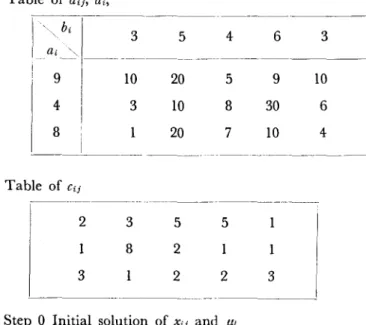
§ 7. A NUMERICAL EXAMPLE OF CAPACITATED HITCHCOCKPROBLEM TREATED AS A MULTI-PARAMETRIC PROGRAMMING Hitchcook problem is n

L:

Xij==ai, j;1 m

L:

Xij=bj, i==l i=l, 2"", rn, j= 1, 2, ... , n, minimize

L:d

i j Xij'

We regard above capacitated Hitchcock problem as the following multi-parametric programming with parameters p" P2, .• " pm

Primal Dual Method of Parametric Programming

P*I,uI, .. " ,um

0;:;;;

Xi};:;;; Cij,

mmlmlze Edij xi}.

Vj~O, Wij~O,

dij+Vj-Ui

+

Wij~O, maximize E,uiUi- ,r.bjvj- ECijWij,

J

135

if we add ,u= fl1

+ ... +

,um, then we have one-parameter programming D*I,u·

7.1. Aprocedure for solving of P*I,uh ···,,um or D*lfll' "',pm is as follows.

a. Fiast of all we put Xij=O jl)r all i, j, Ui=Vj=O and Wij=O, so we have the optimal solution of D*lo, .. ',0, P*lo, .. " o.

b. To solve RP*I,uh .. ',,um and RD*

Vj~O, Wij~O, dij+Vj-Ui+Wij~;:;O, dij + V j-Ui+Wij==O, Wij=O, if Xij>O, if xij<Cij, maximize Ul, 1= l, 2, .. " m.

f

0 if i "'rI, E~L=

1

1 if i=l, J ~L~O, if Xij=O, ;;j;:;;;O, if Xij==Cij,

136 Reijiro Kurata

minimize

L:.;L

di j •

i, j

c. Simultaneous optimal solutions of RP*t for I = l, ... , rn, IS

deter-mined as follows. o

f

0, {jj= I l 00, 2k+J 2k ai

=

min (dij

+

(jj), j(X;j<C;j) 2k+2 2k 2k+l

{jj

= min

{{ji> min (ai -dij)}, i(x;j>O)

00

r

Ui=ai,

l

Vj=~j.

d. Optimal solution of RD*t IS determined as follows. When we

represent Ul in the form

L:

±di,;, if +dij resp. -dij appears in

L:

±diJ, then we put ~L= 1 resp.

';L=

-1, otherwise ~;j=O.

e. Determination of O,'S

We determine 01 under the conditions

m

L:

Ol

L:

.;L:;;,bj,

t=1 i

and 8t~0, making L:Bl as large possible. I

f. To change flows

{-ll change to {-ll+81

Xi.} change to Xij+

L:

';!j 01 I

Primal Dual Method of Parametric Programming 137

Remark 1. As easily seen, L;

i:L=o

or 1 for j such that bj>O,

- J

L; Ol L; ~L~bj are very simple form, but the author is not aware of any

I j

simple algorithm other than simplex method to determine Ol'S.

Remark 2. The Hdtchcock problem can be treated as a

one-para-meter problem P*I,u and D*I,u dealt with in 3.2, by adding another source node 0 and m branches (01), ... , (om) related to it. An optimal solution of RP*I,u is given by Ui and Vj found in C together with Uo= min Ut where

(ai>O)

al=al- L;xij. While that of RD*I,u, .;;:()) is equal to .;;:l. with l for which

j /,1 tJ

UO=Ul. Further, an optimal solution of D*I,u+O is given by Xij+O ~~;). 00

is characterized as the maximal {} satisfying {} L; ~:;) ~bj for j such that

bj>O, and

O~Xij+O ~~;)~Cij.

•

Values of di ,;, Cij in capacitated Hitchcock Problem are given as

follows.

Table of dij, ai,

_ . _

-I

bi 3 5 4 6 3 ai '",- --~---9 10 20 5 9 10 4 3 10 8 30 6 8 20 7 10 4 ____ I _______ ._. _____ ~ __ ~ ____ _ Table of Cij 2 3 5 5 8 2 3 2 2 3 .

138 Reijiro Kurata -~---

----~

PI I

~

.. bj

J

3 5 4 6 3 , - ~ !--~', I I 0 9 0 0 0 0 0 0 4 0 0 0 0 0 0 8 0 0 0 0 0 Step 1.

The case solved as a multi-parametric problem (a) ui=r.±dih ul=dI3,

(b) conditions for (j's

01~5 (j2~ 1 (j3~3 fh:;;'ll,

01~9 02~4 03~8

Cc) determination of 01 and next PI

01=4, O2=1, 03=2 Pl=4, P2=l, P3=2 (d) change of Xi} Xij->Xij+

r.

01 ~W 1 XI3=4, X21 =1, X31=2

Primal Dual Method of Parametric Programming I I ·' _ bj . PI _ ' _ _ I_l!~ __ _ 4 2 Sept 2 5 3 6

o

5

o

2

o

o

o

(a) ul=d14, u2=d25, u3=da5

0---6-'----3---1 I 4

o

o

o

o

o

o

o

o

(b) 01;;;;;6, O2+03;;;;;3 01 ;;;;;:1, O2;;;;;1, 03;;;;;3, (c) 0_{1 =5,} O2=0, 03=3 (d) x14=5, X25=0, X35=3, , " bj

I

0 5 I _PI iii ~--- -- --~----9 0 0 0 3 0 5 3 2 0 Step 3 (a) Ul =dI5 +d31 +d22-d21-d35'

o

-1

o

o

o

o

o

Pl=9, 0 4 0 0

o

o

o

pz = 1, 5 0 0

o

-1 P3=5 0 0 3 3 139

140 _{Reijiro Kurata} (2) t;2ij _i 0 0 0 0 0 0 0 0 0 0 0 0 0 0 _I I ~---. - - - - -(3) t;3ij - ~ - - - -

----~---1

0 0 0 0 0 I -1 0 0 0 _I 0 0 0 0

_I

. _ _ 1

Cb)

81+82+83;;;;5, -81-82;;;;;-1, -81;;;;;-3 81;;;;1, 01+03;;;;1, °1+°2+ 03;;;;8, 81~0, 82~3, 83~3

CC)

_{81=0, 82=3, 03= 1} Pl=9+0=9, P2=1+3=4, P3=5+1 =6

Cd)

XI5=0+0=0, x31=2+1=3, x22=0+3+1=4 X21= 1-1=0, X35=3-0=3. -- - - - ---- ---- - ~ ~ -Pi 0 0 0 iij

_"

9 0 0 0 4 5 0 4 0 0 4 0 0 0 6 2 3 0 0 0 3 - -- - - - -Sept 4

Ca)

ul=d14 , u2=d22, u3=d34

Cb)

O2;;;;1, 83;;;;1, °1;;;;0, 82

;;;;4,

03;;;;2, 81;;;;0, 82;;;;0, 83

;;;;2

Cc)

01=0, 82=0, 83=1, Pl=9, 112=4, P3=7

Primal Dual Method of Parametric Programming , - I -r~- b_j I 'fll _~ I I I a i ' I 1 _ _ _ _ _ _ 1 _ _ _ _ I i I ! 9 0 I _{4 0} 7 Step»

Ca) ul=d12 u2=d22 Cb) (}1 +(}2+(}a~1 (}1 ::;;3, _O2::;;4, Cc) (}1=0, O_2=0, Cd) xa2=0+1=1 fll 9 4 8 Step 1

o

o

o

0 0 0 0 4 0 4 0 3 0 0 ua=da2 Oa::;; 1, 01~0, (}a=l, fll=9, 0 0 0

o

o

3

o

4 4

o

o

0 0 5 0 0 0 3 (}2~0, (}a~l fl2=4, fla=8

o

(}

5

o

o

o

3

The case solved as a single parametric problem Ca) Uo=

L:

±dij, uo=ua=da1

Cb) Oo=maximum (} such that

142 Step 2 9 4 5 Ca) uo=us=dS5 Cb) 00=3

o

o

o

3 Reijiro Kurata -5

o

o

o

4

o

o

o

6

o

o

o

3

o

o

o

Cc) p=3+3=6, xs5=0+3=3 --O---~----~---- --~-~~---I i - - - - ---1 Step 3 9 4 2 Ca) uo=ul=d1S Cb) 00=4

o

o

3

o

o

o

Cc) p=6+4= 10, xls=0+4=4

o

o

o

_ b:

I

0 5 0 ~ai~I _____________ _

o

o

o

6 5 0 0 4 0 4 0 0 0 0

o

I

o

3

o

o

o

-'---_2_-'-- __ 3 _ _ _ 0 _ _ _ 0 _ _ _ 0 _ _ _ 3

~_I

144 Reijiro Kurata Step 7

Ca)

uo=u3=d32

Cb)

00=1

Cc)

p=20+1=21, x32=0+1=1

I~I

0 0 0 0 0 ! ai 0 0 0 4 5 0 0 0 4 0 0 0 0 3 0 3 REFERENCES

[I] E. Kelley, Jr., Parametric programming and the primal dual algorithm, Opns. Res., 7, 327-334 (1959).

[2] L. R. Ford and D. R. Fulkerson, A simple algorithm for finding maximal network flows and an application to the Hitchcock problem, Canadian J. Math., 9, 210-218 (1957).

[3] L. R. Ford & D. R. Fulkerson, A primal-dual algorithm for the capacitated Hitchcock problem, Naval Research Logistic Quarterly, Vol. 4, No. I, 47-54 (1957).

[4] D. R. Fulkerson, A network flow computation for project cost curves, Management Sci., Vol. 7, No. 2, January, 167-178 (1961).

[5] M. !ri, A new method of solving transportation network problems, J. Oper-ations Res. Soc. Japan, Vol. 3, No. I and 2, October, 27-87 (1960).

[6] J. E. Kelley Jr., Critical path planning and sch(duling mathematical basis, Operations Research, Vo. 9, May, 296-320 (1961).