東北大学機関リポジトリTOUR

Transmission Strategy for Intelligent Network

Traffic Control

著者

Mao Bomin

学位授与機関

Tohoku University

学位授与番号

11301甲第18770号

URL

http://hdl.handle.net/10097/00127356

Strategy for Intelligent Network Traffic Control

A dissertation presented

by

Bomin Mao

submitted to

Tohoku University

in partial fulfillment of the requirements

for the degree of

Doctor of Philosophy

Supervisor: Professor Nei Kato

Department of Applied Information Sciences

Graduate School of Information Sciences

Tohoku University

January, 2019

Strategy for Intelligent Network Traffic Control

A dissertation presented by

Bomin Mao

approved as to style and content by

Professor Nei Kato,

Graduate School of Information Sciences

Professor Ayumi Shinohara,

Graduate School of Information Sciences

Professor Masanori Hariyama,

Graduate School of Information Sciences

Associate Professor Zubair Md. Fadlullah,

Graduate School of Information Sciences

Tohoku University

Sendai, Japan.

Recent years, an increasing number of devices are connected to the Internet for pro-viding users with various kinds of services. Accompanying the era of Internet of Things (IoT), the number of devices connected to the Internet will be three times as high as the global population in 2021. To offer users different services, the connected devices generate and receive the traffic. Therefore, the significant increase in the quantity of the connected devices usually leads to the exponential growth of the global IP traffic. It is forecast by the industry that the global IP traffic will increase nearly threefold over the next 5 years and reach 3.3 ZB annually by 2021. The surging traffic demand does not mean the growing profits for the Internet Service Providers (ISPs). On the other hand, the ISPs are confronted with the problem of declining profits due to the traffic explo-sion. This is because the main idea behind the routing algorithms has traditionally been remarkably similar and the manner in which the Internet core and the wired/wireless heterogeneous backbone networks are constructed have largely remained unchanged over the years. To accommodate the tremendous growth of network traffic, the ISPs have to reconsider the core network structure and the packet transmission strategy instead of just adding more/larger routers and more/faster links to scale up the Internet core infrastructure, which on the other hand results in a huge cost.

As we know, the computation capacities of different platforms, such as the Central Processing Unit (CPU) and the Graphic Processing Unit (GPU), are enlarged significantly driving by the Moore’s Law. For example, the single precision processing power of V100 GPU accelerator launched by Nvidia in June 2017 reached as high as 14028 GFLOPS, while that of S870 GPU in May 2007 was only 1382.4 GFLOPS. Besides the much better experience realized by the increasing computation capacities, some existing technologies have benefited from the more powerful computation platforms and achieved some break-through. For instance, as one of the machine learning techniques, the deep neural networks can be trained with much lower time consumption, which lays the solid foundation for the wide applications. Currently, deep learning, emerged from the deep neural networks, has shown its predominant intelligence in many complex activities. Moreover, researchers have also considered this technique to develop the networking management algorithms to improve the performance.

Inspired by the development in the computing hardware and the Artificial Intelligence (AI) technology, in this dissertation, we explore new opportunities in packet process-ing with deep learnprocess-ing to inexpensively shift the computprocess-ing needs from rule-based route computation to deep learning based route estimation for high-throughput packet process-ing. Also, driven by the development of the computation platforms, Software Defined

Moreover, multi-core platforms significantly promote SDRs’ parallel computing capacities, enabling them to adopt artificial intelligent techniques to manage routing paths. This dis-sertation first envisions a supervised deep learning system to construct the routing tables and show how the proposed method can be integrated with programmable routers using both CPUs and GPUs. We demonstrate how our uniquely characterized input and out-put traffic patterns can enhance the route comout-putation of the deep learning based SDRs through both analysis and extensive computer simulations. In particular, the simulation results demonstrate that our proposal outperforms the benchmark method in terms of delay, throughput, and signaling overhead.

Since the labeled data is usually unavailable in some Software Defined Communica-tion Systems (SDCSs) with heterogeneous networks as the data plane, the supervised training manner is not suitable. To alleviate the congestion in the SDCSs with varying traffic patterns, in this dissertation, we utilize Convolutional Neural Networks (CNNs) to intelligently compute the paths according to the input real-time traffic traces. To reduce the computation overhead of the central controller and improve the adaptation of CNNs to the changing traffic pattern, we consider an online training manner. Analysis shows that the computation complexity can be significantly reduced through the online training manner. Moreover, the simulation results demonstrate that our proposed CNNs are able to compute the appropriate paths combinations with high accuracy. Furthermore, the adopted periodical retraining enables the deep learning structures to adapt to the traffic changes.

The above research focuses on the static network scenarios. However, it has been forecast that the traffic generated by the wireless and mobile devices will jump to more than 63% of the global IP traffic by 2021. Therefore, we further propose a Value Iteration Architecture based Deep Learning (VIADL) method to conduct routing design in order to address the limitations of existing deep learning based routing algorithms in dynamic networks. Besides the network performance analysis, this dissertation also studies the complexity of our proposal as well as the resource consumption in different deployment manners. Moreover, this dissertation adopts the Heterogeneous Computing Platform (HCP) to conduct the training and running of the proposed VIADL since the theoretical analysis demonstrates the significant reduction of the time complexity with the multiple GPUs in HCPs. Furthermore, simulation results demonstrate that compared with the existing deep learning based method, our proposal can guarantee more stable network performance when network topology changes.

Firstly, this dissertation would have never been completed without the continuous support and guidance from my supervisor, Prof. Nei Kato. I have been really fortunate to have him as my supervisor since he provided me enough freedom and resource to conduct the research I feel interested in. His kindness, prudence, and work of ethics have made my PhD period one of the best periods of my life. I am also grateful to Associate Prof. Zubair Md. Fadlullah for closely watching, directing, and guiding me throughout each stage of this work. His enthusiasm and prompt suggestion always inspire me to work hard towards my goal. I could not find works strong enough to express my gratitude for him. I would like to thank also the other two professors in my thesis committee, Prof. Ayumi Shinohara and Prof. Masanori Harayama, for their interest, concern, and valuable comments on both the writing of the thesis and the defense.

During the three and half years’ study overseas, I always feel fortunate to meet my wife, Ms. Wei Zou. She has offered me so much support which enables me to concentrate on my research. Being accompanied by her, to study overseas becomes more meaningful and interesting. I wish to thank my dear parents who were always supporting and encouraging me to strict on my choice. I am deeply grateful for their strong faith in me. I cannot imagine how much hardships they have gone through to bring up me, my brother and sister. I would also link to sincerely thank my brother and sister for that they take my responsibility to look after my parents when I was studying overseas. I would repay them during my rest life.

This dissertation would not be possible without the help of my colleagues and friend, Fengxiao Tang. I would never forget his valuable suggestions, discussions, and help over the years. Special thanks go to Motoko Shiraishi, Keisuke Miyanabe, and Yibo Zhou for sincerely helping me with all the necessary documents. Acknowledgments are also given to Chinese Scholarship Council (CSC) for the strong support that enabled me to pursue the challenging route during my doctoral years. Last, but not least, special thanks to all of my lab-mates for their responsiveness, technical help, and mainly for having contributed to this long journey I had to make to pursue my Ph.D degree.

Abstract i

Acknowledgments iii

1 Introduction 1

1.1 Background . . . 1

1.2 Breakthrough of Deep Learning . . . 3

1.3 Development of Hardware Computation Capacities . . . 4

1.4 Purpose of Research . . . 6

1.5 Summary and Organization of the Thesis . . . 8

2 Overview of Deep Learning and Traffic Control 10 2.1 Introduction . . . 10

2.2 Overview of Deep Learning Technologies . . . 10

2.2.1 Preliminaries of Deep Learning . . . 12

2.2.2 Two Commonly Utilized Deep Learning Architectures . . . 15

2.2.2.1 Deep Belief Architecture . . . 15

2.2.2.2 Convolutional Neural Networks . . . 19

2.2.3 Different Training Manners . . . 23

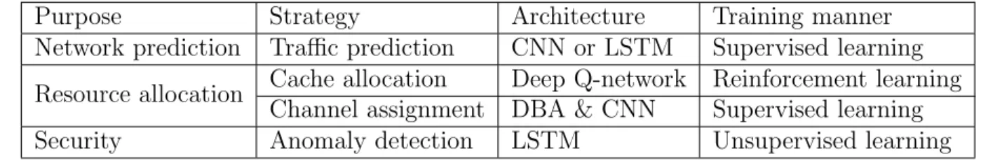
2.2.4 Survey of Deep Learning Based Networking . . . 24

2.2.4.1 Network Parameter Prediction . . . 24

2.2.4.2 Intelligent Resource Allocation . . . 25

2.2.4.3 Smart Anomaly Detection . . . 25

2.3 Overview of Traffic Control . . . 26

2.3.1 Traditional Traffic Control Strategies . . . 26

2.3.1.1 Data Link Layer . . . 27

2.3.1.2 Network Layer . . . 27

2.3.1.3 Transport Layer . . . 28

2.3.2 Research on Deep Learning Based Traffic Control . . . 28

2.3.2.2 Deep Learning Structure Construction . . . 29

2.3.2.3 Network Performance Analysis . . . 29

2.3.2.4 Computation Analysis and Proposal Deployment . . . 30

2.4 Summary . . . 30

3 Deep Learning Based Routing Algorithm for Core Networks Running on GPU Accelerate SDRs 31 3.1 Introduction . . . 31

3.2 Design of Deep Learning based Routing Strategy . . . 32

3.2.1 Input and Output Design . . . 32

3.2.2 Deep Learning Structure Design . . . 34

3.2.3 Considered Router Architecture . . . 35

3.3 The Procedures of the Proposed Deep Learning based Routing Strategy . . 37

3.3.1 Initialization Phase . . . 37

3.3.2 Training Phase . . . 37

3.3.3 Running Phase . . . 39

3.4 Computation Performance Analysis . . . 40

3.4.1 DBA Precision Analysis . . . 41

3.4.2 Complexity Analysis of the Training Phase . . . 42

3.4.3 Complexity Analysis of the Running Phase . . . 45

3.5 Network Performance Evaluation . . . 47

3.6 Summary . . . 51

4 Online Learning Based Routing Strategy for Software Defined Commu-nication Systems 53 4.1 Introduction . . . 53

4.2 Problem Statement and Model Design . . . 55

4.3 Procedures of Our Proposal . . . 58

4.3.1 Initial Phase . . . 58 4.3.2 Running Phase . . . 60 4.3.2.1 Data Collection . . . 60 4.3.2.2 Routing Judgement . . . 61 4.3.2.3 Retraining Phase . . . 62 4.4 Complexity Analysis . . . 63 4.5 Performance Evaluation . . . 64 4.6 Summary . . . 68

5 Value Iteration based Deep Learning Architecture for Routing in

Dy-namic Networks 69

5.1 Introduction . . . 69

5.2 Problem Formulation . . . 70

5.3 Preliminaries . . . 73

5.3.1 Markov Decision Process (MDP) . . . 73

5.3.2 Value Iteration . . . 75

5.4 Design of the Deep Reinforcement Learning Based Routing Strategy . . . . 75

5.5 Complexity Analysis From the HCP Perspective . . . 79

5.6 Performance Evaluation . . . 81

5.6.1 Deployment Analysis . . . 83

5.6.2 Performance with Link Failures . . . 85

5.7 Summary . . . 86

6 Conclusion 87 Appendix 90 Method to Adjust the Weights and Biases of RBMs . . . 90

Bibliography 93

1.1 The Global IP Traffic per Month. . . 2

1.2 The next generation network paradigm. . . 5

1.3 The Nvidia GPU processing power roadmap. . . 6

1.4 Recent inter-disciplinary trends indicate an inter-disciplinary area involving computing systems, computer networks, and machine intelligence. Partic-ularly, network traffic control systems are becoming robust and intelligent owing to the advancement in CPU/GPU technologies and deep learning, respectively. . . 7

1.5 The research contents of this dissertation. . . 8

2.1 The architecture of deep neural networks. . . 11

2.2 The commonly utilized deep learning architectures. . . 12

2.3 Considered model of the proposed deep learning system. . . 15

2.4 The process of convolution between two three-dimensional matrices. . . 20

2.5 The timescales of approaches to congestion control. . . 27

3.1 Considered system model and problem statement. . . 32

3.2 Considered input and output design. . . 33

3.3 The architecture of GPUs and steps of how packets are passed in the GPU-accelerated SDR. . . 35

3.4 Mean Square Errors (MSEs) of different DBAs. . . 40

3.5 The time cost of training phase on the chosen GPU and CPU-based SDRs. 45 3.6 The time cost of running phase on the chosen GPU and CPU-based SDRs. 46 3.7 Comparison of network performance under different network loads in our proposal and the bencmark method (OSPF) in terms of signaling overhead, throughput, and average delay per hop. . . 48

3.8 Comparison of network performance under different signaling intervals in our proposal and the bencmark method (OSPF) in terms of signaling over-head, throughput, and average delay per hop. . . 49

4.2 An illustrative example: when switches S1, S2, and S3 choose S5 as the

next node to destination S8, S5 will be the bottleneck, which means that

traffic congestion will easily happen to S5. . . 55

4.3 The input of the CNN in our proposal. . . 56

4.4 The process in the running phase. . . 62

4.5 The network performance before and after training. . . 65

4.6 The network performance comparison between the conventional routing protocol and our proposal in terms of packet loss rate and average packet delay. . . 65

4.7 The throughput comparison in the considered SDCS. . . 66

4.8 Comparison of SDCS performance under different packet generation rates in our proposal and the bencmark methods (OSPF) in terms of packet loss rate, average packet delay, and throughput. . . 67

5.1 The considered network topology. . . 70

5.2 The Heterogeneous Computing Platform (HCP) and the applications built on it. . . 71

5.3 The proposed Value Iteration Architecture (VIA). . . 76

5.4 The log time cost of training VIA with the single GPU HCP and the multiple GPUs HCP. . . 79

5.5 The log time cost of running VIA with the single GPU HCP and the mul-tiple GPUs HCP. . . 80

5.6 Training computation consumption of networks with different percentages of centralized controlled switches. . . 82

5.7 Running time cost for networks with different percentages of centralized controlled switches. . . 83

2.1 Comparison of three training methodologies. . . 23

2.2 Existing networking research based on deep learning . . . 24

2.3 Some congestion control protocols in the transport layer. . . 28

3.1 Routing Table Built in R3. . . 39

3.2 Effect of different input and output characterization strategies on the net-work control accuracy for N =16. . . 42

4.1 The parameters of the considered CNN structure . . . 63

3G The third Generation of wireless mobile telecommunications technology

4G The forth Generation of wireless mobile telecommunications technology

5G The fifth Generation of wireless mobile telecommunications technology

ADD Addition

AI Artifical Intelligence

AP Access Point

CAIDA Center for Applied Internet Data Analysis

CD Contrastive Divergence

CIFAR Canadian Institute for Advanced Research

CNN Convolutional Neural Network

CPU Central Processing Unit

DBA Deep Belief Architecture

D2D Device to Device

DIV Division

DMA Direct Memory Access

DNN Deep Neural Network

DRAM Dyanmic Random Access Memory

ECN Explicit Congestion Notification

EXP Exponention

HTTP Hyper Text Transfer Protocol

IoT Internet of Things

ISP Internet Service Provider

GB Giga Byte

Gbps Giga byte per second

GHz Giga Hertz

GPU Graphic Processing Unit

HCP Heterogeneous Computing Platform

IEEE Institute of Electrical & Electronics Engineers

IETF Internet Engineering Task Force

IP Internet Protocol

LSTM Long-Short Term Memory network

MDP Markov Decision Process

MSE Mean Square Error

ML Machine Learning

MOS Mean Opinion Score

MUL Multiplication

NAPI Northbound Application Programming Interface

NEG Negation

NIC Network Interface Card

NN Neural Network

OD Origin Destination

OSPF Open Shortest Path First

QoS Quality of Service

RAM Random Access Memory

RBM Restricted Boltzmann Machine

ReLu Rectified Linear Units

SAPI South Application Programming Interface

SDCS Software Defined Communication System

SDN Software Defined Networking

SDR Software Defined Router

SIMD Single Instruction Multiple Data

SM Streaming Multiprocessor

SP Shortest Path

SQRT Square Root Operation

SUB Subtraction

SVM Support Vector Machine

TCP Transmission Control Protocol

V2X Vehicle to Everything

VIA Value Iteration Architecture

VIADL Value Iteration Architecture based Deep Learning

WMN Wireless Mesh Network

WLAN Wireless Local Area Network

XCP eXplicit Control Protocol

Introduction

1.1

Background

In recent decades, it has been witnessed that the significant improvement has been ful-filled in the communication field to provide people with services of better quality and more convenience due to the development of various technologies, such as Fiber-Wireless (FiWi) [1], Device to Device (D2D) [2], and 5G [3]. For example, the emerging mobile telecommunication technology, 5G, can offer people Internet connections with a speed of 1 Gbit/s [4], while 3G proposed in 2000 can only provide an information transfer rate of lower than 1 Mbit/s [5]. Inspired by the development, new Internet services requiring much higher packet transfer rate become a reality. The 5G network can transfer the real-time road information to automatic vehicles in time for avoiding the potential acci-dence [6]. Another more encouraging application is the Internet of Things (IoT), which enables everything to be connected to the Internet [7]. The IoT technology creates op-portunities for more direct integration of the physical world into computer-based systems, resulting in efficiency improvements, economic benefits, and reduced human exertions [8]. On the one hand, the development of communication technologies is beneficial to human being’s life. On the other hand, as more Internet services are emerging, the Internet Service Providers (ISPs) are confronted by several challenges [9]. Recent years, the network traffic is increasing tremendously. The global Internet Protocol (IP) traffic per annum exceeded the ZettaByte (ZB) threshold at the end of 2016, and is expected to increase up to 3.3 ZB by 2021 as shown in Fig. 1.1 [10]. It becomes critically urgent to improve the traffic control performance in order to provide the Internet services of guaranteed quality. At the same time, it is expected that the number of devices connected to the IP networks will be three times as high as the global population in 2020 [10]. As the packets are generated by various devices for different services, the heterogeneous packet configurations as well as the corresponding different requirements for the Quality of Service (QoS) further complicate the problem.

0 0.5 1 1.5 2 2.5 3 3.5 4 2016 2017 2018 2019 2020 2021 An n u al Glob al IP Tr af fic (ZB )

Figure 1.1: The Global IP Traffic per Month.

To accommodate the tremendous growth of network traffic, the Internet core infras-tructure has simply continued to scale up by adding more/larger routers and more/faster links [11]. The increasingly larger core networks have driven the architectures of core routers to be more powerful in computation and switching capacities. Even with the recent surge in the data traffic, the network operators are confronted by the challenges of traffic management for ensuring the QoS as well as dealing with the declining profits [12], which is because the hardware solution results in a massive investment splurge. Besides the implementation of more infrastructure, scholars have conducted a lot of meaningful research on the traffic control algorithms, which can be utilized in specified scenarios for some performance improvement [12, 13]. However, most of these strategies cannot be practically applied, for which two reasons can be summarized. First, current routers and switches still consist of proprietary hardware, meaning that the routing strategies are integrated into the specified hardware to fulfill the packet forwarding tasks. There-fore, the software aspect of traffic management mainly focuses on the application of new routing strategies that may not be possible until a new generation of capable hardware architectures emerge [14]. Second, current packet transmission strategies lack the ability of reconfiguration to fit for the changing network environment. Due to the limitations of fixed hardware architectures, many factors are neglected when designing the algorithms to reduce the computation overhead. Therefore, the current packet transmission strategies still follow the traditional manner (e.g., the Shortest Path (SP) algorithm and so forth) which chooses the paths according to the maximum or minimum metric values [15]. To design an efficient traffic control strategy, it is necessary to improve the packet forwarding algorithms and reconsider the hardware architecture.

1.2

Breakthrough of Deep Learning

Recent years, the field of Artificial Intelligence (AI), dictated by deep learning, is drawing the attentions from the academia and industry. Technology giants such as Google, Mi-crosoft, Facebook, Amazon, Nvidia, and others are investing heavily with their powerful computing resource to drive AI research, particularly aiming at deep learning break-throughs [16]. As the most efficient and promising AI technique, deep learning is now a thriving field with a widely covered active research topics and relevant applications rang-ing from speech recognition to driver-less smart cars [17]. In 2006, a group of researchers brought together by the Canadian Institute for Advanced Research (CIFAR) introduced an unsupervised learning method to pretrain the deep forward neural networks, which enables the hidden layers of deep neural networks to extract the features from the input data without requiring labeled data [18]. Since this method pretrains the neural networks layer by layer with the reconstruction objective, the weights of a deep neural network can be initialized to sensible values, which significantly overcomes the difficulty in training a deep architecture. As the deep architectures can learn more complex features, in March 2016, Google’s DeepMind AI program firstly adopted the deep learning technique in the board game ”Go”, which is concerned with more than 2 × 10170 _{legal positions [19]. And}

the developed programs, AlphaGo and AlphaGo Zero managed to beat the world top players, Lee Sedol and Ke Jie, in October 2015 and May 2017, respectively [19, 20]. The breakthrough of the deep learning technology in board games inspires people to realize its huge potential and also encourages researchers in different fields to develop and discover the intelligent solutions of complex problems. Nowadays, deep learning has been widely studied and applied in the fields of medical diagnose, automatic drive, and industrial control [21, 22, 23].

One important reason for the wide applications of deep learning is because of its flexibility resulting from the various architectures, different training manners, and cor-responding numerous algorithms. For instance, as a machine learning method, the con-structed deep learning architectures can be trained with different manners according to the purpose. Specifically, the supervised learning is usually applied for classification and regression problems, and the unsupervised learning is suitable for clustering, dimension-ality reduction problems, while the reinforcement learning is mainly utilized to learn a policy [24]. To fit for the various application scenarios and purposes, different deep learn-ing architectures have also been developed, such as the Deep Belief Architecture (DBA), Convolutional Neural Network (CNN), Long-Short Term Memory network (LSTM), which significantly increases the flexibility and efficiency of this technique. Therefore, it can be concluded that deep learning is one of the most important paradigm technologies in the future [25].

As mentioned above, the deep learning technique can be utilized to effectively analyze the complex relationships among multiple inputs through training with example data. The trained deep learning architecture can predict the values of some parameters when we input the necessary information. Since the deep learning technique has exhibited superior performance in extremely difficult applications which have traditionally been dominated by humans [19, 20, 25], e.g. board games, it is a promising technology to address the challenges of network traffic control. Moreover, considering the increasing complexities and surging demand in current communication networks, the deep learning technique provides an efficient tool to analyze the network condition and improve the performance. For instance, the deep learning technique can be adopted to accurately predict the traffic changes in heterogeneous networks, which can be considered to improve the packet transmission paths and allocate the network resource, resulting in reduced probabilities of network congestion.

1.3

Development of Hardware Computation

Capaci-ties

Besides the endeavors in software for improving the algorithms, it is also necessary to rethink the core networks. If we want to deploy the deep learning based network traffic control strategies, the network architectures as well as the routers/switches need to be taken into account. As we know, the infrastructures of the Internet backbone networks have remained largely unchanged since the invention [11]. As one of the main components in the core networks, the practically deployed routers still rely on the circuit structure to accomplish the packet switching tasks [26]. Even though the circuit switching can achieve a throughput more than 100 Gbps, the hardware-based architecture lacks flexibility to fit for different routing algorithms, for which the main idea behind the routing algorithms has traditionally been remarkably similar [27]. On the other hand, if we want to apply some new networking algorithms to accommodate the increasing traffic, it is necessary to redesign the hardware architecture of routers and replace existing architecture with the newly developed one, which leads to invaluable expense and time cost.

To address the problems in traditional core network architectures, researchers have proposed the Software Defined Networking (SDN) [28]. Different from the traditional networks which integrate the algorithms into the proprietary hardware architectures to fulfill management in high efficiency, as shown in Fig. 1.2, the proposed SDN consists of three planes: the data plane, control plane, and the application plane, in which the complex network control logics are separated from the data plane to the central con-trollers composed by various computation platforms [29, 30, 31]. Moreover, since they

Internet Router Switch Gateway Server Access point Access point Firewall Northbound APIs

…

Current Network Structure Future Intelligent Software Defined Network Structure

Switch Access point Server Access point

Figure 1.2: The next generation network paradigm.

are based on the general architecture, the SDN controllers allow the upgrade of network management algorithms to be fulfilled by just updating the corresponding applications, which is more flexible than conventional networks [12, 32]. Specifically, any new net-work management application can be installed in the controller through the Northbound Application Programming Interfaces (NAPIs), while the communications between the controller and switches are fulfilled via the Southbound Application Programming Inter-faces (SAPIs) [29, 33]. Due to the advantages in flexibility and simplifications, the SDN technology has been regarded as the next network paradigm as shown in Fig. 1.2 [34]. Moreover, encouraged by the idea of the SDN, researchers have considered the use of software-defined infrastructure which provides the commodity hardware architecture to install the programmable routing strategies to carry out packet processing and transmis-sion, such as the Software Defined Routers (SDRs) [14] and Heterogeneous Computation Platforms (HCPs) [35]. As the critical components of SDNs these software-defined archi-tectures are required not only to support the software-based packet transmission but also to flexibly execute other functions according to the network operators’ needs.

To enable the software-defined architectures to accomplish the complex network man-agement, a general hardware architecture with enough computation capacity is necessary. Therefore, the software-defined architecture integrating modern computation platforms is a promising choice to redesign our backbone networks. As we know, the hardware compu-tation capacity has been significantly improved driven by the Moore’s Law [36]. Fig. 1.3 gives the processing power roadmap of Nvidia’s Graph Processing Units (GPUs), which clearly shows the step-by-step improvement of the computation capacity. The

improve-0.5 1 2 4 8 16 32 2008 2010 2012 2014 2016 Tesla Fermi Kepler Maxwell Volta Double pr eci sion Gf lop s pe r w at t

Figure 1.3: The Nvidia GPU processing power roadmap.

ment makes it possible to consider the commodity hardware for manufacturing network infrastructure. Moreover, to improve the processing throughput performance compara-ble to that of the proprietary-hardware-based routers, researchers as well as networking manufacturers have explored multi-core-based architectures which consist of the Central Processing Units (CPUs) and Graphics Processing Units (GPUs). As we know, the GPUs can execute the same program to process different sets of data in a parallel fashion, while the CPUs undertakes different instructions at the same time [37]. The cooperation of GPUs and CPUs can significantly promote the efficiency to conduct the network manage-ment work. Therefore, the software-defined architectures can be regarded as a competent candidate for conducting the deep learning based routing strategies in modern backbone networks.

The improvement of network architectures and the hardware computation capacities enables the routers/switches to forward packets more efficiently [26]. Also, the general hardware architectures driven by the GPUs pave the way to adopt deep learning in net-working field. Different from conventional traffic control methods which neglect many factors to reduce the analyze complexities, once the computing requirement is satisfied, the deep learning technique enables researchers to take more parameters into account for improving the calculation accuracy. Furthermore, the rich computation resource allows the researchers to learn the traffic control strategies from past network traces through the deep learning technique, which significantly overcomes the difficulty in analyzing the exact relationship among multiple parameters.

1.4

Purpose of Research

After introducing the increasing traffic overhead in current networks as well as the devel-opment in the deep learning and hardware, it is expected that the future network traffic

Deep learning Traffic control systems CPU/GPU architectures Machine intelligence

Figure 1.4: Recent inter-disciplinary trends indicate an inter-disciplinary area involving computing systems, computer networks, and machine intelligence. Particularly, network traffic control systems are becoming robust and intelligent owing to the advancement in CPU/GPU technologies and deep learning, respectively.

control will be an integration of the state-of-art techniques in the communication, com-puter, and computing fields as shown in Fig. 1.4. However, in this paper, we will still survey the existing traffic control methods to analyze the shortcomings. And inspired by the advantages of deep learning as well as the development of computation capacities, we will attempt to adopt the emerging techniques to improve the traffic control performance. Even though various algorithms based on deep learning to optimize the network perfor-mance have been proposed, these approaches do not focus on the network traffic control. In this dissertation, we will focus on the challenges of network traffic control as shown in Fig. 1.5 and extend our research from the following four fields.

Firstly, in this paper, to address the increasing traffic overhead, the existing traffic control strategies need to be studied and analyzed. Since the traffic control needs to be cooperatively fulfilled by different layers, in this paper, we need to do some analysis about the promising directions. Also, the deep learning technique should be discussed since this topic is still new in the networking field. The functions and characteristics of different training manners and architectures need to be studied so as to choose the best one to improve the accuracy and reduce the computation overhead.

Secondly, most of existing research simply utilizes the supervised learning to train a neural network for future predictions, which does not carefully consider the network characteristics. As the input and output of the deep learning architectures impact on the structure design and the prediction accuracy, the characterizations of input and output should be decided according to the considered factors. The purpose of my research is to analyze the factors deeply concerned with the routing decision of core networks and characterize the input and output.

1. Global IP traffic is increasing exponentially;

2. Existing routing protocols cannot cope with complex traffic environment; 3. Current core network structure lacks the flexibilities.

Challenges

Research Contents

1. Utilize deep learning to improve the traffic control performance;

2. Analyze the characterization of the input and output of the deep learning architecture; 3. Consider the design of deep learning architectures for static and dynamic network scenarios; 4. Analyze the deployment of the proposed strategies.

Figure 1.5: The research contents of this dissertation.

The third problem is that most of existing deep learning based research just focuses on static network topology and the trained architectures cannot be applied in a different network scenario. Once the network topology changes, such as some links fail, the trained architectures have to be retrained with new data, which consumes a lot of computation resource and causes some delay. On the other hand, if we do not retrain the deep learning architectures when network changes, the prediction accuracy decreases sharply, losing the advantages of deep learning. In this dissertation, we consider different network scenarios and analyze how to design the intelligent routing algorithms to improve the traffic control for both static and dynamic network scenarios.

Furthermore, current research focuses on the design of algorithms and neglects analysis of the computation resource consumption. Since the deep learning methods are concerned with more computation overhead compared with traditional strategies, our research also discusses the computation consumption. Moreover, the adopted hardware architecture significantly impacts on the computation complexity, while the deployment is a critical problem for the practical application of the proposed deep learning based traffic control methods. Therefore, in this paper, the adopted hardware architectures and the deploy-ment to efficiently conduct the deep learning based methods are also analyzed considering the requirement of the deep learning architecture and the characteristics of network struc-tures.

1.5

Summary and Organization of the Thesis

To explore the deep learning technique to alleviate the increasing network traffic overhead, in this dissertation, we attempt to develop the intelligent packet transmission strategies. We first discuss the main challenges for the Internet networks and survey the existing research to tackle these challenges. The new emerging technique, deep learning, is also introduced. In this part, besides introducing the preliminary knowledge, we focus on some commonly adopted deep learning architectures and the existing intelligent approaches. Based on these introductions, we explain our proposals for different network scenarios.

The remainder of this paper consists of five chapters.

Chapter 2 mainly includes two parts. Firstly, the deep learning technique is in-troduced in this part. The preliminaries of deep learning are explained, including the forward and backward propagations. Then, the three training manners as well as several deep learning architectures are discussed. Moreover, we survey some existing deep learn-ing based research in the networklearn-ing field. Secondly, we analyze the global network traffic burden and the conventional strategies to alleviate the overhead. Specifically, the char-acteristics of heterogeneity and complexities of current networks are emphasized, which leads to extreme difficulties in designing the traffic control algorithms. Considering the promising application of deep learning, we discuss the research contents to adopt the deep learning to design the packet transmission strategy for improving the traffic control. A summary of this chapter is finally given.

Chapter 3 proposes a deep learning based routing strategy for the static backbone networks. In this chapter, we analyze the characterizations of the input and output for constructing the deep learning architectures to improve the traffic control performance. The DBAs are utilized to predict the next nodes and a corresponding path construction strategy is proposed in this chapter. To run the intelligent routing strategy efficiently, we consider the GPU accelerated router architecture and give detailed analysis of the packet processing steps. Simulations also evaluate the improvement in terms of the computation efficiency and network performance.

Chapter 4 proposes an online learning based routing strategy for the considered Soft-ware Defined Communication System (SDCS). Since the traffic pattern in some network keeps varying, the trained deep learning architecture are not fit for the changed surround-ing. Also, it is impossible to collect enough training data to cover all the potential traffic patterns for supervised learning. To tackle this problem, we consider collecting the real-time traffic trace to perodically retrain the utilized CNNs periodically. Then, we conduct the simulations to evaluate the performance.

Chapter 5 studies the deep learning based routing algorithms for dynamic network topology. To address the limitations that most of the adopted deep learning architectures are related to the network topology, we attempt to utilize the deep reinforcement learning method to learn the routing policy beyond the network shape. We consider the Value Iteration Architecture (VIA) to predict the next node with the network topology and the Origin-Destination (OD) information as the input. The HCP is utilized to run the pro-posed intelligent routing method. We evaluate the network and computation performance through simulations.

Chapter 6 finally concludes the thesis. The network performance improvement brought by the deep learning technique is summarized in this chapter.

Overview of Deep Learning and

Traffic Control

2.1

Introduction

As we mentioned in the Chapter 1, the global networks are confronted by increasing traffic overhead and growing complexity. Since it has been illustrated the superiority over human beings in complex activities, such as the games, image classification, and speech recognition, the technology of deep learning is promising to alleviate the traffic overhead. Before discussing the proposed deep learning based traffic control strategies, it is necessary to introduce some preliminaries of this new technique. We will study the mainly concerned calculations as well as the three training manners. After that, several commonly utilized deep learning architectures are discussed, of which the related applications in the networking field are explained to evaluate the advantages of deep learning in performance optimization. Since our purpose is to address the traffic control challenge, we will also survey the traditional strategies in different layers. Then, we analyze the research contents of adopting the emerging AI technology to alleviate the traffic challenge in current networks.

2.2

Overview of Deep Learning Technologies

As one of the most important and basic machine learning architecture, neural networks are one of the most beautiful programming paradigm ever invented to solve complex problems via data analysis. However, this method has not aroused so much attention compared with other machine learning strategies [38], such as Support Vector Machine (SVM) [39], for more than 20 years. Unitl 2006, a Canadian research team improved the training method, which significantly increased the prediction accuracy of neural networks [17].

Input Layer Output Layer Traffic Patterns Packet Loss Link Failure Security time #inbound pac ket s t t+ t+3  t+2 Source Destination Destination Source #i nbo und pac ket s time t+4t+5t+6  Next Node Whole Path Traffic Prediction Initialization Forward Propagation Fine-tuning Backward Propagation 𝑋 𝑌 𝑤

Figure 2.1: The architecture of deep neural networks.

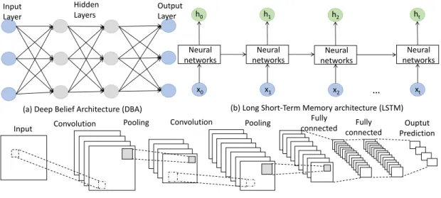
Therefore, it became practical to deploy a large scale of neural networks, referred as deep learning, resulting in the high efficiency in solving complex problems. Fig. 2.1 shows the architecture of deep neural networks, which can be regarded as the most basic deep learning structure [40]. It can be found that it is composed by the input layer, the output layer, and multiple hidden layers. Each layer consists of several units, and each unit is connected to all the units in the adjacent layers through weighted links. If we input some values to the first layer, we can obtain the output through the layer-by-layer propagation of the deep neural networks. The meaning of the output is defined according to our purpose, which can be the values of some predictable parameters, or binary values for classification purpose, or the possibilities of different policies. And the output values are not only dependent on the input layer, but also impacted by the weighted links and the hidden layers. Therefore, we can conclude that the deep neural network represents the relationship between the input and output and the architecture is re-configurable through adjusting the weighted links and hidden layers.

To adopt the deep neural network for definite problems, we first need to characterize the input and output according to our considered scenario and purpose. For example, if the deep learning is utilized to judge whether the network will be congested or not in the next time interval, then the input can be current network traffic patterns, while the output can consist of binary units, of which 1 represents yes and 0 denotes not. Since the characterizations of input and output as shown in Fig. 2.1 impact on the prediction accuracy as well as the design of other layers, it is one of the most important steps for the application of deep learning [41]. As we mentioned in the last paragraph, the architecture of the deep neural network represents the relationship between the input and output, how to adjust the weighted links and hidden layers is vitally critical for the final performance. Moreover, beneficial from the widely meaningful research from the academia and industry,

Hidden Layers Output Layer Input Layer

(a) Deep Belief Architecture (DBA)

Input Convolution Pooling Convolution

Fully

connected _connectedFully Ouptut Prediction Pooling

(c) Convolutional Neural Network (CNN) Neural networks x0 h0 Neural networks x1 h1 Neural networks x2 h2 Neural networks xt ht …

(b) Long Short-Term Memory architecture (LSTM)

Figure 2.2: The commonly utilized deep learning architectures.

scholars have constructed various deep learning architectures, such as the DBA, LSTM, and CNN as shown in Fig. 2.2, to address different scenarios and problems. Since a suitable deep learning architecture can improve the prediction accuracy and reduce the computation overhead, it also needs to be carefully considered when applying this new technique. Furthermore, similar to other machine learning methods, the deep learning architectures can be trained with the manners of supervised/unsupervised/reinforcement learning with different data formats [42]. And the three training manners can be adopted for different purposes. For example, the unsupervised learning is usually adopted for classification, while the supervised learning can be applied to predict the values of some parameters. This section will be expanded from these aspects.

2.2.1

Preliminaries of Deep Learning

Before applying the deep learning technique in our research, we need to know how it works. Since the calculation process varies from architectures, we focus on the most common steps. We still choose the deep neural network as shown in 2.1 as an example. For describing the computations more clearly, we choose two adjacent layers, the (l − 1 )th and lth _{layers as an example. And l}th _{has n}(l) _{units, denoted as U}(l ) _{= {u}

i|i = 1 , 2 , · · · , n(l )}.

Therefore, for the first layer, X = U(1 )_{, while Y = U}(L) _{for the final output layer, if we}

assume the deep neural network has L layers. For each two adjacent layers, the units satisfy the following relationship [40]:

u(l)_j = f (

i=n(l−1)

X

i=1

where w_ij(l ) represents the weight of the link connecting the units u_i(l −1 ) and u_j(l ). b_j(l ) is the bias of unit u_j(l ). f (x ) is the activation function. It can be found that to get the values of units in lth _{layer, we usually utilize a transfer function to activate the sum of}

the weighted units in the (l − 1)th _{layer. And the most popular activation functions are}

given as follows [43]: Sigmoid : f (x) = 1 1 + exp(−x), (2.2) T anh : f (x) = 1 − exp(−2x) 1 + exp(−2x), (2.3) ReLu : f (x) = max(0, x). (2.4)

It can be found that if we know the values of input layer and initialize the weights and biases, we can calculate the units layer by layer, of which the process is usually called the forward propagation as shown in Fig 2.1. Here, note that the methods to initialize the values of weights and biases can be referred to [44]. After obtaining the predicted output denoted as Y0 (Y0 = U(L)_{), we can define a loss function to measure how good a}

prediction model is and the function can be minimized to optimize the prediction. And for the given input X, since the value of the loss function is related to the weights and biases, it can be denoted as C(W, B), where W and B are the weight matrix and bias matrix, respectively. The process to minimize the value of the loss function is termed the training. A most commonly used method of finding the minimum point of C(W, B) is ”gradient descent”. Moreover, to define a loss function depends on a number of factors, such as the presence of outliers, choice of machine learning algorithm, time efficiency of gradient descent, ease of finding the derivatives and confidence of prediction [45]. We can utilize the supervised learning as an example to define the loss function. As we mentioned earlier, the training data of the supervised learning is labeled, denoted as (X, Y ). And the purpose of training in supervised learning manner is to adjust the weights and biases to minimize the distance between the predicted output Y0 and given output Y . Then, the loss function for the supervised learning can be denoted as below:

C(W, B) = Pi=N i=1 (Yi− Y 0 i)2 N . (2.5)

N denotes the number of training data.

To minimize C(W, B), we apply the gradient descent method to adjust the values of weights and biases. We use Equations 2.6 and 2.7 to explain the key ideas.

w_ij(l):= w_ij(l)− η∂C(W, B)

b(l)_j := b(l)_j − η∂C(W, B)

∂b(l)_j , (2.7)

where η is the learning rate which can be adjusted to balance the convergence speed and prediction accuracy. Be repeatedly applying the update rule, we can hopefully find a minimum value of the cost function. However, since C(W, B) is a complex function of the weights and biases, the problem is how to calculate the values of ∂C(W,B)

∂w(l)_ij and

∂C(W,B) ∂b(l)_j .

To solve this problem, we need to analyze the propagation process of the errors in the deep neural networks. We utilize δ to denote the error, then we can obtain the following equation [46].

δ(l)_j = ∂C

∂z(l)_j , (2.8)

where z_j(l) represents the unit’s value before activation in the deep neural networks and can be calculated according to the following equation:

z_j(l)=

nl−1 X

i=1

w_ij(l)u(l−1)_i + b(l)_j . (2.9)

According to chain rule described in Equation 2.9, we can rewrite the Equation 2.8 as below: δ_i(l) = ∂C ∂z_i(l) = X j ∂C ∂z_j(l+1) ∂z_j(l+1) ∂u(l)_i ∂u(l)_i ∂z_i(l) = X j δ_j(l+1)w(l+1)_ij f0(z(l)_i ), (2.10)

From Equation 2.10, it can be found that the error can be calculated from the back layer to the front layer, which is usually call the back propagation as shown in Fig. 2.1. After obtaining the unit error of each layer, we can deduce the partial differential values of weights and biases as shown in Equation 2.11 and 2.12.

∂C ∂w_ij(l) = ∂C ∂z_j(l) ∂z_j(l) ∂w_ij(l) = δ (l) j ∂(w_ij(l)u(l−1)_i + b(l)_j ) ∂w(l)_ij = u (l−1) i δ (l) j (2.11) ∂C ∂b(l)_j = ∂C ∂z_j(l) ∂z_j(l) ∂b(l)_j = δ(l)_j ∂(w (l) ij a (l−1) i + b (l) j ) ∂b(l)_j = δ_j(l) (2.12)

The training process can be conducted by using Equations 2.11 and 2.12 to repeatedly update the weights and biases according to Equations 2.6 and 2.7 till the value of cost function converges. In this way, we can optimize the prediction accuracy of the deep neural networks.

2.2.2

Two Commonly Utilized Deep Learning Architectures

(a) Considered L-layers DBA.

… … … … bias unit visible layer 𝑉 𝑎𝑖 hidden layer 𝐻 𝑤𝑖𝑗 𝑏𝑗

unit j in the hidden layer, ℎ𝑗

unit i in the visible layer, 𝑣𝑖

(b) RBM … … … … … … visible layer hidden layer 𝐻 𝑉 _{Output Layer}𝑌 bias unit j in the hidden layer, ℎ𝑗

unit i, 𝑣𝑖 unit k in the output layer, 𝑦𝑘 𝑎𝑖 𝑐𝑘 𝑏𝑗 𝑤𝑘𝑗 𝑤𝑖j (c) Last RBM.

Figure 2.3: Considered model of the proposed deep learning system.

2.2.2.1 Deep Belief Architecture

The DBA is one of the most commonly utilized deep learning models as shown in Fig. 2.3a. As shown in the figure, we assume the DBA consists of L layers, the input layer, X, the output layer, Y , and the (L − 2) hidden layers. And the DBA can be also seen as a stack of (L − 2) Restricted Boltzmann Machines (RBMs) and a logistic regression layer as the top layer [18]. The structure of each RBM is shown in Fig. 2.3b. It can be seen that each RBM consists of two layers, the visible layer, V , and the hidden layer, H. The units in the two layers are connected through weighted links while those in the same layer are not connected. It should be noted that a weighted bias is given to each unit in both layers. The term wij denotes the weight of the link connecting the unit i in the

visible layer and the unit j in the hidden layer. Also, ai and bj represent the bias of unit

i in the visible layer and that of unit j in the hidden layer, respectively. The learned units’ activated values in the hidden layer are used as the “visible data” for the upper RBM in the DBA. As we mentioned in Sec. 2.2, researchers made great breakthrough in training the deep learning architectures. And according to the research work [18], the deep learning training process consists of two steps: the Greedy Layer-Wise training to initialize the structure and the backward propagation process to fine-tune the structure. For a DBA, the initial process is to train every RBM which is an unsupervised learning process for the reason that an RBM is an undirected graphical model where the units in the visible layer are connected to stochastic hidden units using symmetrically weighted connections as depicted in Fig. 2.3b [18]. While training an RBM, sets of unlabeled data are given to the visible layer, and the values of the weights and biases are repeatedly adjusted until the hidden layer can reconstruct the visible layer. Therefore, the hidden layer after training can be seen as the abstract features of the visible layer. Training an RBM is the process to minimize the reconstruction error with the hidden layer. To mathematically model the training process, we use a log-likelihood function of the visible layer given as follows. Then, the training process is to update the values of weights and biases to maximize the value of the log-likelihood function.

l(Θ, A) =

N

X

t=1

log p(V(t)), (2.13)

where Θ denotes the vector consisting of all the values of the weights and biases of the hidden layer. Θ can be written as Θ = (W, B). W and B represent the vectors consisting of all the weights, wij, and biases of the hidden units, bj, respectively. If we use θ to

denote the unit in Θ, then θ can be any w or b. A consists of the biases of the visible units, ai. N denotes the number of training data. V(t) is the tth training data, probability

of which is p(V(t)_).

To maximize l(Θ, a), we can use the gradient descent of l(Θ, A) to adjust W , A, and B, which can be described as in Equations 2.14 and 2.15.

θi := θi+ η ∂l(Θ, a) ∂θi , (2.14) ai := ai+ η ∂l(Θ, a) ∂ai , (2.15)

where η is the learning rate in deep learning.

To calculate the value of p(V ) (representing any p(V(t))), we need to model the RBM as an energy model since the RBM is a particular form of log-linear Markov Random Field (MRF) [25]. The energy function, E(V, H), and the joint probability function, p(V, H),

are defined as follows. E(V, H) = −X i aivi− X j bjhj− X i X j hjwijvi _(2.16) p(V, H) = e −E(V,H) P V P He−E(V,H) (2.17)

where vi and hj are the unit i in the visible layer and the unit j in the hidden layer

shown in Fig. 2.3b, respectively. Also, the relationship between p(V ) and p(V, H) can be expressed as follows.

p(V ) =X

H

p(V, H) (2.18)

We can use Equations 2.13 to 2.18 to obtain the values of θ [18]. However, the complexity of the calculation of P

V

P

H in Equation 2.17 is 2nV+nH, which is extremely

high (nV and nH represent the dimensions of vectors V and H, respectively). Another

problem is that to calculate Equation 2.17, it is necessary but impossible to consider all the possible values of V and H instead of only the obtained training data. To solve these problems, Hinton et al. proposed the Contrastive Divergence (CD) method [47]. The main idea of CD is to use the Gibbs Sampling method to sample the values of V and H to approximate the real values since the conditional distribution probability of one layer (while the value of the other layer is given), e.g., p(V |H; Θ, A), can be calculated. The detailed procedures of CD is given in the Appendix 6 [47]. As the value of every unit is independent on the other units in the same layer, when one layer is fixed, the conditional distribution probability of the other layer can be calculated as follows,

p(V |H; Θ, A) =Y i p(vi|H; Θ, A), (2.19) p(H|V ; Θ, A) =Y j p(hj|V ; Θ, A), (2.20)

where p(V |H; Θ, A) and p(H|V ; Θ, A) are the conditional probability of V given H and the conditional probability of H given V , respectively. p(vi|H; Θ, A) is the conditional

probability distribution of unit i in the visible layer when the hidden layer is fixed. Also, p(hj|V ; Θ, A) is the conditional probability distribution of the unit j in the hidden layer

when the visible layer is fixed.

p(vi = 1|H; Θ, A) and p(hj = 1|V ; Θ, A) are given as follows. p(vi = 1|H; Θ, A) = f ( X j wijhj + ai) (2.21) p(hj = 1|V ; Θ, A) = f ( X i wijvi+ bj) (2.22)

where f (x) represents the activation activation function.

Since the values of the DBA’s input units representing the numbers of inbound packets are continuous and affected by many factors, we use the Gaussian probability distribution to model the traffic patterns [48]. Therefore, for RBM1 in our proposed DBA,

Equa-tion 2.16 and EquaEqua-tion 2.21 should be revised as follows.

E(V, H) = −X i (vi− ai)2 2σ2 i −X j bjhj− X i X j vi σi hjwij, (2.23) p(vi|H; Θ, A) = N (ai+ σi X j hjwij, σ2i), (2.24)

where σi is the value of the variance for the unit vi. N (ai+ σiP_jhjwij, σi2) denotes the

Gaussian distribution with mean (ai+ σi

P

jhjwij) and variance σi.

The forward propagation follows the above-mentioned equations for the DBA. How-ever, if the DBA is trained with the supervised learning manner, since the output layer has a given label, the last RBM, RBML−2, consists of three layers as shown in Fig. 2.3c [49].

Therefore, the visible layer of RBML−2 consists of not only RBML−3’s hidden layer but

also the output layer of the DBA, Y . And its hidden layer is the top hidden layer of the DBA. The structure of RBML−2is shown in Fig. 2.3c and its energy function is expressed

as follows. To keep consistent with the other RBMs, we use V and H to denote RBML−3’s

hidden layer and the top hidden layer, respectively.

E(V, H, Y ) = −X i aivi− X j bjhj − X k ckyk− X i X j hjwijvi− X j X k hjwkjyk, (2.25)

where Y represents the vector in the output layer. ck is the bias of the unit yk. wkj

represents the weight of the link connecting the units hj and yk.

of the concatenated vector consisting of V and Y is, p(V, Y |H; Θ, A) = p(V |H; Θ, A)p(y|H; Θ, A) =Y i p(vi|H; Θ, A) Y k p(yk|H; Θ, A) (2.26)

We use the method mentioned above to train each RBM. The value of the visible layer of the first RBM is X in the given training data. And after training each RBM, the learned activated value of its hidden layer is used as the “data” for the next RBM in the DBA. Here, it can be found that we train one hidden layer of the DBA at one time via training an RBM. In this way, the DBA gets initialized and the value of Θ is nearly optimum. Then the method of backward propagation described in Sec. 2.2.1 is utilized to fine-tune the DBA.

2.2.2.2 Convolutional Neural Networks

CNNs have achieved the most wide applications in many fields, to name a few, pattern recognition, image processing, video analysis, and natural language processing [17]. As shown in Fig. 2.2c, a CNN is composed of several convolutional layers, pooling layers, and fully connected layers [50]. Different from the Deep Neural Network (DNN), the units in the convolutional layer are just connected to part of the units in next layer, which can significantly reduce the number of parameters. The pooling operation is usually located in-between two successive convolutional layers. In the pooling operation, the result of the convolution operation is sampled to progressively reduce the feature size [51].

Fig. 2.2c depicts the structure of a CNN, which mainly consists of three parts: convolu-tional layers, pooling layers, and fully connected layers. For the purpose of classification, a softmax regression process is usually conducted on the output of the last fully connected layer to get the final output [52, 53]. In the remainder of this section, we will give a detailed introduction on the mathematical formulation of each of these layers.

To describe the calculations more clearly, we consider two layers labeled as the (l − 1 )th and lth layers as an example to explain every operation. The input and output of the convolution and pooling operations are usually represented by a three dimensional matrix, while those of the fully connected layers and softmax operation are denoted as vectors. Moreover, as an activation operation exists in most layers of the CNNs, we adopt Z and U to denote the values of each layer before and after activation, respectively.

For the convolution operation, it is reasonable to assume that the dimension of U(l1−1) (also Z(l1−1)_{) is P × Q × R. Since the CNNs are usually utilized in the image recognition} field, we can consider the three dimensions of the input matrix to denote an image’s height, width, and depth, denoted by P, Q, R, respectively [52]. For instance, in the application

a1 _b1 _c1 d1 _e1 _f1 g1 _h1 _i1 12 3 a1 _b1 _c1 d1 _e1 _f1 g1 _h1 _i1 a2 _b2 _c2 d2 _e2 _f2 g2 _h2 _i2 a3 _b3 _c3 d3 _e3 _f3 g3 _h3 _i3 expand A1 _B1 C1 _D1 ∗ _{∗ ∗ ∗} A1 _B1 C1 _D1 A2 _B2 C2 _D2 A3 _B3 C3 _D3 ∑(Ai_ai_+Bi_bi +Ci_di_+Di_ei₎ ∑(Ai_bi_+Bi_ci +Ci_ei_+Di_fi₎ ∑(Ai_di_+Bi_ei +Ci_gi_+Di_hi₎ ∑(Ai_ei_+Bi_fi +Ci_hi_+Di_i1₎ A2_a2_+B2_b2₊ C2_d2_+D2_e2₎ A2_b2_+B2_c2₊ C2_e2_+D2_f2 A2_d2_+B2_e2₊ C2_g2_+D2_h2 A2_e2_+B2_f2₊ C2_h2_+D2_i2 A1_a1_+B1_b1₊ C1_d1_+D1_e1 A1_b1_+B1_c1₊ C1_e1_+D1_f1 A1_d1_+B1_e1₊ C1_g1_+D1_h1 A1_e1_+B1_f1₊ C1_h1_+D1_i1 A3_a3_+B3_b3₊ C3_d3_+D3_e3 A3_b3_+B3_c3₊ C3_e3_+D3_f3 A3_d3_+B3_e3₊ C3_g3_+D3_h3 A3_e3_+B3_f3₊ C3_h3_+D3_i3 expand + + = 2 3 1

Figure 2.4: The process of convolution between two three-dimensional matrices.

of image classification, researchers usually use a 28 × 28 × 3 matrix to denote a picture, in which 28 is the number of pixels in every edge and 3 is the number of basic color channels which are R, G, and B, respectively. As the purpose of the convolution operation is to extract the distinguished features of the input, the parameters (weights and biases) of the convolution operation consist of a set of learnable filters, each of which can be denoted by a P0 × Q0 × R matrix as the depth of each filter should be the same as that of the input volume. Every filter is small spatially, but extends through the full depth of the input volume. During the forward pass, each filter slides across the width and height of the input volume and a convolution operation is conducted between the filter and the area of the input volume covered by the filter which is shown in Fig. 2.4. The convolution result of the input volume and each filter is named as a feature map. If we use W(l1) _to denote the filters and the kth filter is represented by W(l1)

k , the obtained feature map by

the convolution operation can be shown as follows.

z(l1) i,j,k = (Z (l1−1)_{∗ W}(l1) k )(i, j) + w (l1) bk = R X r=1 P0 X p=1 Q0 X q=1 wp,q,ru (l−1) i+p,j+q,r+ w (l1) bk , (2.27) a(l1) i,j,k = f (u (l1) i,j,k), (2.28)

where f (·) is the activation function and u(l1)

i,j,k is the activated value of the unit in the i th

row and jth column of the feature map. Therefore, z(l1)

i,j,k is the value before activation.

w(l1)

bk denotes the bias of the k

th_{filter and is usually a single numeric value. u}(l1−1)

i+p,j+q,dis the

activated value of unit in the (i + p)th_{row and (j + q)}th _{column. The most commonly used}

activation function is the Rectified Linear Unit (ReLU) function given in Equation 2.4. After the convolution operation, the convolutional layer consists of several feature maps. Since the convolution operation between the input volume and each filter results in a feature map, the number of feature maps is equal to that of filters. Moreover, the size of each feature map is dependent on the following factors: the sizes of the input volume and each filter, the stride of each slide, and the number of zero-padding columns or rows. If we use s and t to represent the number of zero-padding and the value of each slide, then the width and height of the feature are as in Equations 2.29 and 2.30. Here, it should be noted that the advantages of zero-padding are two-fold, namely, to sufficiently extract the features located in the edge of the input volume, and make the height and width of each feature map to be integers.

w(l1) f m = (P − P 0 + 2s)/t + 1, (2.29) h(l1) f m = (Q − Q 0 + 2s)/t + 1. (2.30)

To progressively reduce the spatial size of the representation to reduce the amount of parameters and computation, it is common to periodically insert a pooling layer in-between the successive convolutional layers. The pooling layer is the result of the down-sampling of the convolutionle layer. To make the pooling operation learnable, we usually add two scalar parameters and the mathematical expression is shown in Equation 2.31.

Z(l2) _{= β}(l2)_down(U(l2−1)_{) + b}(l2)_{, (2.31)}

U(l2) _{= f (Z}(l2)_{), (2.32)}

where β(l2) _{and b}(l2) _{denote the learnable parameters of the pooling operation. Z}(l2) _and U(l2) _{denote the values of output matrix of the pooling layer before and after activation,} respectively. down represents the operation of downsampling. There are many types of downsampling methods, among which the most popular one is the max pooling, which just keeps the maximum activation value in every square region of the (l2 − 1 )th layer. In

this way, the height and width of the pooling layer are just half of those of the (l2 − 1 )th

layer while their depths are the same.

After several convolutional layers and pooling layers, the size of the input volume can be significantly reduced. Then, the final pooling layer is connected to the fully connected

layer, in which every unit is connected to all units in the previous layer. If we assume the (l3− 1)th and lth3 layers are the pooling layer and fully connected layer, respectively, the

units in these two layers satisfy the following relationship.

z(l3) i = X j u(l3−1) j w (l3) ij + b (l3) i , (2.33) u(l3) i = f (z (l3) i ), (2.34) where z(l3) i and u (l3)

i are the values of unit i in the l3th layer before and after activation,

respectively. As mentioned earlier, the 3-dimensional matrix in the pooling layer needs to be spread into a vector when connected to a fully connected layer. Then, u(l3−1)

j is the

activated value of unit j in the vector. w(l3)

ij is the weight of the connection between unit

i in the lth₃ layer and unit j in the (l3 − 1 )th layer. b (l3)

i is the bias of unit i in the l th 3

layer. If there are multiple fully connected layers, the relationship between any two fully connected layers also satisfies Equations 2.33 and 2.34.

As the CNN is usually used for classification, if we assume that there are t kinds of different results, then we can use a vector consisting of t binary values to represent the result [53]. And in the vector, only one unit must have the value of 1, the order of which represents the result. Therefore, a softmax regression process is necessary to be conducted on the final fully connected layer. The first step of softmax regression is to convert the values of units in the fully connected layer into possibilities of the results according to Equation 2.35. Then if pi is maximum, we can label unit i in the output layer as 1 while

each of the other units is labeled as 0. We can adopt y to denote the order of the unit, which is labeled 1, meaning that the result of the CNN is y.

pi(x) =

ezi P

jezj

, (2.35)

where pi is the possibility of the appearance of result i. And zi is the value of unit i in

the final fully connected layer.

If the CNN is trained in a supervised manner, the purpose of the training is to maximize the possibility of training data, which can be expressed as a loss function as shown in Eq. (2.36) [52]. C(W, B) = − 1 N( N X i=1 k X j=1 1{y = j} log pi(xi)), (2.36)

where W and B represent the weights and biases of the CNN. N is the number of training data. xi is the ith input training data. Here, 1{·} is the indicator function and its values