Chapter 2 Equilibrium locations of upstream
and downstream firms
権利
Copyrights 日本貿易振興機構(ジェトロ)アジア
経済研究所 / Institute of Developing
Economies, Japan External Trade Organization
(IDE-JETRO) http://www.ide.go.jp
journal or
publication title
New Challenges in New Economic Geography
page range
43-82
year
2010-03
Kumagai, Satoru, ed. 2010. New Challenges in New Economic Geography. Chiba: Institute of Developing Economies.
Chapter 2 Equilibrium Locations of Upstream and Downstream
Firms
Toshitaka
GOKAN
$%Abstract
This paper explores the interaction between upstream firms and downstream firms in a two-region general equilibrium model. In many countries, lower tariff rates are set for intermediate manufactured goods and higher tariff rates are set for final manufactured goods. The derived results imply that such settings of tariff rates tend to preserve a symmetric spread of upstream and downstream firms, and continuing tariff reduction may cause core-periphery structures. In the case in which the circular causality between upstream and downstream firms is focused! as agglomeration forces, the present model is fully solved. Thus, we find that (1) the present model displays, at most, three interior steady states, (2) when the asymmetric steady-states exist, they are unstable and (3) location displays hysteresis when the transport costs of intermediate manufactured goods are sufficiently high.
Keywords: Spatial economics, upstream and downstream firms JEL classification: F02, F12, R12, R13
!!!!!!!!!!!!!!!!!!!!!!!!!
*a Researcher, Economic Integration Studies Group, Inter-disciplinary Studies Center, IDE
1. Introduction
The difference in the tariff rates of products may show that each country intends to promote local production. Kumagai and Kuroiwa (2009) examined the average effective applied tariff rate in intra-regional trade in East Asia in 2006. The effective applied rate is the tariff rate which is actually applied to imported goods from East Asian countries, weighted by the import value from each country. In Vietnam, Lao PDR, Thailand and Brunei, the tariff rate on consumption goods is twice the tariff rate on parts and components. In Korea, China, Malaysia, Indonesia, Taiwan, the Philippines and Myanmar, the tariff rate on consumption goods is four times as high as the tariff rate on parts and components. This implies that most countries prefer to maintain higher tariff rates on consumption goods. Furthermore, these tendencies were clear in the automobile industry as well. To clarify the effects of such difference in tariff rates not only on local production but also on the spread of economic activity, a model is needed which includes the transport costs of intermediate goods and the transport costs of final consumption goods.
Only a small number of papers focus on the agglomeration and dispersion of up-stream and downup-stream firms because of the complexity of introducing two types of firms with increasing returns to scale technologies. The pioneering study of Venables (1996) il-lustrated figuers to show the interaction of upstream and downstream firms in a two-region general equilibrium model. Using a two-region general equilibrium model with upstream and downstream firms and focusing on the agglomeration, Amiti (2005) showed the
ten-sion between factors in Heckscher-Ohlin model and new economic geography model. To avoid complexity, Krugman and Venables (1995) developed a two-region general equilib-rium model with one mass of manufactured products used for intermediary and household consumption, examined the emergence of the core-periphery structure, and showed the convergence of real wages between countries with a decrease in the transport cost of the manufacturing sector. To develop a more analytical model, Ottaviano and Robert-Nicoud (2006) developed a fully solvable general equilibrium model with one mass of manufac-tured products. The advance made by Nicoud (2004) and Ottaviano and Robert-Nicoud (2006), respectively, was to show that the same key features are shared by the most prevalent New Economic Geography models, such as Krugman (1991) and Krugman and Venables (1995) and the models in which firms use unskilled workers as variable costs and the rest of the inputs as fixed costs. Although we assume that the intermediate goods are incurred as fixed costs of downstream firms, Ottaviano and Robert-Nicoud (2006) write that to use intermediate goods in fixed costs is ea (not so) special case.f To realize the same merits as Ottaviano and Robert-Nicoud (2006) in their analysis on the instability of two asymmetric steady-states, this chapter extends Ottaviano and Robert-Nicoud (2006) to in-troduce upstream firms and downstream firms in a model. Such an extension allows us to obtain solvable results even when upstream firms produce intermediary goods and down-stream firms produce consumption goods for households in a two-region general equilib-rium model.
The spatial configuration of economic activities is decided by the balance of the ag-glomeration force and dispersion force. The source of agag-glomeration force is forward and backward linkages, which bring the circular causality. In our model, there are two circular causalities: the interaction between upstream firms and downstream firms and the interac-tion between downstream firms and households. However, it is difficult to focus on two circular causalities at once; we set a fixed number of skilled workers and allow these work-ers to earn in the agricultural sector, although such case emerges when the same wage rates in the manufacturing sector and the agricultural sector. As a result, the mechanism of our model changes depending on the supply of skilled workers. When the supply of skilled workers is scarce, all skilled workers are in the manufacturing sector and the wage rates increase. In this extreme case, this scarcity works as a dispersion force. Only the circular causality between downstream firms and households causes industrial agglomeration. In contrast, when the supply of skilled workers is abundant, there are some skilled workers who are not working in the manufacturing sector. Thus, the regional income in a region does not change. As a result, only the circular causality between upstream firms and down-stream firms works. In the followings, only the latter is fully solved.
The remaining portion of this chapter is organized as follows. Section 2 explains the model, which is solved in Section 3. Section 4 examines the Pareto dominant allocation. Section 5 presents the conclusion.
The economic space is composed of two regions, called north and south, which are sym-metric in terms of tastes, technology and endowments. The economy has two sectors: agri-culture (herein referred to as A) and manufacturing (herein referred to as M). The economy is endowed with two factors of production: entrepreneurs (H) and workers (L).
Workers are not inter-regionally mobile, and regions are endowed with equal supplies of the immobile factor, L, thus L = L∗ = Lw/2. Some workers (L) are entrepreneurs (H),
who can be regarded as human capital, and regions are also endowed with equal supplies of entrepreneurs, H, thus H = H∗ = Hw/2. Entrepreneurs are free to choose to utilize their
human capital or not.
Preferences are identical across all workers and are described by the upper tier con-sisting of a Cobb-Douglas ’nest’ of consumption of the agricultural goods and a composite of all manufactured consumption goods,
U = CµCMµC 1−µ A , CM ≡ !" m+m∗ i=0 c1−1/σc i di #1/(1−1/σc) ; 0 < µ < 1 < σc (1)
where Cµ ≡ µµ(1− µ)µ−1 is constant, and CM and CA are, respectively, consumption of
the CES composite of manufactured consumption goods varieties and consumption of A. Furthermore, m and m∗are the mass (number) of north and south varieties in manufactured
consumption goods, µ is the expenditure share in industrial varieties, and σc is the constant
elasticity of substitution between the varieties. The corresponding indirect utility functions for typical northern entrepreneurs and workers are ωH and ω, where
ωH ≡ wH Pcµ , ω ≡ w Pcµ , Pc ≡ (∆c)−1/(σc−1), ∆c = " mw i=0 p1ci−σdi (2)
wH is the northern wage for entrepreneurs and wH is the northern wage for workers.
Expres-sions for the corresponding southern values are isomorphic. Below, isomorphic expresExpres-sions are omitted.
The agricultural good is homogeneous and produced using workers only. The agri-cultural sector uses a constant-returns technology under conditions of perfect competition. The specific cost function is w. Both regions produce an agricultural good. Trade in the homogeneous A good is costless.
The manufacturing firms are under the condition of monopolistic competition and use the increasing returns to scale technology. As for the technology of downstream firms, fixed and marginal input requirements are satisfied by different factors: the marginal cost is incurred in terms of labor only; the fixed cost is incurred in terms of the differentiated varieties of the manufactured intermediate goods. In symbols, the cost function of the typical northern downstream firm l is given by
Cc(cl) = fcPint+ acclw, Pint ≡ ∆−1/(σint int−1); ∆int ≡
" nw
k=0
p1−σint
intk dk (3)
where ac is the marginal labor requirements in downstream firms, and Pintis the upstream
firm’s price index. Trade in industrial goods is subject to iceberg trade costs; a firm wishing to sell one unit of its good in the other region must ship τc ≥ 1 units since τc− 1 units melt
in transit.
As for the technology of upstream firms, the marginal cost is also incurred in terms of labor only, whereas the fixed cost is incurred in terms of one entrepreneur. The cost
function of the typical northern upstream firm j is given by
Cint(qj) = fintwH + waintqj (4)
where qj is the demand for variety j on intermediate goods. Also, aintis the marginal labor
requirements in upstream firms. Trade in industrial goods is subject to iceberg trade costs; a firm wishing to sell one unit of its good in the other region must ship τint≥ 1 units since
τint− 1 units melt in transit.
Because entrepreneurs and workers are free to choose between the agricultural and manufacturing sectors, the wage rates must be the same in the two sectors within each region, provided that the two sectors exist and entrepreneurs work in the two sectors in the given region. Entrepreneurs’ decisions to work as a worker or an entrepreneur are based on the nominal wage difference. The wage gap between them is expressed as ln (wH/w).
Long-run equilibrium wages for entrepreneursf capital satisfy ln (wH/w) = 0, n ∈ (0, ¯H/fint),
ln (wH/w) > 0, n = ¯H/fint, (5)
ln (wH/w) < 0, n = 0.
The flow of upstream firms is expressed as follows: ˙n = n$ ¯H/fint− n % ln&wH w ' , n˙∗ = n∗$ ¯H∗/fint− n∗%ln ! w∗ H w∗ # . (6)
negative. The flow of downstream firms is regulated as follows: ˙ m = m ln ! πc Pintfc # , ˙m∗ = m∗ln ! π∗ c P∗ intfc # (7) where πcand π∗c are operating profits and Pintfcand Pint∗ fc are fixed costs.
3. Instantaneous Equilibrium
The equilibrium taking as a given the spread of manufacturing firms is analyzed.
The agricultural good is costlessly traded between regions and is chosen as the num´eraire, and thus the price of the agricultural good is one. The equalization of the price of the agri-cultural good causes the wage for workers to also be one in both regions.
From utility maximization, northern consumption of a variety j is cj = p−σcj c(µEc/∆cnw),
where Ec = wHH + w(L− H) is northern expenditure for manufactured consumption
goods. From monopolistic competition, mill prices for all upstream firms are as follow:
pc = ac 1− (1/σc) , p∗c = τc ac 1− (1/σc) (8)
where pc and p∗c are the consumer prices for a typical north-made variety in the northern
market and the southern market, respectively. Likewise, northern demand of a variety l of manufactured intermediate goods is ql = pintl(Eint/∆intnw), where Eint = mPintfc is
northern expenditure for manufactured intermediate goods. Mill prices for all downstream firms are as follow:
pint = aint 1− (1/σint) , p∗int = τint aint 1− (1/σint) (9)
where pintand p∗intare the intermediate manufactured goods prices for a typical north-made
variety in the northern market and the southern market, respectively.
Using the demand functions and mill prices, the profit function for downstream firms (Πcand Π∗c) are as follow:
Πc = µ σc ! Ec ∆c + φc E∗ c ∆∗ c # − (∆int)− 1 σint−1 fc, (10) Π∗c = µ σc ! φc Ec ∆c +Ec∗ ∆∗ c # − (∆∗int)− 1 σint−1 fc; (11)
φc ≡ τc1−σc, φint≡ τint1−σint (12)
Ec ≡ w(L − H) + wHH, Ec∗ ≡ w∗(L∗− H∗) + w∗HH∗, (13) ∆c ≡ m ! ac 1− (1/σc) #1−σc + φcm∗ ! ac 1− (1/σc) #1−σc , (14) ∆∗c ≡ φcm ! ac 1− (1/σc) #1−σc + m∗ ! ac 1− (1/σc) #1−σc , (15) ∆int ≡ n ! aint 1− (1/σint) #1−σint + φintn∗ ! aint 1− (1/σint) #1−σint , (16) ∆∗int ≡ φintn ! aint 1− (1/σint) #1−σint + n∗ ! aint 1− (1/σint) #1−σint . (17)
The value of φc and φint, respectively, ranges from φc = 0and φint = 0, with prohibitive
trade costs to φc = 1and φint= 1, with zero trade costs.
Using the demand functions, mill prices, and the zero profit condition of downstream firms, the profit functions for upstream firms (Πintand Π∗int) are expressed as follow:
Πint= µ σintσc ! m ∆int ! Ec ∆c +φcEc∗ ∆∗ c # +m∗φint ∆∗ int ! φcEc ∆c + Ec∗ ∆∗ c ## − wHfint, (18) Π∗int= µ σintσc ! mφint ∆int ! Ec ∆c + φcEc∗ ∆∗ c # + m∗ ∆∗ int ! φcEc ∆c + Ec∗ ∆∗ c ## − wH∗fint. (19)
Therefore, the zero profit condition of upstream firms implies that the nominal wage rates for entrepreneurs are:
wH =
(&B&C− &A&D)(L− H)H∗+ &A(L− H)b + &B(L∗− H∗)b
(&A&D − &B&C)HH∗− b(&AH + &DH∗) + b2
, (20)
w∗H = (&B&C − &A&D)(L∗− H∗)H + &C(L− H)b + &D(L∗− H∗)b (&A&D− &B&C)HH∗− b(&AH + &DH∗) + b2
(21) where b ≡ fintσcσint/µ, &A≡ m ∆int∆c +m∗φintφc ∆∗ int∆c , &B ≡ mφc ∆int∆∗c + m∗φint ∆∗ int∆∗c , &C ≡ mφint ∆int∆c + m∗φc ∆∗ int∆c , &D ≡ mφintφc ∆int∆∗c + m∗ ∆∗ int∆∗c .
We make the usual choice of units for lightening the following analysis. We normal-ize ac to 1 − (1/σc), aintto 1 − (1/σint), fc to one, and fintto one.
4. Equilibrium
4.1. Agglomeration and Dispersion
The equilibrium resulting from the free choice between the agricultural sector and manu-facturing firms is analyzed in ten cases. As Baldwin (2001) used, local stability is evaluated by linearizing (6) and (7) around an equilibrium point ¯m, ¯m∗, ¯n, ¯n∗. The elements of the
Jacobian matrix can be expressed as in Appendix 1. From Hatman-Grobman theorem (see Hartman 1964: 244, Theorem 7.1), which shows that linearization preserves the qualitative
properties of the nonlinear system in the neighborhood of the equilibrium point when no eigenvalue of the Jacobian matrix has real parts equal to zero, equilibrium is stable when the Jacobian matrix has eigenvalues all with negative real parts.
Agglomeration and abundant supply of entrepreneurs
The manufacturing sector is supposed to be concentrated in the north, with n∗ = m∗ = 0.
Since entrepreneurs are abundant, some entrepreneurs are in the agricultural sector in the north. All entrepreneurs in the south are also in the agricultural sector. Thus, the wage rate of entrepreneurs is one in both regions. Setting ¯m∗ = ¯n∗ = H∗ = 0and using (10) and
(20), the zero profit condition of downstream firms and the equality of wage rates between workers and entrepreneurs implies the following number of upstream firms and downstream firms in the core:
m = µ
σc
(2L)σint−1σint b−σint−11 ≡ m1, n = H = 2L
b , (22)
and the operating profits and fixed costs for upstream firms and the wage rate for en-trepreneurs are as follow.
πc = µ σc 2L m, Pint= n −σint−11 , w H = 2L/n− 1 b− 1 . (23)
Because the entrepreneurs are abundant, we have 2L/b < ¯H.
Examining the instance when all eigenvalues are negative in the above setting as in Appendix B.1, we find that the case when all manufacturing firms are in the north under
2L/b < ¯H is a spatial equilibrium under the following condition:
1
2(φc+ 1/φc) < φint
− 1
σint−1. (24)
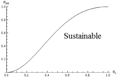
The condition (24) shows the case when downstream firms do not emerge in the periphery. This implies that agglomeration is sustainable whenever transport costs of intermediate goods are high enough and transport costs of final goods are low enough. As explained in Fujita et al. (1999: 249), the right-hand side of the inequality shows the forward linkages between upstream firms and downstream firms. That is, downstream firms need to bear a disadvantage to operate in the region where there are no upstream firms. On the other hand, the left-hand side of the inequality shows the backward linkages between downstream firms and households. The first term in the parenthesis shows that downstream firms have a disadvantage when transporting to the other region, and the second term in the parenthesis shows that transport costs moderate price competition in the periphery.
————————————————————— Insert Figure 1 around here
—————————————————————
To understand the relation with the results of the standard core-periphery model, Figure 1 is helpful. The condition (24) is depicted as a curve in Figure 1. The core-periphery structure is sustainable in the domain under the curve. The diagonal line shows the pair of transport costs when both transport costs take the same value. Supposing that both transport
costs fall along the diagonal line from the origin of Figure 1, the core-periphery pattern becomes stable after transport costs decrease adequately, as discussed in Fujita et al. (1999).
Agglomeration and scarce supply of entrepreneurs
The manufacturing sector is supposed to be concentrated in the north, with n∗ = m∗ = 0.
Since entrepreneurs are scarce, the number of upstream firms is decided by the number of entrepreneurs in the north. All entrepreneurs in the south are in the agricultural sector. Set-ting ¯m∗ = ¯n∗ = H∗ = 0 and using (10) and (20), the zero profit condition of downstream
firms and the scarcity of entrepreneurs implies the following number of upstream firms and downstream firms in the core:
m = µ σc b b− 1(2L− ¯H) ¯H 1 σint−1 ≡ m2, n = ¯H, (25)
and the operating profits and fixed costs for upstream firms, and wage rate for entrepreneurs, are as follows πc = µ σc (2L− ¯H)b (b− 1)m , Pint= n − 1 σint−1, wH = 2L− ¯H (b− 1) ¯H. (26)
Examining the instance when all eigenvalues are negative in the above setting as in Appendix B.2., we find that the case when all manufacturing firms are in the north under 2L/b≥ ¯H is a spatial equilibrium under the following condition:
φint < (b− 1) ¯H 2L− ¯H , (27) and φc[(b + 1)L− b ¯H] + (b− 1)L/φc b(2L− ¯H) < φint − 1 σint−1. (28)
The first condition (27) shows the case when upstream firms do not emerge in the periphery. The right-hand side of (27) is the nominal wage rate of entrepreneurs in the south (the periphery) divided by that of entrepreneurs in the north (the core). That is, upstream firms emerge in the periphery when transport costs are low enough that the decrease in profit caused by the additional transport cost can be covered by the increase in profit due to the relatively lower nominal wage rates of entrepreneurs in the periphery. The second condition (28) is similar to (24). The minor difference in them stems from the asymmetric market size in (28). In Figure 2, (27) is depicted as a horizontal line, whereas (28) is depicted as a curve. As in Figure 1, the diagonal line shows the pairs of transport costs when both transport costs take the same value. Supposing that both transport costs fall along the diagonal line from the origin of Figure 1, the core-periphery pattern becomes stable after transport costs decrease adequately because downstream firms lose the incentive to emerge in the periphery. Further decrease in transport costs causes the emergence of upstream firms in the periphery.
————————————————————— Insert Figure 2 around here
—————————————————————
Dispersion and abundant supply of entrepreneurs
The manufacturing sector is supposed to be spread symmetrically, with n = n∗ and m =
both regions. Thus, the wage rate of entrepreneurs is one in both regions. The zero profit condition for upstream firms implies that wH = (L− H)/(b − 1)H. Since wH is one when
entrepreneurs are abundant, the number of upstream firms in a region is n = H = L/b, which implies L/b < ¯H, whereas the number of downstream firms in a region is
m = µ σc ! 1 + φint b #1/(σint−1) Lσint/(σint−1) ≡ m 3. (29)
Examining the instance when all eigenvalues are negative in the above setting in Appendix B.3, we find that the case when upstream firms and downstream firms spread symmetrically under L/b < ¯His spatial equilibrium under the following condition:
(1− φc)2 −
4φc
(σint− 1)
> 0. (30)
The first and the second term on the left-hand side of (30), respectively, show dispersion force and agglomeration force. When the first term is larger than the second, a symmetric pattern of firms exists. The first term is the effects from an upstream firm on other upstream firms and those from a downstream firm on other downstream firms, whereas the second term is the effects from an upstream firm on downstream firms and those from a downstream firm on upstream firms. Surprisingly, transport costs for intermediate goods are not related to the stability of the symmetric pattern. This is because the effects of transport costs on both forces are the same and so are canceled out from (30). From (30), the dispersion force decreases with the fall of the transport costs, whereas agglomeration forces increase with the rise of transport costs. Thus, the symmetric pattern is stable when φc ∈ (0, φsc), where
φs c is defined from (30) as φsc = √σ int− 1 √σ int+ 1 .
As intermediate goods become more substitutable, the agglomeration forces become weaker. As ∂φs
c/σint is always positive, an increase in substitutable intermediate goods causes a
larger φs c.
Dispersion and scarce supply of entrepreneurs
The manufacturing sector is supposed to be spread symmetrically, with n = n∗ and m =
m∗. Since entrepreneurs are scarce, the number of upstream firms is decided by the number
of entrepreneurs in both regions. The zero profit condition for upstream firms implies that
wH = (L− ¯H)/(b− 1) ¯Hand wH∗ = (L− ¯H∗)/(b− 1) ¯H∗. Since entrepreneurs are scarce,
the number of upstream firms in a region is n = n∗ = ¯H. Since we consider the case in
which wH ≥ 1, we have L/b ≥ ¯H. The zero profit condition for downstream firms implies
the following number of downstream firms in a region:
m = µ
σc
(L− ¯H) ¯Hσint−11 (1 + φint)
1
σint−1 ≡ m4. (31)
Examining the instance when all eigenvalues are negative in the above setting in Appendix B.4, we find that the case when upstream firms and downstream firms spread symmetrically under L/b ≥ ¯His always a spatial equilibrium.
As an agglomeration force, circular causality exists between entrepreneurs and final manufactured goods. That is, the increase in downstream firms raises wage rates for en-trepreneurs; the rise in wage rates for entrepreneurs provides a larger demand for final
man-ufactured goods. However, these agglomeration forces are surpassed by dispersion forces which emerge from the harsh price competition among downstream firms. The other ag-glomeration forces engendered by the interaction between downstream firms and upstream firms do not exert an effect due to the lack of additional entrepreneurs.
Two agglomerations by one type of firm and abundant supply of entrepreneurs
Upstream firms are supposed to exist only in a region with m∗ = 0, whereas downstream
firms are supposed to exist only in the other region with n = 0. Since entrepreneurs are abundant, some entrepreneurs are in the agricultural sector in both regions. Examining the instance when all eigenvalues are negative in the above setting as in Appendix B.5, we find that the case in which all upstream firms are in one region and all downstream firms are in the other region under 2L/b < ¯H is not a spatial equilibrium. This is because, due to
the positive transport costs for intermediate goods, downstream firms emerge in the region where all downstream firms locate to save on transport costs for intermediate goods, and furthermore, upstream firms emerge in the region where all upstream firms locate.
Two agglomerations by one type of firms and scarce supply of entrepreneurs
Upstream firms are supposed to exist only in a region with m∗ = 0, whereas downstream
firms are supposed to exist only in the other region with n = 0. Since entrepreneurs are scarce, the number of upstream firms is decided by the number of entrepreneurs in a re-gion. Examining the instance when all eigenvalues are negative in the above setting as in Appendix B.6, we find that the case in which all upstream firms are in one region and all
downstream firms are in the other region under 2L/b ≥ ¯H is not a spatial equilibrium. Agglomeration of upstream firms, dispersion of downstream firms,
and abundant supply of entrepreneurs
Upstream firms are supposed to be located in a region, and downstream firms are supposed to be located symmetrically. This means n > 0, n∗ = 0and m = m∗. Since entrepreneurs
are abundant, some entrepreneurs are in the agricultural sector in both regions. Examining the instance when all eigenvalues are negative in the above setting as in Appendix B.7, we find that the case in which upstream firms locate only in a region and downstream firms spread evenly under 2L/b < ¯H is not a spatial equilibrium. In this configuration of firms,
downstream firms have an incentive to emerge in the region where downstream firms do not locate because the wage rates for entrepreneurs are always higher than that for workers.
Agglomeration of upstream firms, dispersion of downstream firms, and scarce supply of entrepreneurs
Downstream firms are supposed to exist only in a region with n∗ = 0, whereas upstream
firms are supposed to spread evenly into the two regions with m = m∗. Since entrepreneurs
are scarce, the number of upstream firms is decided by the number of entrepreneurs in a region. Examining the instance when all eigenvalues are negative in the above setting as in Appendix B.8, we find that the case in which upstream firms disperse symmetrically and all downstream firms are in a region under 2L/b ≥ ¯H is not a spatial equilibrium.
of entrepreneurs
Upstream firms are supposed to be located symmetrically, and downstream firms are sup-posed to be located only in a region. That means m > 0, m∗ = 0 and n = n∗. Since
entrepreneurs are abundant, some entrepreneurs are in the agricultural sector in both re-gions. Examining the instance when all eigenvalues are negative in the above setting as in Appendix B.9, we find that the case in which upstream firms locate symmetrically and downstream firms locate only in a region with wH = 1 is not a spatial equilibrium. This
is because downstream firms always have an incentive to emerge in the region where there are no downstream firms.
Dispersion of upstream firms, agglomeration of downstream firms, and scarce supply of entrepreneurs
Upstream firms are supposed to exist only in a region with m∗ = 0, whereas downstream
firms are supposed to spread evenly into the two regions with n = n∗. Since entrepreneurs
are scarce, the number of upstream firms is decided by the number of entrepreneurs in both regions. Examining the instance when all eigenvalues are negative in the above setting as in Appendix B.10, we find that the case in which all upstream firms are in one region and downstream firms disperse symmetrically with wH ≥ 1 is not a spatial equilibrium.
4.2. Partial Agglomeration
ag-glomeration by any firms and which are associated with uneven distribution of firms. To this aim, we rewrite the entire system in terms of ratios, in keeping with the method used in Robert-Nicoud (2004).
We define ˜∆c and ˜∆intas
˜ ∆c ≡ ∆c ∆∗ c = m + φcm∗ φcm + m∗ (32) ˜ ∆int ≡ ∆int ∆∗ int = n + φintn ∗ φintn + n∗ (33) Solving (32) and (33), we have
m m∗ = φc − ˜∆c ˜ ∆cφc− 1 (34) n n∗ = φint− ˜∆int ˜ ∆intφint− 1 (35) We can easily verify that functions (34) and (35) are bijectional, using (32) and (33), and are, respectively, continuous between φc < ˜∆c < 1/φc and between φint< ˜∆int< 1/φint.
To clarify the interaction between upstream firms and downstream firms, we focus on the case in which all entrepreneurs receive the same wage rates as workers in agricul-tural sector. That is, the regional income becomes the same in the two regions. In this case, mobile expenditure by downstream firms is defined as the ratio of the mobile regional expenditure of downstream firms in Region 1 to the mobile regional expenditure of down-stream firms in Region 2, ηintas follows:
ηint≡ m m∗ 1 + φc∆˜c φc+ ˜∆c (36)
Substituting (34) into (36), we have ηint= φc− ˜∆c ˜ ∆cφc− 1 1 + φc∆˜c φc + ˜∆c (37) From the zero profit condition of upstream firms, we have as follows:
ln (
ηint/ ˜∆int+ φint
ηintφint/ ˜∆int+ 1
)
= 0; . (38)
Thus, we have ηint = ˜∆int. Similarly, from the zero profit condition of downstream firms,
we have as follows: ln ( 1 + φc∆˜c φc+ ˜∆c ) =− 1 σint− 1 ln&∆˜int ' (39) Substituting the right-hand side of (39) into (37) and using ηint = ˜∆int, we have
ln( ˜∆int) = σint− 1 σint ln ( φc− ˜∆c ˜ ∆cφc− 1 ) (40) Since ∂ ˜∆int/∂ ˜∆c > 0 in (40), we find that there exists no partial agglomeration when
0 < m/m∗ < 0.5and 0.5 < n/n∗ < 1and when 0.5 < m/m∗ < 1and 0 < n/n∗ < 0.5.
Using ηint= ˜∆intand substituting (37) into (39), we have
−σintln ( 1 + φc∆˜c φc + ˜∆c ) − ln ( φc− ˜∆c φc∆˜c − 1 ) = 0 (41) The function always becomes zero when ˜∆c = 1. Thus, there exists an equilibrium in the
symmetric case. The first derivative of (41) with ˜∆c has two zeros when the symmetric
pattern is stable and one zero when transport costs of final goods are at the threshold value such that the symmetric pattern is stable or not, φc = φsc. The first derivative of (41) with
˜
asymmetric equilibriums at most, which are regarded as two partial agglomerations. On the core-periphery structure, setting ˜∆c = φcandDelta˜ int= φintin (39), we find the condition
in which core-periphery patterns become a spatial equilibrium when the left-hand side of the derived equation becomes smaller than the right-hand side of the derived equation. Thus, substituting ˜∆c = φc, ˜∆int = φintand then φc = φsc into the inequality, which is related
with (39), we have a condition in which the core-periphery structure is sustainable when
φc = φsc is an equilibrium as follows: 0 < φint < ! σint− 1 σint+ 1 #σint−1 ≡ φh int. (42)
This implies that location displays hysteresis when the transport costs of intermediate goods are high enough.
To summarize the result of the present section:
Proposition 1 (Equilibrium). When 0 < ¯H/L < 1/b, symmetric equilibrium exists and is stable when φc ∈ (0, 1) and φint∈ (0, 1). Two core-periphery equilibriums are stable when
the following conditions are satisfied: φint< min * (b− 1) ¯H 2L− ¯H , + φc[(b + 1)L− b ¯H] + (b− 1)L/φc b(2L− ¯H) ,−(σint−1) -(43)
When 1/b < ¯H/L < 2/bor 1/b < ¯H/L < 1under b < 2, symmetric equilibrium exists and is stable when φc ∈ (0, φsc). Two core-periphery equilibriums exist and are stable
when (43) is satisfied. When 2/b < ¯H/L < 1, the model displays at most three interior equilibriums. Symmetric equilibrium exists and is stable when φc ∈ (0, φsc) and φint ∈
(0, 1). When two partial agglomerations exist, symmetric equilibrium exists and these two
partial agglomerations are unstable. Location displays hysteresis when 0 < φint < φhint.
Two core-periphery equilibriums are stable when the following conditions are satisfied: φint< . φc+ 1/φc 2 /−(σint−1) . (44)
5.Pareto Dominant Allocation
In the previous section, we found that spatial equilibriums exist in the core-periphery pat-tern and symmetric patpat-tern depending on the size of ¯H/L. Thus, we can focus only on
these patterns as spatial equilibriums when examining the Pareto dominant allocation. We evaluate the indirect utility level of workers and entrepreneurs in the two regions.
When 0 < ¯H/L < 1/b, the indirect utility level of entrepreneurs in the core under the
core-periphery structure (VA1
CH) in terms of the indirect utility level of entrepreneurs under
the symmetric pattern (VS1
H ) is expressed as follows: VA1 CH VS1 H = . 2L− ¯H L− ¯H /1+σc−1µ 0 1 (1 + φc)(1 + φint) 1 σint−1 1 µ σc−1 . (45)
The indirect utility level of entrepreneurs in the periphery under the core-periphery structure (VS1
H ) in terms of indirect utility level of entrepreneurs under the symmetric pattern (VHS1)
is expressed as follows: VA1 P VS1 H = (b− 1) ¯H L− ¯H 0 φc 1 + φc 2L− ¯H L− ¯H 1 (1 + φint) 1 σint−1 1 µ σc−1 . (46)
The indirect utility level of workers in the core under the core-periphery structure (VA1 C )
in terms of indirect utility level of entrepreneurs under the symmetric pattern (VS1
H ) is ex-pressed as follows: VA1 C VS1 = 0 1 1 + φc 2L− ¯H L− ¯H 1 (1 + φint) 1 σint−1 1 µ σc−1 (47) The indirect utility level of workers in the periphery under the core-periphery structure (VA1
P ) in terms of indirect utility level of entrepreneurs under the symmetric pattern (VHS1)
is expressed as follows: VA1 P VS1 = 0 φc 1 + φc 2L− ¯H L− ¯H 1 (1 + φint) 1 σint−1 1 µ σc−1 (48) We now find the following relations:
VA1 CH VS1 H > V A1 C VS1 > VA1 P VS1 > VA1 P VS1 H (49) Focusing on when VA1
P /VHS1< 1is satisfied to examine the Pareto dominant allocation, we
find from (46) that agglomeration Pareto-dominates dispersion if trade costs of final goods are lower than the following level:
φc = 2 L− ¯H (b−1) ¯H 3σc−1 µ 2L− ¯H L− ¯H (1 + φint) − 1 (σint−1) − 2 L− ¯H (b−1) ¯H 3σc−1 µ ≡ φ P areto1 c . (50)
When 1/b < ¯H/L < 2/bor 1/b < ¯H/L < 1under b < 2, the indirect utility level
of entrepreneurs in the core under the core-periphery structure (VA2
CH) in terms of indirect
utility level under the symmetric pattern (VS2) is expressed as follows:
VA2 CH VS2 = . 2L− ¯H (b− 1) ¯H /1+σc+1µ . b L ¯H / σintµ (σint−1)(σc−1)0 1 (1 + φc)(1 + φint) 1 σint−1 1 µ σc−1 (51)
The indirect utility level in the core under the core-periphery structure (VA2
C ) in terms of
indirect utility level under the symmetric pattern (VS2) is expressed as follows:
VA2 c VS2 = 0 2L− ¯H (b− 1) ¯H 1 (1 + φc)(1 + φint) 1 σint−1 ! b ¯ HL # σint σint−11 µ σc−1 (52) The indirect utility level in the periphery under the core-periphery structure (VA2
P ) in terms
of indirect utility level under the symmetric pattern (VS2) is expressed as follows:
VA2 P VS2 = 0 2L− ¯H (b− 1) ¯H φc (1 + φc)(1 + φint) 1 σint−1 ! b ¯ HL # σint σint−1 1 µ σc−1 (53) From the above equations, we find the following relation:
VA2 CH VS2 > VA2 c VS2 > VA2 P VS2 (54)
To examine the Pareto dominant allocation from (53), we find that agglomeration Pareto-dominates dispersion if trade costs of final goods are lower than the following level:
φc = 0 2L− ¯H (b− 1) ¯H ! b ¯ HL # σint σint−1 1 (1 + φint) 1 σint−1 − 1 1−1 ≡ φP areto2c . (55)
When 2/b < ¯H/L < 1, the indirect utility level in the core under the core-periphery
structure (VA3
C ) in terms of indirect utility level under the symmetric pattern (VS3) is
ex-pressed as follows: VA3 c VS3 = 0 2σint−1σint (1 + φc)(1 + φint) 1 σint−1 1 µ σc−1 . (56)
We easily find that VA3
c /VS3 > 1. The indirect utility level in the periphery under the
core-periphery structure (VA3
(VS3) is expressed as follows: VA3 P VS3 = 0 φc2 σint σint−1 (1 + φc)(1 + φint) 1 σint−1 1 µ σc−1 (57) From the above equations, we find the following relation:
VA3 c VS3 > VA3 P VS3 (58)
From (57), we find that agglomeration Pareto-dominates dispersion if trade costs of final goods are lower than the following level:
φc = 0 2σint−1σint (1 + φint)1/(σint−1) 1−1 ≡ φP areto3 c (59) To summarize:
Proposition 2 (Pareto Dominant Allocation) Agglomeration Pareto-dominates dispersion if trade costs are low (φc > φP areto1c when 0 < ¯H/L < 1/b, φc > φP areto2c when 1/b <
¯
H/L < 2/bor 1/b < ¯H/L < 1under b < 2, and φc > φP areto3c when 2/b < ¯H/L < 1).
This result is the same as what has been established by Ottaviano and Robert-Nicoud (2006).
6.Conclusion
In many countries, lower tariff rates are set for intermediate manufactured goods, and higher tariff rates are set for final manufactured goods. The derived results imply that such setting of tariff rates tends to preserve the symmetric spread of upstream and downstream firms,
and continued tariff reduction may cause core-periphery structures. When we focus on the interaction between upstream and downstream firms, the present model is fully solved. This means that (1) the present model displays, at most, three interior steady states, (2) when the asymmetric steady-states exist, they are unstable and (3) location displays hysteresis when the transport costs of intermediate goods are sufficiently high. Because this model is adequately simple to be used as an engine of larger models, new extensions will further develop the potential of New Economic Geography.
References
Amiti, Mary. 2005. Location of vertically linked industries: agglomeration versus compar-ative advantage. European Economic Review 49: 809-832.
Baldwin, Richard E. 2001. The core-periphery model with forward-looking expectations.
Regional Science and Urban Economics 31: 21-49.
Fujita, M., P. R. Krugman and A. J. Venables. 1999. The Spatial Economy: Cities, Regions,
and International Trade. Cambridge, MA: MIT Press.
Hartman, Philipe. 1964. Ordinary Differential Equations. The Jones Hopkins University. Baltimore, Maryland.
Krugman, P. R. and A. J. Venables. 1996. Globalizations and Inequality of nations.
Quar-terly Journal of Economics 110:857-80.
Kumagai, S. and I. Kuroiwa. 2009. A history of de facto economic integration in East Asia. in Fujita, M., I. Kuroiwa, and S. Kumagai ed. Economics of East Asian Integration mimeo
Ottaviano, Gianmarco I. P. and F. Robert-Nicoud. 2006. The ‘genome’ of NEG models with vertical linkages: a positive and normative synthesis. Journal of Economic Geography 6: 113-139.
Robert-Nicoud, F. 2005. The structure of simple ’New Economic Geography’ models (Or, on identical twins). Journal of Economic Geograph 5(2): 201-34.
Appendix A
The elements of the Jacobian matrix aij are as follow:
a11 = m¯ ∂ ln( πc Pint) ∂m + ln( πc Pint ) a12 = m¯ ∂ ln( πc Pint) ∂m∗ a13 = m¯ ∂ ln( πc Pint) ∂n a14 = m¯ ∂ ln( πc Pint) ∂n∗ a21 = m¯∗ ∂ ln( π∗c P∗ int) ∂m a21 = m¯∗ ∂ ln( π∗c P∗ int) ∂m∗ + ln( πc∗ P∗ int ) a21 = m¯∗ ∂ ln( π∗c P∗ int) ∂n a21 = m¯∗ ∂ ln( π∗c P∗ int) ∂n∗ a31 = ¯n( ¯H− ¯n) ∂ ln(wH/w) ∂m a32 = ¯n( ¯H− ¯n) ∂ ln(wH/w) ∂m∗ a33 = ¯n( ¯H− ¯n) ∂ ln(wH/w) ∂n + ( ¯H− 2¯n) ln(wH/w) a34 = ¯n( ¯H− ¯n) ∂ ln(wH/w) ∂n∗ a41 = n¯∗( ¯H∗− ¯n∗) ∂ ln(w∗ H/w∗) ∂m a42 = n¯∗( ¯H∗− ¯n∗) ∂ ln(w∗ H/w∗) ∂m∗ a43 = n¯∗( ¯H∗− ¯n∗) ∂ ln(w∗H/w∗) ∂n
a44 = n¯∗( ¯H∗− ¯n∗) ∂ ln(w∗ H/w∗) ∂n∗ + ( ¯H ∗− 2¯n∗) ln(w∗ H/w∗)
Appendix B
B.1.From πc/Pint = 1 and wH/w = 1, setting ¯m∗ = ¯n∗ = H∗ = 0 and (22) and using
Appendix A, we have the following Jacobian matrix:
J = ¯ m∂ ln(πc/Pint) ∂m m¯ ∂ ln(πc/Pint) ∂m∗ m¯ ∂ ln(πc/Pint) ∂n m¯ ∂ ln(πc/Pint) ∂n∗ 0 ln(π∗c/Pint∗ ) 0 0 ˆ n∂ ln(wH/w) ∂m nˆ ∂ ln(wH/w) ∂m∗ nˆ ∂ ln(wH/w) ∂n nˆ ∂ ln(wH/w) ∂n∗ 0 0 0 H ln(w¯ H∗/w∗) (60)
where ˆn ≡ ¯n( ¯H− ¯n). Using (23) and the above Jacobian matrix, the characteristic equation
of the system can be written as ! λ− ¯H ln(wH∗ w∗) #! λ− ln( πc∗ P∗ int ) #! λ + 1 # ! λ + ( ¯H− ¯n) 2L 2L− ¯n # = 0. (61) From the Hartman-Gobman theorem, the preservation of qualitative properties of the non-linear system in the neighbourhood of the equilibrium point is assured when the eigenvalue of the Jacobian matrix does not has zero or purely imaginary eigenvalues. Also, Routh-Hurwitz theorem shows that the necessary and sufficient condition for the stability of linear differential equations is when the real part of the eigenvalues of coefficient matrices is neg-ative. Since w∗ is one, the system become stable when w∗
(11) and H = 2L/b, the first requirement is met when φint < 1, whereas, using (21), the
second requirement is met when (24) is satisfied.
B.2.
From πc/Pint = 1and n = ¯H, setting ¯m∗ = ¯n∗ = H∗ = 0and (22), and using Appendix
A, we have the following Jacobian matrix:
J = ¯ m∂ ln(πc/Pint) ∂m m¯ ∂ ln(πc/Pint) ∂m∗ m¯ ∂ ln(πc/Pint) ∂n m¯ ∂ ln(πc/Pint) ∂n∗ 0 ln( π∗c P∗ int) 0 0 0 0 − ¯H ln(wH/w) 0 0 0 0 H ln(w¯ H∗/w∗) . (62)
Using (26) and the above Jacobian matrix, the characteristic equation of the system can be written as ! λ− ¯H ln(wH∗ w∗) #! λ− ln( πc∗ P∗ int ) #! λ + 1 # ! λ + ¯H ln ! 2L− ¯H (b− 1) ¯H ## = 0. (63) Thus, since w∗is one, the system is stable when w∗
H < 1and πc∗− Pint∗ < 0. Using (11), the
first requirement is met when (27) is satisfied, whereas using (21), the second requirement is met when (28) is satisfied.
B.3.
matrix can be written as ¯ m∂ ln(πc/Pint) ∂m m¯ ∂ ln(πc/Pint) ∂m∗ m¯ ∂ ln(πc/Pint) ∂n m¯ ∂ ln(πc/Pint) ∂n∗ ¯ m∗∂ ln(πc∗/Pint∗ ) ∂m m¯∗ ∂ ln(π∗c/Pint∗ ) ∂m∗ m¯∗ ∂ ln(πc∗/Pint∗ ) ∂n m¯∗ ∂ ln(πc∗/Pint∗ ) ∂n∗ ˆ n∂ ln(wH/w) ∂m nˆ ∂ ln(wH/w) ∂m∗ nˆ ∂ ln(wH/w) ∂n nˆ ∂ ln(wH/w) ∂n∗ ˆ n∗∂ ln(wH∗/w∗) ∂m nˆ ∗∂ ln(w∗H/w∗) ∂m∗ nˆ∗ ∂ ln(w∗ H/w∗) ∂n ˆn ∗∂ ln(wH∗/w∗) ∂n∗ . (64)
The elements of the Jacobian matrix are derived from (10), (11), (20) and (21) as follows:
∂ ln(πc/Pint) ∂m = ∂ ln(π∗c/Pint∗ ) ∂m∗ =− (1 + φ2 c) ¯ m(1 + φc)2 , (65) ∂ ln(πc/Pint) ∂m∗ = ∂ ln(πc∗/Pint∗ ) ∂m =− 2φc ¯ m(1 + φc)2 (66) ∂ ln(πc/Pint) ∂n = ∂ ln(π∗ c/Pint∗ ) ∂n∗ = 1 ¯ n(σint− 1)(1 + φint) , (67) ∂ ln(πc/Pint) ∂n∗ = ∂ ln(πc∗/Pint∗ ) ∂n = φint ¯ n(σint− 1)(1 + φint) , (68) ∂ ln(wH/w) ∂m = ∂ ln(w∗ H/w∗) ∂m∗ =− ∂ ln(wH/w) ∂m∗ =− ∂ ln(w∗ H/w∗) ∂m = 2L b− Z φc(1− φint) (1 + φc)2(1 + φint)¯n2m¯ , (69) ∂ ln(wH/w) ∂n = ∂ ln(w∗H/w∗) ∂n∗ =− b2[b(1 + φ
c)(1 + φ2int)− (1 − φint)(1− φintφc)]
L(b− Z)(b − 1)(1 + φc)(1 + φint)2 , (70) ∂ ln(wH/w) ∂n∗ = ∂ ln(w∗ H/w∗) ∂n =− b2[2bφ
int(1 + φc)− (1 − φint)(φc− φint)]
L(b− Z)(b − 1)(1 + φc)(1 + φint)2
, (71)
where Z ≡ (1−φc)(1−φint)/[(1+φc)(1+φint)]. The characteristic equation of the system
can be written as (λ + 1/ ¯m) ! λ + b 3(1 + φ int)2− b2(1− φint)2 L(b− Z)(b − 1)(1 + φint)2 #
× + λ2+ ! (1− φc)2 ¯ m(1 + φc)2 + b 2(1− φ int)2 (b− Z)(1 + φint)2L # λ +b 2(1− φ int)2[(1− φc)2− (σint4φc−1)] ¯ m(b− Z)(1 + φc)2(1 + φint)2L -= 0. (72) The eigenvalues except in the last bracket are always negative. For the eigenvalue in the last bracket to be negative, the last term must be positive. Thus, this system is stable when (30) is met.
B.4.
From πc/Pint = π∗c/Pint∗ = 1and wH/w = wH∗/w∗ = 1, using Appendix A, the Jacobian
matrix can be written as ¯ m∂ ln(πc/Pint) ∂m m¯ ∂ ln(πc/Pint) ∂m∗ m¯ ∂ ln(πc/Pint) ∂n m¯ ∂ ln(πc/Pint) ∂n∗ ¯ m∗∂ ln(π ∗ c/Pint∗ ) ∂m m¯ ∗∂ ln(π∗c/Pint∗ ) ∂m∗ m¯∗ ∂ ln(π∗ c/Pint∗ ) ∂n m¯ ∗∂ ln(πc∗/Pint∗ ) ∂n∗ 0 0 − ˆH ln(wH/w) 0 0 0 0 − ˆH∗ln(w∗ H/w∗) . (73)
The characteristic equation of the system can be written as ! λ + ¯H ln(wH w ) #! λ + ¯H∗ln(wH∗ w∗) # × + λ2− 2∂ ln(πc/Pint) ∂m λ + . ∂ ln(πc/Pint) ∂m − ∂ ln(πc/Pint) ∂m∗ / . ∂ ln(πc/Pint) ∂m + ∂ ln(πc/Pint) ∂m∗ /, = 0. (74) The eigenvalues in the first and second bracket are negative when wH/w < 1and wH∗ /w∗ <
when the coefficient of the second term is positive and that of the last term is positive. Since the first bracket in the last term is −(1 − φc)2m/∆¯ 2c, we have the following relation
∂(πc/Pint)
∂m <
∂(πc/Pint)
∂m∗ . (75)
Then, the above condition can be written as 2∂ ln(πc/Pint) ∂m < ∂ ln(πc/Pint) ∂m + ∂ ln(πc/Pint) ∂m∗ . (76)
Thus, the last two eigenvalues are negative when
∂ ln(πc/Pint)
∂m +
∂ ln(πc/Pint)
∂m∗ < 0⇔ 0 < b − (1 − φint)/(1 + φint) (77)
. Since 0 < φint< 1and b > 1, the last two eigenvalues are always negative.
B.5.
The zero profit condition for upstream firms implies w∗
H = (2L− H∗)/[(b− 1)H∗]. Since
wH is less than one when entrepreneurs are abundant, we have 2L/b < ¯H∗.
Setting n = 0,m∗ = 0, w∗/w = 1 and π
c/Pint = 1, the Jacobian matrix can be
written as J = ¯ m∂ ln(πc/Pint) ∂m m¯ ∂ ln(πc/Pint) ∂m∗ m¯ ∂ ln(πc/Pint) ∂n m¯ ∂ ln(πc/Pint) ∂n∗ 0 ln(π∗ c/Pint∗ ) 0 0 0 0 H ln(w¯ H/w) 0 ˆ n∗∂ ln(w ∗ H/w∗) ∂m nˆ ∗∂ ln(wH∗/w∗) ∂m∗ nˆ∗ ∂ ln(w∗H/w∗) ∂n nˆ ∗∂ ln(w∗H/w∗) ∂n∗ . (78)
! λ− ln( π∗c P∗ int ) #$ λ− ¯H ln(wH/w) % × +. λ− ¯m∂ ln(πc/Pint) ∂m / . λ− ¯n( ¯H− ¯n)∂(w∗/w) ∂n∗ / − ¯m∂ ln(πc/Pint) ∂n∗ n( ¯¯ H− ¯n) ∂ ln(w∗/w) ∂m , = 0 (79) Using πc− Pint = 0, we have
π∗c − Pint∗ = n∗− 1 σint−1f + φ− 1 σint−1 int ! φc + 1 φc # − 1 ,
Since 0 < φint < 1, 1/φintbecomes larger than one. From the inequality of the arithmetic
and geometric means, φc + 1/φc ≥ 2. Thus, we have π∗c − Pint∗ > 0. This means that the
first eigenvalue is always positive.
Since the wage rates of entrepreneurs in the region where there are no upstream firms become wH = 1, using w = 1, we have wH/w = 1. Thus, the second eigenvalue is always
positive.
B.6.
The zero profit condition for upstream firms implies w∗
H = (2L− H∗)/[(b− 1)H∗]. Since
wH is more than one when entrepreneurs are scarce, using n∗ = ¯H∗, we have 2L/b ≥ ¯H∗.
Setting m∗ = 0,n = 0 and n∗ = ¯H, the characteristic equation of the system can be written
as ! λ− ¯m∂ ln(πc/Pint) ∂m #$ λ− ¯H ln(πc∗/Pint∗ )%×
$
λ− ¯H ln(wH/w)
% $
λ + ¯H ln(w∗H/w∗)%= 0 (80) Since the wage rates of entrepreneurs in the region where there are no upstream firms be-come wH = 1, using w = 1, we have wH/w = 1. Thus, the third eigenvalue is always
positive.
B.7.
From the abundant supply of entrepreneurs, we have wH = w = 1. Since the zero profit
condition for upstream firms implies wH = (2L− H)/[(b − 1)H], we have 2L/b < ¯H.
Setting m∗ = m, n > 0 and n∗ = 0, the Jacobian matrix can be written as
¯ m∂ ln(πc/Pint) ∂m m¯ ∂ ln(πc/Pint) ∂m∗ m¯ ∂ ln(πc/Pint) ∂n m¯ ∂ ln(πc/Pint) ∂n∗ ¯ m∗∂ ln(πc∗/Pint∗ ) ∂m m¯ ∗∂ ln(π∗c/Pint∗ ) ∂m∗ m¯∗ ∂ ln(π∗ c/Pint∗ ) ∂n m¯ ∗∂ ln(πc∗/Pint∗ ) ∂n∗ ˆ n∂ ln(wH/w) ∂m nˆ ∂ ln(wH/w) ∂m∗ nˆ ∂ ln(wH/w) ∂n nˆ ∂ ln(wH/w) ∂n∗ 0 0 0 H ln(w∗H/w∗) . (81)
This system is stable when w∗
H/w∗ > 1. Since wH = (2L− H)/[(b − 1)H] and wH =
W = 1, we have L/H = b/2. Thus, we have: wH∗ =
1
2(φint+ 1/φint). From the inequality of the arithmetic and geometric means, w∗
H > 1is implied. Thus, this
system is not stable.
B.8.
The zero profit condition for upstream firms implies wH = (2L− H)/[(b − 1)H]. Since
equation of the system can be written as ¯ m∂ ln(πc/Pint) ∂m m¯ ∂ ln(πc/Pint) ∂m∗ m¯ ∂ ln(πc/Pint) ∂n m¯ ∂ ln(πc/Pint) ∂n∗ ¯ m∗∂ ln(πc∗/Pint∗ ) ∂m m¯ ∗∂ ln(π∗c/Pint∗ ) ∂m∗ m¯∗ ∂ ln(π∗ c/Pint∗ ) ∂n m¯ ∗∂ ln(πc∗/Pint∗ ) ∂n∗ 0 0 − ¯H ln(wH/w) 0 0 0 0 H ln(w¯ ∗H/w∗) . (82)
The third and forth eigenvalues are negative when w∗
H < 1 < wH. Hence, we have 1 2 < L bH < b(1 + φc)φint+ (1− φint)φc b(1 + φint)(1 + φc)− (1 − φc)(1− φint) (83) The inequality of the first and the third terms provide b < 1. The definition allows b > 1. Thus, the third or forth eigenvalue is positive.
B.9.
Setting n∗ = n(= ¯H, m > 0 and m = 0, the Jacobian matrix can be written as
J = ¯ m∂ ln(πc/Pint) ∂m m¯ ∂ ln(πc/Pint) ∂m∗ m¯ ∂ ln(πc/Pint) ∂n m¯ ∂ ln(πc/Pint) ∂n∗ 0 ln(π∗ c/Pint∗ ) 0 0 ˆ n∂ ln(wH/w) ∂m nˆ ∂ ln(wH/w) ∂m∗ nˆ ∂ ln(wH/w) ∂n nˆ ∂ ln(wH/w) ∂n∗ ˆ n∗∂ ln(wH∗/w∗) ∂m nˆ ∗∂ ln(wH∗/w∗) ∂m∗ nˆ∗ ∂ ln(w∗ H/w∗) ∂n nˆ ∗∂ ln(w∗H/w∗) ∂n∗ . (84)
The zero profit condition for downstream firms in the north implies that πc = Pint. Since
Pint= Pint∗ , we have:
πc∗− Pint∗ = πc∗− πc = µ σc L m ! φc+ 1 φc − 2 # .
From the inequality of the arithmetic and geometric means, we have φc + 1/φc > 2. Thus,
since π∗/P∗
B.10.
Setting m∗ = 0and n = n∗ = ¯H, the characteristic equation of the system can be written
as ! λ− ¯m∂ ln(πc/Pint) ∂m #$ λ− ¯H ln(πc∗/Pint∗ )%× $ λ + ¯H ln(wH/w) % $ λ + ¯H ln(w∗H/w∗)%= 0 (85) The second eigenvalue is negative when π∗
c − Pint∗ < 0. Since πc − Pint = 0, the profit of
downstream firms in the south is written as
πc∗− P∗ int = πc∗− πc = µ σc L− ¯H ¯ m (1− φc) . 1− φc φc + 2(1− φint) (b− 1)(1 + φint) / > 0. (86)
Figure 1: Sustainable condition of the core-periphery structure when entrepreneurs are abundant
Figure 2: Sustainable condition of the core-periphery structure when entrepreneurs are scarce b = 3, L = 1, H = 0.6, σint= 4