Numerical Study of the Formation of Star Dunes with Three and Four arms (Mathematical Aspects of Pattern Formation in Complex Fluids)

(1)

Numerical

Study

of

the

Formation

of

Star Dunes With

Three and

Four

arms

鳥取大学乾燥地研究センター張汝岩 (Ruyan ZHANG)

Arid Land Research Center,Tottori University

お茶の水女子大学人間文化研究科河村哲也 (Tetuya KAWAMURA)

Graduate School of Humanities and Sciences,_Ochanomizu University

Two kinds of Star dunes

are

simulated

numerically in order

to

make

clear the

mechanism of their formation. The flow above the sand dune has been

investigated by using Large-Eddy Simulation (LES) method. The numerical

method employed in this study

can

be divided inthree parts: (i)

_Calculation

of the

airflowabove the sand dune by using standard MACmethod with ageneralized

coordinatesystem; (ii)Estimationof the sandtransfercaused by the flow through

the friction; (iii) Determination of the shape of the sand surface. Since the

computational domain is changed due to step (iii), these procedures

are

repeated until typical shape of thesand dune is formed. Two

cases

ofdunes

are

simulated. $\ln$ thefirst case, when the winds blow from th$\mathrm{r}\mathrm{e}\mathrm{e}$directions, the sand

dune kiends at three directions and becomes the shape of astar with three

arms.

$\ln$ the second case, when the winds blow from three pairs of opposing directions,the sand dune extends infourdirections, becomes the shapeof astar withfour

arms.

1. INTRODUCTION

Fig.l Typical sand $\mathrm{d}\mathrm{u}\mathrm{n}\mathrm{e}\mathrm{s}^{2)}$(Arrowsshow thewinddirections)

Various shapes of sand dunes

can

be fond in the desert. Most dunes

can

be classified into

barchan dunes, transverse dunes, linear dunes and star $\mathrm{d}\mathrm{u}\mathrm{n}\mathrm{e}\mathrm{s}^{1)}$. Barchan

dunes and transverse

dunes

are

formed whenwind blows from

one

direction (Fig 1aandFig.1 $\mathrm{b}$).Thedifference betwee

(2)

themisinthesand supply. When sandsupply isabundant,transverse dunes

are

formed, otherwise,

barchan dunes

are

formed. Linear dunes

are

formed from barchan dunes by two directional winds

and extends atthe converging direction (Fig.l $\mathrm{c}$). Star dunes

are

formed by winds blowfrom several

directions.They commonlyhave

a

high central peak andthree

or

more arms

extending radially. The

.

of transverse dunes and linear dunes in $2003^{4)}$. $\ln$ this study, two types of the star dunes

are

simulated in order to make clear the mechanism of the $\mathrm{f}\mathrm{o}\ulcorner \mathrm{m}\mathrm{a}\mathrm{t}\mathrm{i}\mathrm{o}\mathrm{n}$ of them. If the flow feld

over

the

sand dune iscomputed, the friction ofthe wind

can

be determined. Using the formula between the

surface friction and the sand transfer derived by Bagnold, the

mass

of the sand transfer

can

be

estimated quantitatively. Therefore it is possibleto compute thechange ofthe shape and to predict

themovement of thesand dunes caused by the wind.

2. NUMERICAL METHODS

The numerical methodemployed inthisstudyconsistsof thefollowing three parts.

$(\mathrm{i})$ Calculation of theairflow above the sand dunes.

(\"u) Estimationof the sand transfer caused by the air flow through the friction between the airflow

and the sand suffice.

(\"ui) Determination ofthe shapeofthe sand dunes.

Because the shape of the sand suffice is changed due to step (i\"u), steps $(\mathrm{i} )$-(\"ui)

are

repeated

untiltypical shapesofthe sand dunes

are

formed. Wewill explaintheprocedures below.

2.1 Calculation oftheAirFlow

Because the strength of the wind in the saltation layer which

can

transfer the sand is

more

than

$0.02\mathrm{m}/\mathrm{s}$, the Reynolds number of theair flow

over

the sand sufface ishighenough that theflowis in turbulence regime. Therefore,

we

use

LES method to compute turbulent flow

over

the complex

geometry. Standard MAC method isemployed tosolve 3-dimensional Navier-Stokesequations.

The shape of the sand dune is rather complex and is changing with time. $\ln$ order to impose

boundary condition accurately along the sand sufface, the time dependent body fitted

coordinate system

$\xi=\xi(x,y,z,t)$, $\eta=\eta(x,y,z,t)$, $\sigma$ $=\sigma(x,y,z,t)$

isusedin this study.Then the computation

can

bedone

on

thetimeindependent rectangular$\mathrm{g}\dot{\mathrm{n}}\mathrm{d}\mathrm{s}^{5)}$.

2.2 Estimation of the SandTransfer

According to the study of $\mathrm{B}\mathrm{a}\mathrm{g}\mathrm{n}\mathrm{o}1\mathrm{d}^{6)}$

, there

are

three types of sand transfer. They

are

_surface

creep,

saltation and suspension. These

processes

are

depending

on

the radius of the sand

granularity and the strength of the wind. Observationof the sand transfer shows that saltationis

dominant. In thisstudy,

we assume

that the sand is transferred only by saltation. $\ln$ theprocess

ofsaltation,_the_{relation between the sand transfer and the friction velocity} $u_{\mathrm{r}}$ isgiven

$\mathrm{b}\mathrm{y}^{6\rangle}$

$q=cu\underline{\rho}.3$ $g$

(3)

3

where $u_{*}$ isthe friction velocity, $\rho$ is the density of theair, $q$ |s the

mass

transfer of the sand.

$c$

is

experimental

constant.

Thefrlction velocityis given by

$|\mathrm{u}.|\approx$$\sqrt{v\frac{d|\mathrm{U}|}{d_{-}^{-}}},\mathrm{u}.//\mathrm{L}$

’ (2)

where $\mathrm{U}$ is the velocityparalleltothe sand sufface and _$v$ isthe turbulenteddyviscosity.

2.3 Determinationof the Shapeof the Sand Dune

The sand dunes

are

changing its shape by the sand transfer estimated by equation (1).

Considering the local coordinate system along the sand surface, continuity equation of sand

becomes

$p$,$\frac{dh}{dt_{h}}\approx$$- \frac{dq_{1}}{dY}-\frac{dq_{2}}{dV}$. (3)

Where $\rho_{\backslash }$ isthe density ofthe sand and

$h$ isthenormaldistance from the base plane parallel

to

the sand sufface,whereas $q_{1}$ ,$q_{2}$

are

the $X,\mathrm{Y}$ componentsofthevector $q$

.

Axes $X$ and

$\mathrm{Y}$

are

determined by the base plane and the original

x-z

plane and

y-z

plane respectively (Fig.3).

Eq.3 shows that the incrementof $h\mathrm{w}.\mathrm{K}\mathrm{h}$ timeequals

to

the

net

influx ofthesand intothesmall

region. By discretizing Eq.3, the shape of the sand dunes

are

determined in

every

time step.

Because thetime scale of the change of airflow is quite differentfrom that of the change of

the sand surface, the time increment to integrate Eq.3 is

2000

times greaterthan the

one

used

to integrate the Navier-Stokes equation $(\Delta t_{h}\fallingdotseq 2000\Delta t)$. It

means

that

we

estimate the sand

transfer

every

$2000\mathrm{A}/$

.

If the slope ofthe sand exceeds the maximum angle ofabout $32^{0}$, the height ofthe sand at

the grid point is changed artificially both to keep the maximum value and to satisfy the

conservation of the sand. Namely, $\Delta h_{1}$ and $\Delta h_{2}$

are

determined by using the relation

$S_{AX_{1}JX_{1}^{1}}‘=S_{BX_{2}OX_{2}}$, (Fig.4)

–

before

avalanche

—–

after

avalanche

A

Fig.4 Sand avalanche

(4)

3.1 Star dunes with three

arms

The initial sand dune is shown

on

Fig.5. A hill with circular

cross

section parallel to

x-y

plane

and parabolic

cross

section parallel

to

both

x-z

and

y-z

planes is considered |n _{the simulation}

analysis. The height of the hill is $25\mathrm{m}$ and the radius of the base is $30\mathrm{m}$. The number of grid

pointsis139 in $\mathrm{x}$-direction, 117 in$\mathrm{y}$-direction and

20

inz-direction.

Initial uniform wind is applied in velocity of$\mathrm{y}$-direction with lntensity

$|\mathrm{u}_{1}|=8\mathrm{m}/\mathrm{s}$ (Fig.5). After 10

hours the wind velocity is changed with $|\mathrm{u}_{2}|=10\mathrm{m}/\mathrm{s}$and the angle between negative$\mathrm{x}$-axisand

wind direction is $60^{0}$.After another 10 hours, the wind veloclty is changed to $|\mathrm{u}_{3}|=10\mathrm{m}/\mathrm{s}$and

the angle between $\mathrm{x}$-axisandwind direction is $60^{0}$ Thereafter, identicalsetof winds isapplied

again. It is assumed that the wind blow

over

thewhole region.

Fig.5 Computational domain (left) and the grid

near

the hill (right)

The flow feld

over

the fixed sand dune is calculated without

movement

during the first

1000

steps (20 seconds) in order

to

obtain the initial conditions. Time increment $\Delta t$ for the

Navier-Stokes equation is

set to

$0.02\mathrm{s}$. By using these initial conditions, the steps $(\mathrm{i} )$-(\"ui)

are

repeated

as

mentioned insection 2and the changeofthe shapeof the sand duneiscomputed.

AKhough the shape of the sand sulface changes with time, n0-slip condition is imposed

because the sand

moves

very

slowly.

Tme development of sand surface

contours

are

presented

on

Fig.6. When wind is changed

every

10 hours, the simulated dune, which has circular

cross

section parallel

to x-y

plane and

parabolic

cross

section parallel to both

x-z

and

y-z

planes, extends

at

three directions and

(5)

Fig.6Contours of sandsurface

3.2 Star dunes with four

arms

Fig.7 Computatlonal domain (left)and the grid

near

the hill(right)

The initial sand duneis shown

on

Fig.7,

a

hill with circular

cross

section parallelto x-yplaneand

parabolic

cross

section parallel toboth

x-z

and

y-z

planes. The height ofthe hill is $20\mathrm{m}$ andthe

radius ofthe base is $30\mathrm{m}$

.

The number of grid points is

137

in$\mathrm{x}$-direction,

139

iny-direction and

(6)

6

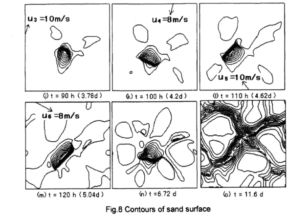
$\ln$ this simulation, the wind is assumed blow from three pairs of opposing directions. The

lntensity of the wind |s shown

on

Table 1 and the direction of the wlnd is shown

on

Fig.8 (g).

Time

duration is

10

hours.

As in the prevlous case, the initial conditions

are

calculated for the first 1000 steps (20

seconds). Thetime increment $\Delta t$ for the Navier-Stokesequation isset to$0.02\mathrm{s}$. Byusing these

lnitial conditions,

we

repeat steps $(\mathrm{i} )$-(iii)

as

mentioned in sectlon 2 and compute the change

of the shape of the sand dune. As the

same reason as

mentioned in section 3.1, n0-s|ip

condition isimposed

on

thesand surface.

Fig.8 shows the time development of sand surface contours. When winds

are

blowing form

three pairs ofopposing directions, the simulated dune, which has circular

cross

section parallel

to

x-y

plane and parabolic

cross

section parallel to both

x-z

and y-z planes, extends at four

(7)

7

Fig.8Contours of sand surface

When the sand supply is increased to two times

as

shown in Fig.9, another shape of star

dunes–complex lineardunes

are

$\mathrm{f}\mathrm{o}$rmed. ltis explained in

our

another

paper

$\mathrm{c}1\mathrm{e}\mathrm{a}\mathrm{r}1\mathrm{y}^{7)}$.

$\ovalbox{\tt\small REJECT} \mathrm{o}\mathrm{o}$

[$\mathrm{a})\mathrm{t}\underline{-}$ od

Fig. 9 Contours of sand surface ofcomplex linear dunes

4.CONCLUDING

REMARKS

$\ln$ this study, the formation of

star

dunes

are

simulated and the flow above the sand dunes

are

investigated. Onehill is placed

on

the sand sufface

as

the initialcondition.

When the winds blow from three directions, the simulated dune extends

at

three directions,

becoming the shape of

a

high central peak and three

arms

extending radially. When the winds

blow from three pairs of opposing directions, the simulated dune extends

at

four directions,

becoming theshapeof

a

high central peakandfour

arms

extending radially.

Further problem is to investigate the factors that affect the number of the

arms

ofstardunes

and the relationshipbetween thestardunes$\mathrm{w}.\mathrm{R}\mathrm{h}$ four

arms

and the complex linear dunes.

REFERENCES

1) $\mathrm{R}.\mathrm{A}$. Wasson and R. Hyde, “Factors determining desert dune typ\"e, Nature

(8)

8

$(\mathrm{f}983)$,

pp.

337-339.

2) $\mathrm{E}$ D. Mckee, 11Astudy of global sand seas, Introduction to

a

study of global sand seas”

L1S Geological Survey Professional Paper

1052

(1979), pp.1-19.

3) M. Kan and T. Kawamura, “Numerical simulation ofthe formation of the barchan sand

dun\"e,Theoretical and Applied Mechanics, $\mathrm{V}\mathrm{o}\mathrm{l}.48$(1999), pp.349-354.

4) R. Zhang, Y. Sato, M. Kan and T. Kawamura$\mathrm{f}4$

Numerical study of the effectof flow fields

on

the shape of sand dune” Theoretical and Applied Mechanic, $\mathrm{V}\mathrm{o}\mathrm{l}.52$ (2003),

pp.205-210.

5) $\mathrm{J}.\mathrm{F}$. Thompson, Z.U.A Warsi, C.W Mastin, “Numerical grid generation foundations and

applications”, Elsevier Science Pubulishing Co. Inc. (1985).

6) R. A. Bagnold, “The movementof desertsand”, Proc. Roy. Soc.A157(1963).

7) Ruyan ZHANG, Makiko KAN and Tetuya KAWAM$\mathrm{U}\mathrm{R}\mathrm{A}$, Numerical Simulation of the

Formation of the Complex Linear Dunes, Proceedings of the Sixth World Congress

on

Computational Mechanics in conjunction with the Second Asian-Pacifc Congress