Asymptotics for differentiated product demand/supply systems with many markets in the presence of national micro moments (Statistical Inference and Modelling)

全文

(1)125. Asymptotics for differentiated product. demand/supply systems with many markets in the presence of national micro moments. Yuichiro KANAZAWA[*†] International Christian University. 1. Introduction. Industrial organization literature is concerned with the structure of industries in the econ‐ omy and the behavior of firms and individuals in these industries. A dramatic shift in. the 1980s toward what Bresnahan (1989) coined the “New Empirical Industrial Organi‐ zation (NEIO),”which tries to takes advantage of the fact that individual industries are sufficiently distinct, and industry details are sufficiently important. In the NEIO, products are regarded as bundles of characteristics, and preferences are defined on those characteristics, so each consumer chooses a bundle that maximizes its utility. Consumers have different preferences for different characteristics, and hence make different choices, however. In other words, consumers are heterogeneous. Simulation is used to obtain aggregate demand from the heterogeneous consumers’ choices in the following manner: first we draw vectors of consumer characteristics from the distribution of those characteristics; second we determine the choice probability that each of the drawn consumers would make for a given value of the parameter; now we aggregate those choice probabilities into a prediction for aggregate demand conditional on the parameter vector; finally we employ a search routine that finds the value of that parameter which makes these aggregate probabilities as close as possible to the observed market shares.. The theoretical and econometric groundwork for product characteristic based de‐. mand systems dates back to the work of Lancaster (1971) [9] and McFadden (1974, 1981) [10],[11]. Applications of the Lancaster/McFadden framework, however, increased significantly after Berry, Levinsohn, and Pakes (1995, henceforth BLP(1995) [2]) showed how to circumvent a problem that had made it difficult to apply the early generation of characteristic‐based models in I.O. contexts.. [email protected] We are grateful for financial support from the Japan Society for the Promotion of Science under the. \dag er. Grant‐in‐Aid for Scientific Research (B) ı5H03333, Grant‐in‐Aid for Challenging Research (Exploratory) 17K18703 , and from the Research Institute for Mathematical Sciences, a Joint Usage/Research Center located in Kyoto University..

(2) 126 The early generation of models did not allow for unobserved product characteris‐ tics. Consumer goods typically are differentiated in many ways. As a result even if the econometricians measured all the relevant characteristics, they could not expect to obtain. precise estimates of their impacts. One solution proposed in Berry (1994) [ı] is to put in. the ‘ important’ differentiating characteristics and an unobservable, say \xi , which picks. up the aggregate effect of the multitude of characteristics that are being omitted. Often the econometricians find that there is not enough information in product level demand data to estimate the entire distribution of preferences with sufficient precision. This should not be surprising given that they are trying to estimate a whole distribution of preferences from just aggregate choice probabilities. The literature has added information in two ways: One is to add an equilibrium assumption and work out its implications for the estimation of demand parameters, the other is to add more data. It is not surprising that when the pricing system is added to the demand system, the. precision of the demand parameters estimates tends to improve (see, BLP (1995) [2]).. Almost all of it has assumed static or myopic profit maximization, and that one side of the transaction has the power to set prices while the other can only decide whether and what to buy conditional on those prices. However, models in marketing science started. looking one period ahead (see, Che, et al. (2007) [6], Kamai and Kanazawa (2016) [8]). with interactions between manufacturers and a retailer factored in.. On adding more data, there are a number of types of micro data that might be avail‐ able: Surveys that match individual characteristics to a product chosen by the individual (point‐of‐sales data); Surveys providing information on the proprietary consumer ’ s sec‐. ond choice (Berry, Levinsohn, and Pakes (2004) [3]); Alternatively, the econometricians may have access to summary statistics that provide information on the joint distribu‐. tion of consumer and product characteristics (Petrin 2002 [17]). Petrin (2002) proposes. a technique for obtaining more precise estimates of demand and supply curves when the econometricians are constrained to market‐level data. The technique allows them to augment market share data with information relating the average demographics of consumers to the observable characteristics‐Myojo and Kanazawa (2012) called “discrim‐ inating attributes”’‐of products they purchase that determines a subset of products in. the market. Petrin (2002) states that “ [t]his extra information plays the same role as consumer‐level data (p.705, [17]). Berry, Linton, and Pakes (2004) [4] provides asymptotic theory of the estimate of the demand system objective function as the number of products increases in one (national) market. The paper shows that, provided one accounts for simulation and sampling error in the estimate of the objective function, standard approximations to the limit distribu‐. tion work (see, for e.g. Pakes and Pollard, 1989 [16]). Myojo and Kanazawa (2012) [12] provides a sharper asymptotic variance‐ covariance of the estimate of the demand than. Berry, Linton, and Pakes (2004) by adding the pricing equation and micro moment ob‐ jective functions as the number of products increases in one (national) market. For durable goods like automobiles, the number of models increased from somewhere in the 150 ’s in 1980s to in the 260 ’s in 2018. Asymptotic theories of Berry, Linton, and. Pakes (2004) and Myojo and Kanazawa (2012) presuppose such a market. On the other hand, for many non‐durable consumer good products, the number of product offering is.

(3) 127 limited because of the limited shelf space at the retail outlets. In Nevo (2001), for example,. there are 1124 markets and 24 products.1) Therefore a different type of asymptotics, the one in the number of markets, is needed.. Freyberger (2015) [7] provides asymptotically normal biased parameter estimate (that depends on the number m of markets, the fixed number R of simulation draws from the distribution of consumers to calculate the observed market share of the demand system. objective function) for a fixed number of products as the number of markets increases. It also provides how the leading asymptotic bias terms can be eliminated by using an analytic bias correction method.. Asymptotic bias is generated because, for each market, its participating households are self‐selected and unique in its own way. As a result simply increasing the number of such markets will not do. One general estimation idea when you have estimates in many comparable but heterogeneous subgroups within a population is to combine the individual estimates, each unbiased, to manufacture an overall unbiased estimate, using the local variances and overall variance between subgroup means to select the best linear estimator. An approach for the current problem along this idea is to alter the number. of simulation draws from the fixed. R. in Freyberger (2015) to market‐dependent R_{m} to. reflect the population. This approach should work in theory, but a proper choice of R_{m} presupposes we know the market‐by‐market variation of the consumer preferences, the exact knowledge we are trying to estimate. In reality, different portions of the population may still be over‐ or under‐represented as we increase the number m of markets.. If we wish to have a data‐driven method as an alternative to analytic (asymptotic) bias correction proposed by Freyberger (2015), however, there is another idea we can employ (for non‐durable product markets with a limited number of product offering), however. That is, for these markets, information that encompasses many regions are available, and we can take advantage of such information to adjust the bias. In this manuscript, we show that we can pursue the second idea, namely, we can achieve the data‐driven asymptotic. bias correction by incorporating 1) the pricing (profit maximizing) equation for national suppliers and 2) the national micro moment regarding consumers as the number m of markets increases.. 2. Method. We assume the same finite set of products, j=1,. J,. is available in each regional. market.2) We also assume each consumer only participates in one market and chooses one. product including “outside”good that maximizes his/her utility within that market. The price and the unobserved product characteristic of the same product may as well vary from one market to the other because of the differences in demographics among markets. ı ) We study non‐durable goods such as ready‐to‐eat cereals because serious policy implications abound for markets of such non‐durable goods: For instance, Nevo(2001) [14] claims that “Previous researchers have concluded that the ready‐to‐eat cereal industry is a classic example of an industry with nearly. collusive pricing behavior and intense non‐price competition” (p.307).. 2)_{This} simplifying assumption can be relaxed so that the set of products available can differ somewhat by region..

(4) 128 2.1. Data. We suppose the following information is available: 1) observed exogenous product char‐ acteristics x_{j}=(x_{2j}, \ldots, x_{Kj})^{T}, (K-1)\cross 1 vector, other than price and the market‐by‐ market price p_{j}^{m} of products j, j=1 , , J;2 ) observed market‐by‐market share vector. s_{j}^{m,n_{m} ,. of products j, j=1,. of size. n_{m} ,. J,. m=. ı,. M,. in market. m. estimated from a sample. independent with respect to m;3 ) An estimate \eta_{kq}^{N} of k‐th, k=1,. K,. ob‐. served demographic characteristic of consumers who choose q‐th discriminating attribute. This estimate is constructed from a national sample of N consumers, independent of the sample of size n_{m}^{3)}. We also suppose there is a national database (e.g. the aforementioned CE‐PUMD, I with their K\cross 1 observed demographics v_{i}^{m}= for instance) of consumer i, i=1,. (\nu_{i1}^{m}, \ldots, \nu_{iK}^{m})^{T}\in\Re^{K} whose true distribution is. P^{0} . This national database, we suppose,. identifies the market each consumer participates by his/herregion/ market indicator m=1,. M . We can draw T consumers to match the. \eta_{kq}^{N}. m,. above. With this national. database with region indicator, we can construct region‐by‐region databases indexed by m. . We can randomly draw R_{m} demographics4) from this regional database to match. the s_{j}^{m,n_{m} whose observed demographics are now indexed by m so that demographics \nu_{i}^{m}=(\nu_{i1}^{m}, \ldots, \nu_{iK}^{m})^{T}\in\Re^{K} whose true distribution P^{0m}. 2.2. K\cross 1. observed. Demand side. Reflecting the heterogeneity of consumers, we define the model calculated probability \sigma_{ij}^{m} of consumer i choosing product j in market m to be obtained from the random coefficient utility of consumer i with observed demographics \nu_{i}^{m} in market m for product j as. U_{ij}^{m} = x_{j}^{mT} \cdot\beta+\sum_{k=1}^{K}\pi_{k}x_{jk}\nu_{ik}^{m}+\xi_ {j}^{m}+\epsilon_{ij}^{m}. ,. (1). with the observed K\cross 1 product characteristics vector x_{j}^{m}=(p_{j}^{m}, x_{j}^{T})^{T} that may in‐ clude a constant or product dummies, the demand‐side K\cross 1 parameter vector \beta= (\beta_{1}, \ldots, \beta_{K}) associated with the observed product characteristics, K\cross 1 parameter vec‐ tor \Pi=(\pi_{1}, \ldots, \pi_{K}) associated with the observed demographics, unobservable \xi_{j}^{m} likely to be correlated with price p_{j}^{m} , and with unobservable idiosyncratic taste \epsilon_{ij}^{m} assumed to be i.i. d . type‐I extreme value.. The conditional probability \sigma_{ij}^{m} of choosing product j in market. \sigma_{ij}^{m}=\frac{\exp(x_{j}^{mT}\cdot\beta+.\sum_{k=1}^{K}\pi_{k}x_{jk} \nu_{ik}+\xi_{j}^{m}){1+\sum_{j=1}\exp(x_{j}^{mT}\beta+\sum_{k=1}^{K}\pi_{k} x_{jk}\nu_{ik}+\xi_{j}^{m}). m. obtained from (1) (2). 3)We do not believe that the independent‐source requirement is so restrictive or unrealistic. We could. sample individuals from the Consumer Expenditure Survey Public‐Use Microdata (CE‐PUMD) to sim‐ ulate market shares of products, whereas the additional micro moment could be obtained from publicly available sources independent of the CE‐PUMD because what we require is the aggregate estimates and not the sample itself—most ıikely to be proprietary—from which these aggregate estimates are computed. 4) These two draws T and are R_{m} are assumed independent..

(5) 129 is a map from consumer i ’s tastes v_{i}^{m} , a demand‐side parameter 2K\cross 1 vector \theta_{d}= (\beta^{T}, \Pi^{T})^{T}\in\Re^{2K} , and the set of characteristics of all products p^{m}=(p_{1}^{m}, \ldots,p_{J}^{m})^{T}, a J\cross 1 vector, X=(x_{1}, \ldots, x_{J}), a(K-1)\cross J matrix, \xi^{m}=(\xi_{{\imath}}^{m}, \ldots, \xi_{J}^{m})^{T}, a J\cross 1 vector,. and is thus denoted as. \sigma_{ij}^{m}(p^{m}, X, \xi^{m}, v_{i}^{m}, \theta_{d}) .. The BLP framework generates the vector of the model‐calculated J\cross 1 market share vector \sigma^{m}=(\sigma_{1}^{m}, \ldots, \sigma_{J}^{m})^{T} in market m by aggregating over the individual choice prob‐ ability in (2) with the true distribution P^{0m} of the consumer tastes \nu_{i}^{m} as. \sigma_{j}^{m}(p^{m},X,\xi^{m},\theta_{d},P^{0m})=\int\frac{\exp(x_{j} ^{mT}\cdot\sqrt{}+.\Sigma_{k=1}^{K}\pi_{k}x_{jk}\nu_{ik}+\xi_{j}^{m}){1+\Sigma_ {j=1}\exp(x_{j}^{mT}\sqrt{}+\Sigma_{k=1}^{K}\pi_{k}x_{jk}\nu_{ik}+\xi_{j}^{m}) dP^{0m}. .. (3). We assume the set of exogenous product characteristics x_{j}= (x_{2j} , x_{Kj})^{T}, j= , J , is a random sample from the underlying population of product characteristics. J are a random sample of unobserved We also assume that, given x_{j}' s, \xi_{j}^{m}, j=1, characteristics from the portion of the population representing market m . Thus, x_{j} are assumed independent across j , and \xi_{j}^{m} are independent conditionally on x_{j} , while p^{m}=(p_{1}^{m}, \ldots,p_{J}^{m})^{T} are not, in general, independent across j since they are endogenously determined in market m as functions of others’ and its own product characteristics. 1,. Note that these market shares are still random variables due to the stochastic nature. of the product characteristics. X. and \xi^{m} . If we evaluate. \sigma_{j}^{m}(p^{m}, X, \xi^{m}, \theta_{d}, P^{0m}). at. \theta_{d}^{0},. where \theta_{d}^{0} is the true parameter value, we have the “conditionally true”market shares s_{j}^{m0} given the product characteristics (p^{m}, X, \xi^{m}) in the portion of the population representing market. m. , i.e.,. \sigma^{m}(p^{m}, X, \xi^{m}, \theta_{d}^{0}, P^{0m})\equiv s^{0^{m}}. (4). BLP (1995) [2] provides general conditions under which there is a unique solution for the \xi^{m} for the equation. \sigma^{m}(p^{m}, X, \xi^{m}, \theta_{d}, P^{m})=s^{m}. (5). for every (p^{m}, X, \theta_{d}, P^{m}) . If we solve (5), at any (\theta_{d}, s^{m}, P^{m})\neq(\theta_{d}^{0}, s^{0^{m}}, P^{m0}) , the in‐ dependence assumption for the resulting \xi_{j}(X, \theta_{d}, s^{m}, P^{m}) no longer holds. On the other hand, if we solve the identity in (4) with respect to \xi^{m} under the conditions to guarantee the uniqueness of the \xi^{m} in (5), we are able to retrieve the original \xi_{j}^{m}(X, \theta_{d}^{0}, s^{0}, P^{m0}) , which we assume are conditionally independent across j given x=(x_{2j}, \ldots, x_{Kj})^{T}. Since the econometrician do not have access to P^{m0} nor s^{0^{m}}, he/she must use the R_{m} random draws from P^{m0} and the observed share. s^{m,n_{m}}=(s_{1}^{m,n_{m}}, \ldots, s_{J}^{m,n_{m}}). which is. usually estimated from a random sample of size n_{m} . The R_{m} random draws are assumed independent of the sample of size n_{m} above. The observed market share s_{j}^{m,n_{m} of product j in market. i. m. is thus matched with the model‐calculated market share. choosing product j in market. m. from m‐th reginal database as. s_{j}^{m,n_{m} = \frac{1}{R_{m} \sum_{i=1}^{R_{m} \sigma_{ij}^{m}(p^{m}, X,\xi^ {m}, \theta_{d}, P^{R_{m},m}). ,. \sigma_{j}^{m}. of consumer. (6).

(6) 130 where P^{R_{m},m} is the empirical measure that signifies a random sample of R_{m} is taken from the database indexed by the market index m . We denote the \xi as a solution to the J si‐ J as \xi(\theta_{d},p^{m}, X, s^{m,n_{m}}, P^{R_{m},m}) . multaneous equations (4) with J unknown \xi_{j}, j=1, m as We assume the mean independent conditions to hold for each market m=1,. E(\xi_{j}^{m}|X)=0 ,. (7). with probability 1 and to have a finite conditional variance. \sup_{1\leq m\leq M}\max_{1\leq j\leq J}E( \xi_{j}^{m})^{2}|x_{j})<\infty, with probability 1. We assume there is a. J\cross. Mı matrix demand‐side instruments. Z_{d}=(z_{1}^{d}, \ldots, z_{J}^{d})^{T}. whose j‐th component z_{j}^{d} can be written further as z_{j}^{d}(x_{1}, \ldots, x_{J})\in\Re^{M_{1}} , where \Re^{(K-1)\cross J}arrow\Re^{M_{1}} , for j=1, J such that its the resulting M_{1}\cross 1 vector. E(Z_{d}^{T}\xi^{m}(\theta_{d}^{0},p^{m}, X, s^{0^{m}}, P^{m0}))=0 , in view of (7), where. 0. z_{j}^{d}(\cdot). :. (8). is a M_{1}\cross 1 vector of zeroes, if we assume, for moment, that we. know the underlying taste distribution of P^{m0} and we are able to observe the true market share s^{0^{m}} The expectation in (8) is taken with respect \xi conditionally on X , and then with respect to. X.. It should be noted that the demand side instruments z_{j}^{d} for product j are assumed to be a function of the exogenous characteristics not only of its own, but of the other products in the market. This is because the instruments by definition must correlate with the product characteristics p_{j}^{m} , and these endogenous price are determined by both its own and its competitors’ product characteristics.. Then the sample counterpart of this condition employing the solution to (6) is the. following M_{1}\cross 1 vector. G_{M}^{d}( \theta_{d}, \{s^{m}\}, \{P^{R_{m} \})=\frac{1}{M}\sum_{m=1}^{M}Z_{d} ^{T}\xi_{j}^{m}(\theta_{d},p^{m}, X, s^{m,n_{m} , P^{R_{m},m}) 2.3. .. (9). Supply side. The supply side model formulates the pricing equations for the J products marketed. We assume an oıigopolistic market where a finite number of suppliers provide multiple products to all M markets. Suppliers (m=1, \ldots, F) producing \mathcal{J}_{f} are maximizers of profit from the combination of products they offer. A profit function of supplier f in market m is given for by. PR_{f}^{m}= \sum_{j=1}^{J}(p_{j}^{m}-mc_{j}^{m})\sigma_{j}^{m}(p^{m}, X, \xi^{m}, \theta_{d}, P^{m})\cdot I^{m}. (10). where j\in \mathcal{J}_{f} and mc_{j}^{m} is the marginal cost of product j in market m and I_{m} is the size of population in market m . Then, the total profit of the firm f is \Sigma_{m=1}^{M}PR_{f}^{m}..

(7) 131 131 Since consumer only participates in his/her home market, maximizing the profit func‐ tion in each regional market m separateıy leads to maximizing the total profit for each firm.. Assuming BertrandNash pricing provides the first‐order condition for the product j of the manufacturer. m. as. \sigma_{j}^{m}(p^{m}, X, \xi^{m}, \theta_{d}, P^{m})+\sum_{h\in \mathcal{J} _{f} (p_{h}^{m}-mc_{h}^{m})\frac{\delta\sigma_{h}^{m}(p^{m},X,\xi^{m},\theta_{d} ,P^{m}) {\delta p_{j}^{m}. ,. (11). This equation can be expressed in matrix form as. \sigma^{m}(p^{m}, X,\xi^{m}, \theta_{d}, P^{m})+\triangle^{m}(p^{m}-mc^{m})=0 , where. \Delta^{m}. is the. J\cross J. (12). non‐singuıar matrix whose (j, h) element is defined as. \triangle_{jh}^{m}=\{\begin{ar ay}{l } \delta\sigma_{h}^{m}(p^{m}, X, \xi^{m}, \theta_{d}, P^{m})/\delta p_{j}^{m} if the products j and h are produced by the same firm; 0, otherwise \end{ar ay} We solve (12) with respect to. mc^{m}. as. mc^{m}=p^{m}+(\Delta^{m})^{-1}\sigma^{m}(p^{m}, X, \xi^{m}, \theta_{d}, P^{m}) .. (13). Suppose that the observed cost shifters w_{j} consist of exogenous w_{1j}\in\Re^{L_{1}} as well as endogenous w_{2j}\in\Re^{L_{2}} , and thus we write w_{j}=(w_{1j}^{T}, W_{2j}^{T})^{T}, a(L_{1}+L_{2})\cross 1 vector, and W=(w_{1}, \ldots, W_{J})^{T}, a J\cross(L_{1}+L_{2}) matrix. The exogenous cost shifters include not. only the cost variables determined outside the market under consideration (e.g., factor price), but also the product design characteristics suppliers cannot immediately change in response to fluctuation in demand.. The cost variables determined by the market equilibrium (e.g., production scale) are. treated as endogenous cost shifters. As in the formulation of x_{j} on the demand side, we J , is a random sample from assume that the set of exogenous cost shifters w_{1j}, j=1, the underlying population of cost shifters. We also assume as in the formulation of \xi_{j}^{m},. given w_{1j}' s, \omega_{j}^{m}, j=1,. J,. is a random sample of the unobserved cost shifter from. the portion of the population representing market m . Thus, w_{j} are assumed independent across j , and \omega_{j}^{m} are ind ependent conditionally on w_{j} , although w_{2j} are, in general, not independent across j as they are determined in the market as functions of cost shifters of other products.. We define the marginal cost mc_{j}^{m} as an implicit function of the observed cost shifters. w_{j} and the unobserved cost shifter. \omega_{j}^{m}. in market. m. as. g(mc_{j}^{m})=w_{j}^{T}\theta_{c}+\omega_{j}^{m} ,. (14). where g() is a monotonic function and \theta_{c}\in\Theta_{c} is a vector of cost parameters. Although the choice of g(\cdot) depends on the application, we assume that g(\cdot) is continuously differentiable with a finite derivative for all realizable values of cost. Define. g(x)\equiv(g(x_{1}), \ldots, g(x_{J}))^{T}.. Then the J\cross 1 cost‐side unobserved cost shifter vector obtains as. \omega^{m}(p^{m}, X, \xi^{m}, \theta_{d}, P^{m})=g(p^{m}+(\Delta^{m})^{-1} \sigma^{m}(p^{m}, X,\xi^{m}, \theta_{d}, P^{m}))-W\theta_{c} .. (15).

(8) 132 Similar to the demand‐side unobservables, the unobserved cost shifter \omega_{j}^{m} is assumed to be mean independent of the exogenous cost shifters W_{1}=(w_{11}, \ldots, w_{1J}) , and satisfy. E(\omega_{j}^{m}|W_{1})=0 ,. (16). with probability 1 and to have a finite conditional variance. \sup_{1\leq m\leq M}\max_{1\leq j\leq J}E( \omega_{j}^{m})^{2}|w_{1j})<\infty, with probability 1. Similar to the demand side, we assume there is a J\cross M_{2} matrix supply‐side instruments Z_{c}=(z_{1}^{c}, \ldots, z_{J}^{c})^{T} whose j‐th component z_{j}^{c} can be written further as z_{j}^{c}(w_{11}, \ldots, w_{1J})\in \Re^{M_{2}} , where z_{j}^{c}(\cdot) : \Re^{(L_{1})\cross J}arrow\Re^{M_{2}} , for j=1, J such that its the resulting M_{2}\cross 1. vector. E(Z_{c}^{T}\omega^{m}(\theta_{d}^{0},p^{m}, X, s^{0^{m}}, P^{m0}))=0 , in view of (16), where. 0. (17). is a M_{2}\cross 1 vector of zeroes, if we assume, for moment, that we. know the underlying taste distribution of P^{m0} and we are able to observe the true market. share s^{0^{m}} The expectation in (17) is taken with respect. \omega. conditionally on. W,. and then. with respect to W. We also note that some of the exogenous product characteristics x_{j} affect the price. of the product because they affect manufacturing cost. Thus, those x_{j} may be included among the exogenous cost shifters w_{1j} if they are uncorrelated with the unobservable cost shifter. \omega_{j}^{m}. for j=1,. J.. Then the sample counterpart of this condition is the following M_{2}\cross 1 vector. G_{M}^{c} ( \theta, \{s^{m}\}, \{P^{R_{m} \})=\frac{1}{M}\sum_{m=1}^{M}Z_{c} ^{T}\omega_{j}^{m}(\theta,p^{m}, X, s^{m,n_{m} , P^{R_{m},m}) where. \theta=(\theta_{d}, \theta_{c}) .. 2.4. Micro moments. ,. (18). Market summaries such as the average demographics of consumers who purchased a spe‐ cific type of product are publicly available, even if detailed individual‐level data such as purchasing histories are not. A discriminating attribute is an observable product charac‐ teristic of products that determines a subset of products in the market, those products that possess the attribute. We denote the set of products with discriminating attribute q as Q_{q} , and the consumer’s choice as C_{i} . We will write the event “consumer i chooses discriminating attribute q ” as C_{i}\in Q_{q} . A consumer may choose multiple discriminat‐ ing attributes. We assume that there is a finite number of discriminating attributes q=1, N_{p} , and the market share of each discriminating attribute is positive, i.e., Pr\{C_{i}\in Q_{q}|X, \xi(\theta_{d}^{0},p^{m}, X, s^{0^{m}}, P^{m0})\}>0 for all q in 1, N_{p}..

(9) 133 We assume that the joint density of demographics \nu_{i}^{m} is of bounded support, m= M . In market m , consumer i's k‐th observed demographic \nu_{ik}^{m}, k=1 , , K is averaged over all consumers choosing discriminating attribute q in the population to obtain the conditional expectation An example of this conditional expectation would be the expected value of family size of consumers in the subpopulation P^{m0} corresponding to the market m who purchased a box of ready‐to‐eat cereal with high sugar content. We assume that \eta_{kq}^{0^{m} has a finite mean 1,. \eta_{kq}^{0^{m}}=E\{\nu_{ik}^{m}|C_{i}\in Q_{q}, X, \xi(\theta_{d}^{0},p^{m}, X, s^{0^{m}}, P^{m0})\}.. i.e., E_{X,\xi}\{\eta_{kq}^{0^{m} \}<\infty and V_{X,\xi}\{\eta_{kq}^{0^{m} \}<\infty for k=1, K, q= M. N_{p} , m ı, It may be possible to match the the sample counterpart of \eta_{kq}^{0^{m} market‐by‐market with. and variance for all 1,. J,. =. the sample counterpart of. E\{\nu_{ik}^{m}|C_{i}\in Q_{q}, X, \xi(\theta_{d}^{0}, p^{m}, X, s^{0^{m}}, P^{m0})\}. whenever a finer. data set of consumers’ market‐by‐market average choice of discriminating attribute q is available. If so, finite sample performance of the estimated parameter would be better. If such a data set is not readily available as we assume here, however, we proceed as fol‐ lows: Notice, as marrow\infty , we have the sample counterpart of \sum_{m={\imath} ^{M}\eta_{kq}^{0^{m} /M to converge in probability to \eta_{kq}^{0} for any k and g by virtue of the weak law of large numbers. Similarly the. \Sigma_{m=1}^{M}E\{\nu_{ik}^{m}|C_{i}\in Q_{q}, X, \xi(\theta_{d}^{0}, p^{m}, X, s^{0^{m} , P^{m0})\}/M to converge E\{\nu_{ik}|C_{i}\in Q_{q}, X, \xi(\theta_{d}^{0},p, X, s^{0}, P^{0})\} where p=(p^{1}, \ldots,p^{m}) .. sample counterpart of in probability to. Let Pr\{d\nu_{ik}|C_{i}\in Q_{q}, X, \xi(\theta_{d}, p, X, s^{0}, P^{0})\} be the conditional density of consumer i^{1}s demographics y_{ik} given his/her choice of discriminating attribute q and product charac‐ teristics (p, X, \xi (\theta_{d},p, X, s^{0}, P0)) . Since the conditional expectation \eta_{dq}^{0} can be written as. E\{\nu_{id}|C_{i}\in Q_{q}, X, \xi(\theta_{d},p, X, s^{0}, P^{0})\}. = \int\nu_{id}Pr\{dv_{id}|C_{i}\in Q_{q}, X, \xi(\theta_{d},p, X, s^{0}, P^{0} )\}. = \frac{f\nu_{id}Pr\{C_{i}\in Q_{q}|X,\xi(\theta_{d},p,X,s^{0},P^{0}),\nu_{id} \}P^{0}(d\nu_{id}) {P_{\Gamma}\{C_{i}\in Q_{q}|X,\xi(\theta_{d},p,X,s^{0},P^{0}) \} = \frac{\int\nu_{id}Pr\{C_{i}\in Q_{q}|X,\xi(\theta_{d},p,X,s^{0},P^{0}), \nu_{i}\}P^{0}(d\nu_{i}) {Pr\{C_{i}\in \mathcal{Q}_{q}|X,\xi(\theta_{d},p,X, s^{0},P^{0})\} \int\nu_{id}\frac{\Sigma_{j\in Q_{q} \sigma_{ij}(X,\xi(e_{d}, {\bul et_{j\in \mathcal{Q}_{q} \sigma_{j}(X,\xi(\theta_{d}p,X,s^{0 }\bul et),\theta_{d},P^{0}) P^{0}(dv_{i}) =. ,. we can form an identity, which is the basis for additional moment conditions. \eta_{dq}^{0}-\int\nu_{id}\frac{\Sigma_{j\in\mathcal{Q}_{q}\sigma_{ij}(X,\xi (\theta_{d}^{0},pX,s^{0},P^{0}),\nu_{i};\theta_{d}^{0}){\Sigma_{j\in \mathcal{Q}_{q}\sigma_{j}(X,\xi(\theta_{d}^{0},pX,s^{0},P^{0}),\theta_{d}^{0}, P^{0})P^{0}(d\nu_{i})\equiv0. (19). for q=1, , K. N_{p}, k=1 , P^{0} Although is so far assumed known, we typically are not able to calculate the. second term on the left hand side of (20) analytically and will have to approximate it by T from the underlying using the empirical distribution P^{T} of i.i. d . sample v_{t}, t=1, P^{0} distribution . The corresponding sample moments G_{J,T}^{a}(\theta_{d}, p, X, s^{n}, P^{R}, \eta^{N}) , where a.

(10) 134 on the shoulder stands for additional, are. G_{J,T}^{a}( \theta_{d},p, X, s^{n}, P^{R}, \eta^{N})=\eta^{N}-\frac{1}{T}\sum_ {t=1}^{T}\nu_{t}\otimes\psi_{t}(\xi(\theta_{d},p, X, s^{n}, P^{R}), \theta_{d}, P^{R}). (20). where. \eta^{N}=(\eta_{1 }^{N},\ldots,\eta_{1N_{p}^{N},\ldots,\eta_{K1}^{N}, \ldots,\eta_{KN_{p}^{N})^{T},\psi_{t}(\xi(\thea_{d},p X,s^{n},P^{R}), \thea_{d},P^{R})= (\begin{ary}l \fcsum_{JinQl}\sgma_{t(X,xinu;}\heta_{d)sumJ\inQ_{1} sgmaJ(X,\xithe_{d}P^R) \frac{sum_JinQN{p}\sgma_t(X,xi\nu{}thea_d)\sum{Jin Q_Np}\sgma{J(X,xithe_d}P^{R) \enary}. The symbol \otimes denotes the Kronecker product. The quantity \psi_{t}(\xi, \theta_{d}, P) is the consumer t ’s model‐calculated purchasing probability of products with discriminating attribute q relative to the model‐calculated market share of the same products. Note that these additional moments are again conditional on product characteristics (p, X, \xi(\theta_{d}, s^{n}, P^{R})) ,. and thus depend on the indices J and. T.. As a result, the actual sample‐based objective function we minimize in the GMM. estimation is the sum of norm of G_{M}^{d} (\theta_{d} , {sm}, \{P^{R_{m}}\}) in (9), (18), and G_{J,T}^{a}(\theta_{d}, s^{n}, P^{R}, \eta^{N}) in (20), that is, the norm of. G_{M}^{c}(\theta , {sm}, \{P^{R_{m}}\}) in. G_{J,T}(\thea,s^{n},P^{R},\eta^{N})=(G_{MT}^{a}(\thea_{d},pX,s^{n},P\eta^ {N})G_{M}^{c\}_{\thea,\{s^m}\, {P^R_{m}\}^{\thea_{d},\{s^m}\, {P^R_{m} }J,)G_{M}^{d},). ,. (22). M_{1}+M_{2}+KN_{p}\cross 1 vector. Notice that the first two moments G_{M}^{d} and G_{M}^{c} in (22) are the sample moments M , although the third moment averaged over products m=1, G_{M,T}^{a} is averaged over a. consumers. 3. t=1,. T.. Theoretical Results. Note that in the expression G_{M,T}^{a}(\theta_{d},p, X, s^{n}, P^{R}, \eta^{N}) , there exist five distinct random‐ nesses: one from the draws of the product characteristics (X, \xi_{j}, w_{1j}, \omega_{j}) , two from the. sampling processes of consumers for s^{n} and \eta^{N} (not controlled by the econometrician), and two from the empirical distributions \{P^{R_{m} \} and P^{T} (employed by the econometri‐ cian). The impact of these randomnesses on the estimate of \theta are decided by the relative sizes of the samples—J, \{n_{m}\}, N, \{R_{m}\} , and T . Carefully operationalizing the sampling and the simulation errors obtain the following result.. Theorem 1 (Consistency and Asymptotic Normality of \theta=(\theta_{d}, \theta_{c}) ) The estima‐ tor \theta that minimizes the objective function G_{J,T}(\theta, s^{n}, P^{R}, \eta^{N})^{T}W_{m}G_{J,T}(\theta_{\mathcal{S}^{n} }, P^{R}, \eta^{N}) is consistent, and asymptotically normal at the rate of \sqrt{M} where W_{m} is a weighting matrix converging in probability to a positive definite matrix W.. Due to the limitation of the space, we omit the proof.. (21).

(11) 135 4. Simulation Results. Throughout below,. 4.1. Demand side setting. The model calculated share \sigma_{ij}^{m} is from random coefficient utility of consumer graphics \nu_{i}^{m} in market m for product j as. U_{ij}^{m}=-\alpha p_{j}^{m}+\beta_{0}x_{j}+\beta_{1}x_{j}\nu_{i}^{m}+\xi_{j} ^{m}+\epsilon_{ij}^{m} ,. i. of demo‐. (23). with the observed product characteristics x_{j}=(p_{j}^{m}, x_{j}) , the demand‐side parameters \theta_{d}= (\alpha, \beta_{0}, \beta_{1}) , unobservable \xi_{j}^{m} correlated with price p_{j}^{m} and with unobservable idiosyncratic taste. \epsilon_{ij}^{m}. assumed to be i.i. d . extreme value.. We assume there are J=20 products available to consumers of any of m markets. The observed product characteristics x_{j} and unobserved product characteristics \xi_{j}^{m} are random draws from N(3,1) and N(0,1) respectively. The consumer demographics \nu_{i}^{m} is random draws from N(0,1) and consumerls idiosyncratic term \epsilon_{ij}^{m} is assumed to be i.i. d . with type I extreme value to derive random‐coefficient logit model. The price p_{j}^{m} of product j is endogenously determined in each regional market equilibrium and differs from market to market. We set the true demand side parameters as \alpha=1.0, \beta_{0}=1.0 and \beta_{1}=0.5 . These parameter values are common to all the regional markets. We set the total number of consumers in the national market as I=10,000 and assume there exist. the same number I/M of consumers in each regional market. We draw R_{m} consumers J . We use the from these regional database to calculate \xi_{j}^{m} using (9) for j=1, “conditionally true”market‐by‐market share s^{0^{m}} using the population I=10,000 instead of the observed share s^{n_{m}} to focus on the effect of supply side and micro moments.. 4.2. Supply side setting. We assume there are F=5 oligopolistic suppliers in a national market, each producing the same numberJ_{f}=4 of products. As stated above, the same set of products are sold in all regional markets. These suppliers are assumed to have the same cost function of product j in market. m. as. mc_{j}^{m}=x_{j}\gamma+\omega_{j}^{m} , where the unobserved cost shifters. side parameter as \gamma=1.5.. \omega_{j}^{m}. are random draws from. (24) N(0,1) .. We set the cost. The true market share s^{0^{m}} and the corresponding price p^{m} are determined at the. equilibrium, and thus the values of p^{m} are obtained by solving (13), that is, a system of J‐dimensional nonlinear simultaneous equations, which is solved by an iterative Newton‐ Raphson algorithm..

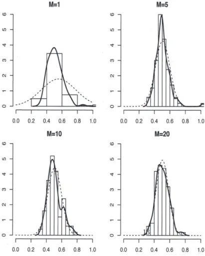
(12) 136 \overline{\overline{\#ofiternations\beta_{1}}}. \frac{R_{m}=100(fixed)withoutm\dot{ \imath} cromomentswithmicromoments(T=1, 000)}{MeanM=10.566090.565112} M=5. 0.492358. 0.496941. M=10. 0.524297. 0.506038. M=20. 0.514595. 0.494323. \frac{M=400.5151110.498628}{S.E.M=10.5798770.239662} M=5. 0.237166. 0.0702588. M=10. 0.172493. 0.0696279. M=20. 0.109436. 0.0609522. M=40. 0.070198. 0.0591414. Table ı: Mean and standard error of \beta_{1} with micro moments. 4.3. Instruments. We construct three instruments from X for the product j produced by f:x_{j} itself, the sum of x_{k} within the firm f except x_{j} , and the sum of x_{k} over the.firms other than f , as. BLP (1995) proposed. We use these three instruments for demand‐ as well as supply‐side.. 4.4. Micro moment setting. We assume that information is available on (a) the expected value of \nu_{i}^{m} over con‐ sumers who choose products priced higher than the average national price and (b) the expected value of v_{i}^{m} over consumers who choose products with x_{j} greater than the av‐ erage of x_{j} . We draw T consumers independent of R_{m} from the national population database to construct sample analogue of moment in (20). Since we use two discrimi‐ nating attribute—(a) and (b) above, we have N_{p}=2 . Similarly we compare two-p_{j}. and x_{J}—product characteristics, so we have K=2 . Also there are two instruments on demand‐ as well as supply‐side, M_{1}=M_{2}=2 . Therefore G_{J,T}(\theta, s^{n}, P^{R}, \eta^{N}) is M_{1}+M_{2}+KN_{p}\cross 1=(2+2+2\cross 2)\cross 1=8\cross 1 vector. Since the objective function we use is G_{J,T}(\theta, s^{n}, P^{R}, \eta^{N})^{T}W_{m}G_{J,T}(\theta, s^{n}, P^{R}, \eta^{N}) , we need 8\cross 8 weight matrix W. For W , we used 8\cross 8 identity matrix. Notice that the calculation may not be as efficient relative to when we use the optimal weighting matrix. We set the true parameter values to be our initial values.. We are most interested in the the consum.er heterogeneity (random coefficient) param‐ eter \beta_{1} . For the parameter \beta_{1} , see Table 1 and Figure 1. We observe the following: (1) The finite sample estimates with micro moments seems asymptotically unbiased, while the estimates without remain biased; (2) The finite sample estimates with micro moments seems more accurate than the estimates without; (3) As expected, the effect of the micro moments wanes as the number m of markets grows. Due to the limitation of the space, we omit the results for the other parameter estimates..

(13) 137. Figure 1: Histogram of \beta_{1} with the micro moments. Solid lines are density estimates and dashed lines are normal curve with the estimated mean and standard error.. M=1. M=5. (o. (D. [\Omega. [f). \triangleleft. \triangleleft. co. co. c. ou. 0. 0. 0.0. 0.2. 0.4. 0.6. 0.8. 1.0. 0.0. M=10 (D. \iota t). 0. \triangleleft. v. co. co. ou. ou. 0. 0. 0.2. 0.4. 0.6. 0.8. 1.0. 0.4. 0.6. 0.8. 1.0. 0.8. 10. M=20. (D. 0.0. 0.2. 0.0. 0.2. 0.4. 0.6.

(14) 138 5. Conclusion and Discussion. Overall, we found the following: Improvement in bias correction as expected, but slight standard error improvement is surprising; National micro moments greatly helps us to evaluate the heterogeneity of consumers when the number of market is small ( i.e. the information is limited) both in terms of standard error and bias; Contribution from adding micro moment decreases as the number of markets increases as expected. One note of caution for practitioners: With a small sample size T of demographics to construct micro moments, the accuracy of estimates seems to suffer.. References [1] Berry, S. (1994), “Estimating Discrete Choice Models of Product Differentia‐ tion,”RAND Journal of Economics, Vol 25(2), 242‐262.. [2] Berry, S., J. Levinsohn and A. Pakes (1995), “Automobile Prices in Market Equilib‐ rium,”Econometrica, Vol.63, 841‐890.. [3] Berry, S., J. Levinsohn and A. Pakes (2004), “Estimating Differentiated Product. Demand Systems from a Combination of Micro and Macro Data: The New Car. Model,”Journal of Political Economy, vol. 112(1), 68‐105.. [4] Berry, S., O. Linton and A. Pakes (2004), “Limit Theorems for Estimating the Pa‐ rameters of Differentiated Product Demand Systems,”Review of Economic Studies,. Vol.71613‐654.. [5] Bresnahan, T. F. (1989), (Empirical Studies of Industries with Market Power.”In Handbook of Industrial Organization, vol. 2, ed. Richard Schmalensee and Robert D. Willig, 101157. Amsterdam: North Holland.. [6] Che, H., Sudhir, K. and Seetharaman, P.B. (2007), “Bounded Rationality in Pric‐ ing under State‐Dependent Demand:. Do Firms Look Ahead, and If So, How Far?” Journal of Marketing Research, Vol. 44 (3), 434‐449.. [7] Freyberger, J. (2015), “Asymptotic theory for differentiated products demand models with many markets.”Journal of Econometrics, vol. 185, 162‐181.. [8] Kamai, T. and Kanazawa (2016), “Is product with a special feature still rewarding? The case of the Japanese yogurt market Cogent Economics & Finance, Vol. 4(1).. [9] Lancaster, K. (1971), Consumer Demand: A New Approach, Columbia University Press, New York.. [10] McFadden, D. (1974), “Conditional Logit Analysis of Qualitative Choice Behavior,”in P. Zarembka eds. Frontiers of Econometrics, Academic Press, New York.. [11] McFadden, D. (1981), “Econometric Models of Probabilistic Choice,”in C. Manski and D. McFadden, eds. Structural Analysis of Discrete Data with Econometric Ap‐ plications, MIT Press, Cambridge, MA..

(15) 139 [12] Myojo, S., Kanazawa, Y. (2012), “On Asymptotic Properties of the Parameters of Differentiated Product Demand and Supply Systems When Demographically‐ Categorized Purchasing Pattern Data are Available International Economic Review, Vol.53(3), 887‐938.. [13] Nakayama, K. (2014), “Simulation Studies for Asymptotic Properties of the Param‐ eters of Differentiated Product Demand and Supply Systems When the Number of Markets Increases University of Tsukuba, Master Thesis.. [14] Nevo, A. (2001) “Measuring Market Power in the Ready‐to‐Eat Cereal Indus‐ try,”Econometrica, vol. 69 (2), 307‐342.. [15] Nelder, J., and R. Mead (1965), “A simplex method for function minimiza‐ tion,”Computer Journal 7, 308‐313.. [16] Pakes, A. and D. Pollard (1989), “Simulation and the Asymptotics of optimization Estimators,”Econometrica, vol. 57(5), 1027‐1057. [17] Petrin, A. (2002) “Quantifying the Benets of New Products: The Case of the Mini‐ van,”Journal of Political Economy, Vol.110, 705‐729.. [18] Suga, M. (2013), “On Asymptotic Properties of an Estimator for Demand When the Number of Markets Increases,”University of Tsukuba, Master Thesis.. [19] Takeshita, K. (2015), “CAN properties of the random‐coefficient model of demand for nondurable consumer goods in the presence of national micro moments: A simulation study,”University of Tsukuba, Master Thesis..

(16)