A
computer
assisted proof of the
Kolmogorov problem
of
incompressible
viscous
fluid
Yoshitaka Watanabe Kyushu University
Abstract
A computer-assisted proofwhich proves the existence of non-trivial steady-state solu-tions forthe Kolmogorov flowsispresented. The method is basedontheinfinite-dimensional
fixed-point theoremusingNewton-likeoperator. This paper also proposes a numerical
ver-ification algorithm which generates automaticallyon a computer aset including the exact
non-trivial solution with mathematicalrigorous error bounds. All discussed numerical
re-sultsaretakeninto accountofthe effects ofroundingerrorsin thefloating point
computa-tions.
1
Introduction
Consider the Navier-Stokes equations:
$u_{t}+uu_{x}+vu_{y}= \nu\Delta u-\frac{1}{\rho}p_{x}+\gamma\sin(\frac{\pi y}{b})$ , (1)
$v_{t}+uv_{x}+vv_{y}= \nu\triangle v-\frac{1}{\rho}p_{y}$, (2)
$u_{x}+v_{y}=0$, (3)
where $(u, v)$, $\rho,$ $p$ and $\nu$ are velocity vector,
mass
density, pressure and kinematic viscosity,respectively and $\gamma$ is a constant representing the strength of the sinusoidal outer force. Also $*\xi$ $:=\partial/\partial\xi(\xi=t, x, y)$ and
$\triangle$ $:=\partial^{2}/\partial x^{2}+\partial^{2}/\partial y^{2}$
.
The flowregion isarectangle $[-a, a]\cross[-b, b]$and the periodic boundary conditions are
imposed
in both directions. The aspect ratio isdenoted by $\alpha$ $:=b/a.$
The above equations (1-3) describe the Navier-Stokes flows in a two-dimensional flat torus
under a special driving force proposed by Kolmogorov [1, 5], [6, Chapter 5] and have a basic solution which is written as
$(u, v,p)=(k\sin(\pi y/b), 0, d)$,
where $k$ $:=b^{2}\gamma/(\pi^{2}v)$ and $d$ is any constant. It is known that non-trivial solutions bifurcate
from the basic solution at a certain Reynolds number, which is defined below, if and only if
$0<\alpha<1[1]$. Okamoto-Shoji[5] computed numericallybifurcation diagramswith the Reynolds
number as a bifurcation parameter varying theaspect ratio asasplittingparameter. They also
strongly suggested stability of the bifurcating solutions for all $0<\alpha<1$. Nagatou [2] took
an another approach to this stability problem byemploying the theoryof verified computation
and showed that the stability ofthe bifurcating solutions is mathematical rigorously assured
for the cases of$\alpha=0.4$, 0.7 and 0.8.
In the previouspaper [10], weproposeda method toprove the existenceandthelocalunique
number and aspect ratio by a computer-assisted proofwith some verified results. It was also the first theoretical results to the non-trivial solutions of the equations (1–3).
The aim of this paper is to apply
our
other verification method: FN-Int[3, 4, 9] to prove the existence of the steady-state solutions ofproblem (1-3) andto ascertain its effectiveness inthe actual numerical computation.
In FN-Int, the equation is decomposed into the finite-dimensional part and the
infinite-dimensional error part, and if the both part lead to the retraction maps under suitable
as-sumptions, an infinite-dimensional fixed-point theorem implies
the
existence of the solutionin a certain function set. In the self-validating process in computer, Newton-like iteration is
executed for the finite-dimensional part, and the computation comes down tosolving interval
linear systems. Note that we have also proposedsome verification algorithms which assurethe
local uniqueness of the solution in the enclosed set [11, 12] We will discuss about them in
futureworks. We also note thatour verification methods described above canbeformulated
as
amore general form and one may apply it to many kind of differential equations and integral equations which can be transformed into fixed-point equations.
We admit thatourstudy in this paperhassomerestrictions(adriving force,two-dimensional
rectangle region, boundary condition, etc however, we belieVe that our idea, not our results
themselves, will pave the way to a tool to study the global bifurcation structure for partial
differential equations arising in more practical, or even industrial problems.
2
Nondimensionalization
and
function
spaces
The letter $T_{\alpha}$ denotes the rectangular region $(-\pi/\alpha, \pi/\alpha)\cross(-\pi, \pi)$ for a given aspect ratio
$0<\alpha<1$ (see Fig. 1). Introducing the stream function $\phi$ satisfying $u=\phi_{y}$ and $v=-\phi_{x}$ so
Figure 1: Shape of$T_{\alpha}$
that $u_{x}+v_{y}=0$, the equations (1-3)
can
be rewritten as$( \triangle\phi)_{t}-\nu\triangle^{2}\phi-J(\phi, \Delta\phi)=\frac{\gamma\pi}{b}\cos(\frac{\pi y}{b})$ (4)
bycross-differentiatingequations (1) and (2) and eliminatingthepressure$p$
.
Here$J$isa bilinearform defined by
Theequation (4) is nondimensionalized by using change of variables
$(x’, y’)=( \frac{\pi x}{b}, \frac{\pi y}{b}) , t’=\frac{\gamma b}{\nu\pi}t, \phi’(t’, x’, y’)=\frac{\nu\pi^{3}}{\gamma b^{3}}\phi(t, x, y)$
and the Reynolds number $R:= \frac{\gamma b^{3}}{\nu^{2}\pi^{3}}$
.
Afterdropping the primes, anequation$( \Delta\phi)_{t}-\frac{1}{R}\Delta^{2}\phi-J(\phi, \Delta\phi)=\frac{1}{R}\cos(y)$ (6)
is obtained.
We shall find steady-state solutions, where $(\Delta\phi)_{t}$ is equated to $0$ in equation (6) in the
region $T_{\alpha}$, namely consider thefollowing nonlinear problem:
$\Delta^{2}\phi=-RJ(\phi, \Delta\phi)-\cos(y)$ in $T_{\alpha}$
.
(7)Assume that $\phi$ is subject to periodicity conditions in $x$ and $y$, and the symmetry condition
$\phi(x, y)=\phi(-x, -y)$ (8)
as well as the normalization $\int_{\Omega}\phi dxdy=0[2]$, then the equation (7) has a trivial solution $\phi=-\cos(y)$ for any $R>0$ (Fig. 2). The aim ofthis paper is to enclose a non-trivial solution
Figure 2: Shape of the trivial solution $\phi=-\cos(y)$ and stream line of $[\phi_{y}, -\phi_{x}]^{T}.$
of (7) by computer-a.ssisted proof.
3
Function spaces
From the periodicity, the stream function.$\phi$ can be expanded to double Fourier series by
$\phi(x, y)=\sum_{(0,0)\neq(mn)\in \mathbb{Z}},a_{m,n}e^{im\alpha x+iny}, a_{m,n}\in \mathbb{C}.$
Note that if $\phi$ is a solution of (7), $\phi+c(\forall c\in \mathbb{C})$ is also the solution. Then we exclude the
case $(m, n)=(O, 0)$
.
Byusing Euler’s formula and symmetrycondition $\phi(x, y)=\phi(-x, -y)$, itholds that
$\phi(-x, -y)=\sum_{\backslash }a_{m,n}(\cos(m\alpha x+ny)-i\sin(m\alpha x+ny))(0,0)\neq(m,n)\in \mathbb{Z}.$
Then adding equations and translating coefficient $a_{m,n}$, wehave
$\phi(x, y)=\sum_{(0,0)\neq(m,n)\in \mathbb{Z}}a_{m,n}\cos(m\alpha x+ny)$.
Now decomposing indices and using the property of cosine together with replacing $a_{m,n}$, we
obtain
$\phi(x, y)=\sum_{1\leq n\leq\infty}a_{n}\cos(ny)+ \sum \sum a_{m,n}\cos(m\alpha x+ny)$.
$1\leq m\leq\infty-\infty\leq n\leq\infty$
Consequently, we
can
define function space $X^{k}(k\geq 0)$ by the closure in $H^{k}(T_{\alpha})$ of thelinear hull of all functions
$\cos(m\alpha x+ny) , m\in \mathbb{N}_{0}, n\in \mathbb{Z}, (m, n)\neq(O, O)$
.
Especially wedefine
$X:=X^{3}.$
For each $\psi\in X^{k}$ can be represented by
$\psi=\sum_{(m,n)\in Q}A_{mn}\cos(m\alpha x+ny) , A_{mn}\in \mathbb{R},$
where
$Q:=\{(m, n)\in \mathbb{Z}\cross \mathbb{Z}| \langle m=0andand-\infty\leq n\leq\infty"1\leq n\leq\infty^{J/}or\}$ , (9)
and it is noted that the base function of$X^{k}$ satisfies
$(\cos(m\alpha x+ny), \cos(k\alpha x+ly))_{L^{2}}=\{\begin{array}{ll}\frac{2\pi^{2}}{\alpha} if k=m and l=n0 else\end{array}$ (10)
for any $(m, n)$,$(k, l)\in Q$, where $(\cdot, \cdot)_{L^{2}}$ means the usual $L^{2}$-inner product in $T_{\alpha}.$
4
Projection
and
an a
priori
error estimate
Let $X_{N}$ be the finite-dimensional subspace of $X$, which depends on a non-negative integer
parameter $N$, defined by
$X_{N} := \{\sum_{(m,n)\in Q_{N}}A_{mn}\cos(m\alpha x+ny) A_{mn}\in \mathbb{R}\}$ , (11)
where
$QN$ $:=\{(m, n)\in \mathbb{Z}\cross \mathbb{Z}|$ $\langle m=0and1\leq m\leq Nand-N\leq n\leq N"1\leq n\leq N"or\}$
.
(12)Then
Let $X_{*}$ denote the orthogonal complement of$X_{N}$ in $X$ such that $X=X_{N}\oplus X_{*}$, then for any
$\psi_{*}\in X_{*}$ can be represented by
$\psi_{*}=\sum_{(m,n)\in Q_{*}}A_{mn}\cos(m\alpha x+ny) , A_{mn}\in \mathbb{R}$, (13)
where
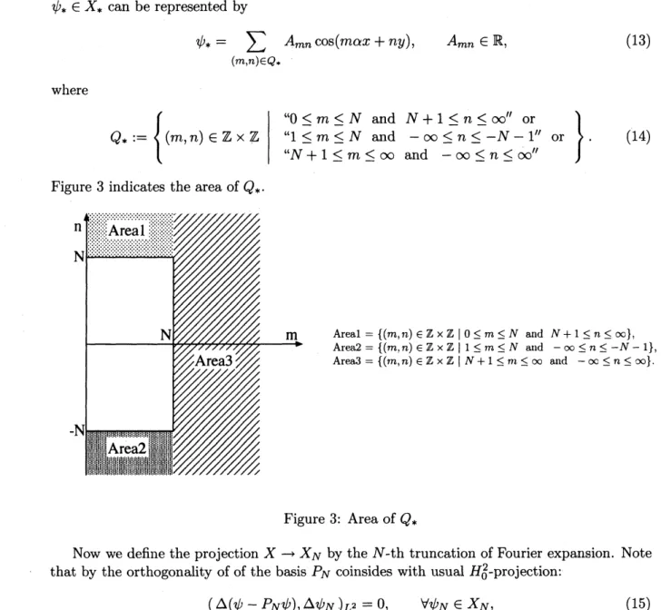
$Q_{*}:= \{(m, n)\in \mathbb{Z}\cross \mathbb{Z} (1\leq m\leq Nand0\leq m\leq NandN+1\leq m\leq\infty and-\infty\leq n\leq\infty\frac{N}{}\infty\leq n\leq-N-1"+1\leq n\leq\infty"or, or \}.$ (14)
Figure 3 indicates the
area
of$Q_{*}.$Areal$=\{(m, n)\in \mathbb{Z}\cross \mathbb{Z}|0\leq m\leq N$ and $N+1\leq n\leq\infty\},$
$A_{I}e_{c}’\iota 2=\{(m_{\}}n)\in \mathbb{Z}\cross \mathbb{Z}|1\leq m\leq NaIld-\infty\leq n\leq-N-1\},$
Area3 $=\{(m, n)\in \mathbb{Z}\cross \mathbb{Z}|N+1\leq m\leq\infty$ and $-\infty\leq n\leq\infty\}.$
Figure 3: Area of$Q_{*}$
Now we define the projection $Xarrow X_{N}$ by the N-th truncation of Fourier expansion. Note
that by the orthogonality ofofthe basis $P_{N}$ coinsides with usual $H_{0}^{2}$-projection:
$(\Delta(\psi-P_{N}\psi), \Delta\psi_{N})_{L^{2}}=0, \forall\psi_{N}\in X_{N}$, (15)
andwe obtain the following a priori
error
estimate for the liner problem of$\Delta^{2}\xi=g.$Lemma 4.1 For each $g\in X^{0}$ let $\xi\in X^{4}$ the solution of$\Delta^{2}\xi=g$, then
$\Vert\xi-P_{N}\xi\Vert_{X}\leq C_{5}\Vert g\Vert_{L^{2}}$
holds, where
5
Some
estimations
for
$X$Since
$|\psi|_{H^{3}(\Omega)}^{2}=\Vert u_{xxx}\Vert_{L^{2}}^{2}+3\Vert u_{xxy}\Vert_{L^{2}}^{2}+3\Vert u_{xyy}\Vert_{L^{2}}^{2}+\Vert u_{yyy}\Vert_{L^{2}}^{2}$
$= \frac{2\pi^{2}}{\alpha} \sum (\alpha^{6}m^{6}+3\alpha^{4}m^{4}n^{2}+3\alpha^{2}m^{2}n^{4}+n^{6})A_{mn}^{2}$
$(m,n)\in Q$
$= \frac{2\pi^{2}}{\alpha} \sum (\alpha^{2}m^{2}+n^{2})^{3}A_{mn}^{2},$
$(m,n)\in Q$
we have
(17)
Therefore since semi-norm $|\psi|_{H^{3}(\Omega)}$ becomes norm of $X$, we define the norm and the
inner-product of$X$ by
$\Vert\phi\Vert_{X}:=|\psi|_{H^{3}(\Omega)},$
$(u, v)_{X} :=(u_{xxx}, v_{xxx})_{L^{2}}+3(u_{xxy}, v_{xxy})_{L^{2}}+3(u_{xyy}, v_{xyy})_{L^{2}}+(u_{yyy}, v_{yyy})_{L^{2}},$
respectively.
For the norm $\Vert\cdot\Vert_{X}$, the following estimations hold.
Lemma 5.1 For any $\psi\in X$, and $\forall\psi_{*}\in X_{*}$, it can be checked that
$\Vert\psi\Vert_{L^{2}}\leq\alpha^{-3}\Vert\psi\Vert x, \Vert\psi_{*}\Vert_{L^{2}}\leq C_{1}\Vert\psi_{*}\Vert_{X},$
$\Vert\psi_{x}$
II
$L^{2}\leq\alpha^{-2}\Vert\psi\Vert_{X},$ $\Vert(\psi_{*})_{x}\Vert_{L^{2}}\leq C_{2}\Vert\psi_{*}\Vert_{X},$$\Vert\psi_{y}\Vert_{L^{2}}\leq C_{3}\Vert\psi\Vert_{X}, \Vert(\psi_{*})_{y}\Vert_{L^{2}}\leq C_{4}\Vert\psi_{*}\Vert_{X},$ $\Vert\nabla\psi\Vert_{L^{2}}\leq\alpha^{-2}\Vert\psi\Vert_{X}, \Vert\nabla\psi_{*}\Vert_{L^{2}}\leq C_{2}\Vert\psi_{*}\Vert_{X},$
$\Vert\nabla\psi_{x}\Vert_{L^{2}}\leq a^{-1}\Vert\psi\Vert_{X}, \Vert\nabla(\psi_{*})_{x}\Vert_{L^{2}}\leq C_{5}\Vert\psi_{*}||x,$
$\Vert\nabla\psi_{y}\Vert_{L^{2}}\leq C_{6}\Vert\psi\Vert_{X}, \Vert\nabla(\psi_{*})_{y}\Vert_{L^{2}}\leq C_{7}\Vert\psi_{*}\Vert_{X},$ $\Vert\triangle\psi\Vert_{L^{2}}\leq\alpha^{-1}\Vert\psi\Vert_{X}, \Vert\Delta\psi_{*}\Vert_{L^{2}}\leq C_{5}\Vert\psi_{*}\Vert_{X},$
$\Vert\triangle\psi_{x}\Vert_{L^{2}}\leq\Vert\psi\Vert x, \Vert\triangle(\psi_{*})_{x}\Vert_{L^{2}}\leq \Vert\psi_{*}\Vert_{X},$
$\Vert\Delta\psi_{y}\Vert_{L^{2}}\leq\Vert\psi\Vert_{X}, \Vert\triangle(\psi_{*})_{y}\Vert_{L^{2}}\leq \Vert\psi_{*}\Vert_{X},$
where
$C_{1}$ $=$ $\frac{1}{\alpha^{3}(N+1)^{3}},$ $C_{2}$ $=$ $\frac{1}{\alpha^{2}(N+1)^{2}},$
$C_{3}$ $=$ $\max\{1,$ $\frac{2\sqrt{3}}{9\alpha^{2}}\},$ $C_{4}$ $=$ $\max\{\frac{1}{(N+1)^{2}},9\alpha^{2}(N+1)^{2}2\sqrt{3}\},$
$C_{5}$ $=$ $\frac{1}{\alpha(N+1)},$ $C_{6}$ $=$ $\max\{1,$ $\frac{1}{2\alpha}\},$
$C_{7}$ $=$ $\max\{\frac{1}{N+1},$ $\frac{1}{2\alpha(N+1)}\}.$
Lemma 5.2 (Plum,1992 [7]) For any $\psi\in X$, the following assertion holds true:
$\Vert\psi\Vert_{L\infty}\leq C_{8}\Vert\psi\Vert_{L^{2}}+C_{9}\Vert\nabla\psi\Vert_{L^{2}}+C_{10}\Vert\Delta\psi\Vert_{L^{2}}$, (18)
where $\Vert\cdot\Vert_{L}\infty$ is the $\sup$-norm and
$C_{8}= \frac{\sqrt{\alpha}}{2\pi}, C_{9}=\frac{1.1548}{\sqrt{3}}\sqrt{\frac{\alpha^{2}+1}{\alpha}}, C_{10}=\pi\frac{0.44722}{3}\sqrt{\frac{9\alpha^{4}+10\alpha^{2}+9}{5\alpha^{3}}}.$
Lemma 5.1 and
Lemma
5.2 imply $L^{\infty}$-estimates immediately.Lemma 5.3 For $\forall\psi\in X$ and $\forall\psi_{*}\in X_{*}$, it is ture that
$\Vert\psi\Vert_{L\infty}\leq C_{11}\Vert\psi\Vert_{X}, \Vert\psi_{*}\Vert_{L}\infty\leq C_{12}\Vert\psi\Vert_{X},$
$\Vert\psi_{x}\Vert_{L}\infty\leq C_{13}||\psi\Vert_{X}, \Vert(\psi_{*})_{x}\Vert_{L}\infty\leq C_{14}\Vert\psi_{*}\Vert_{X},$
$\Vert\psi_{y}\Vert_{L}\infty\leq C_{15}\Vert\psi\Vert_{X}, \Vert(\psi_{*})_{y}\Vert_{L^{\infty}}\leq C_{16}\Vert\psi_{*}\Vert_{X},$
where
$C_{11} = a^{-3}C_{8}+a^{-2}C_{9}+\alpha^{-1}C_{10}, C_{12} = C_{1}C_{8}+C_{2}C_{9}+C_{5}C_{10},$ $C_{13} = \alpha^{-2}C_{8}+\alpha^{-1}C_{9}+C_{10}, C_{14} = C_{2}C_{8}+C_{5}C_{9}+C_{10},$ $C_{15} = C_{3}C_{8}+C_{6}C_{9}+C_{10}, C_{16} = C_{4}C_{8}+C_{7}C_{9}+C_{10}.$
We mention about partial integrations at finite-dimensional part. Let
$Y^{1} := \{v=\sum_{(m,n)\in Q}A_{mn}\sin(\alpha mx+ny)|A_{mn}\in \mathbb{R}, \Vert\nabla v\Vert_{L^{2}}<\infty\},$
then it holds true. Lemma 5.4
$(\psi_{x}, \phi)_{L^{2}}=-(\psi, \phi_{x})_{L^{2}}, \psi\in X^{1}, \phi\in Y^{1}.$ $(\psi_{y}, \phi)_{L^{2}}=-(\psi, \phi_{y})_{L^{2}}, \psi\in X^{1}, \phi\in Y^{1}.$
$(\Delta\psi, \phi)_{L^{2}}=(\psi, \Delta\phi)_{L^{2}}, \psi, \phi\in X^{2}.$
$(\triangle\psi, \Delta\phi)_{L^{2}}=(\Delta^{2}\psi, \phi)_{L^{2}}, \psi\in X^{4}, \phi\in X^{2}.$
$(J(u, v), w)_{L^{2}}=(J(w, u), v)_{L^{2}}=-(J(u, w), v)_{L^{2}}, u, v, w\in X^{2}.$
The following is an important propertyof Jacobian for (7).
Lemma 5.5 $\forall\psi_{1},$$\psi_{2}\in X^{1},$
$J(\psi_{1}, \psi_{2})\in X^{0},$
6
Verification
procedure
Thissection is devoted todetailed verification procedureofthesteady-state Kolmogorov
prob-lem (7).
6.1 Matrices
For fixed $\phi_{N}\in X_{N}$, define $H,$ $D,$$L,$ $G\in \mathbb{R}^{K\cross K}(1\leq i,j\leq K)$ by
$H_{ij}:=((\phi_{j})_{xxx}, (\phi_{i})_{xxx})_{L^{2}}+3((\phi_{j})_{xxy}, (\phi_{i})_{xxy})_{L^{2}}+$
$3((\phi_{j})_{xyy}, (\phi_{i})_{xyy})_{L^{2}}+((\phi_{j})_{yyy}, (\phi_{i})_{yyy})_{L^{2}}$, (19)
$D_{ij}:=(\triangle\phi_{j}, \triangle\phi_{i})_{L^{2}}$, (20)
$L_{ij}:=(\phi_{j}, \phi_{i})_{L^{2}}$, (21)
$G_{ij}:=(\triangle\phi_{j}, \Delta\phi_{i})_{L^{2}}+R(J(\phi_{N}, \Delta\phi_{j})+J(\phi_{j}, \Delta\phi_{N}), \phi_{i})_{L^{2}}$. (22)
6.2 Residual and fixed-point formulation
By setting
$r_{2N}:=-\triangle^{2}\phi_{N}-RJ(\phi_{N}, \triangle\phi_{N})-\cos y$, (23)
$r_{2N}$ is able tobe re-expandedas anelement in$X_{2N}$ and wecan computeits inner-productwith
$\{\phi_{i}\}_{i=1}^{K}$ and $L^{2}$-norm by interval arithmetic.
For fixed approximate solution $\phi_{N}\in X_{N}$ of (7), setting
$\phi=\phi_{N}+\psi$, (24)
we try to find residual term $\psi$
.
Substituting (24) to (7), we obtain a residual equation$\triangle^{2}\psi=-RJ(\phi_{N}+\psi, \Delta\phi_{N}+\triangle\psi)-\cos(y)-\triangle^{2}\phi_{N}$ in $T_{\alpha}$
.
(25)By denoting the right hand side of(25) by
$f(\psi):=-RJ(\phi_{N}+\psi, \triangle\phi_{N}+\triangle\psi)-\cos(y)-\Delta^{2}\phi_{N}$, (26)
from Lemma 5.5, $f$ : $Xarrow X^{0}$ is continuous and maps any bounded set of$X$ to a bounded set
of$X^{0}.$
Denote $F:=\triangle^{-2}f$ : $Xarrow X$, then $F$ becomes compact operator and problem (25) is
equivalent to afixed-point equation $\psi=F(\psi)$ in $X.$
6.2.1 Newton-like operator
By using the projection $P_{N}$, the fixed-point residual equation (25) can be decomposed into
finite-dimensional part $X_{N}$ and infinite-dimensional part $X_{*}$ as
$\{\begin{array}{l}P_{N}\psi = P_{N}F(\psi) ,(I-P_{N})\psi = (I-P_{N})F(\psi) .\end{array}$
Now we define Newton-like operator$\mathcal{N}_{N}$ : $Xarrow X_{N}$ by
and re-formulate the finite-dimensional part equivalently to
$P_{N}\psi=\mathcal{N}_{N}(\psi)$
.
Here $[I-F’[0]]_{N}^{-1}$ : $X_{N}arrow X_{N}$ is the inverse operator of $P_{N}(I-F’[O])$ : $Xarrow X_{N}$ whose
definition is restricted to $X_{N}$
.
Next we definie Newton-like operator $T$ on $X$ by$T(\psi):=\mathcal{N}_{N}(\psi)+(I-P_{N})F(\psi)$
which is the compact map.
6.2.2 Candidate set Let $\mathbb{I}\mathbb{R}$
be thesetof$K$-dimensional interval vector. A finite-dimensional set $U_{N}\subset X_{N}$ is taken
to bea set oflinear combinations of base functions in $X_{N}$ with interval coefficient $\{B_{i}\}_{1\leq i\leq K}$
such as
$U_{N}:= \sum_{i=1}^{K}B_{i}\phi_{i}$, (27)
where$B_{i}$ has upper andlower bounds suchthat $B_{i}=[\underline{B}_{i}, \overline{B}_{i}]$
.
Here$\sum_{i=1}^{K}B_{i}\phi_{i}$ isinterpretedastheset offunctions in which each element is linear combination of $\{\phi_{i}\}_{1\leq i\leq K}$ whose coefficient
of$\phi_{i}$ belongs to the corresponding interval $[\underline{B}_{i}, \overline{B}_{i}]$ for each $1\leq i\leq K$, namely,
$U_{N}= \{\sum_{i=1}^{K}v_{i}\phi_{i}\in X_{N} v_{i}\in \mathbb{R}, v_{i}\in B_{i}, 1\leq i\leq K\}$ . (28)
For $\alpha>0$, a infinite-dimensional set $U_{*}\subset X_{*}$ and a candidate set $U\subset X$ is taken to be
$U_{*}:=\{\psi_{*}\in X_{*}|\Vert\psi_{*}\Vert_{X}\leq\beta\}$, (29)
$U:=U_{N}+U_{*}$
.
(30)6.2.3 Verification condition
Theorem 6.1 Assume that the candidate set $U\subset X$ is defined by (29) and (27) with
(30), and that any element $\psi\in U$ is represented by
$\psi=\psi_{N}+\psi_{*}, \psi_{N}\in U_{N}, \psi_{*}\in U_{*}.$
Let $d=[d_{i}]\in \mathbb{I}\mathbb{R}^{K}$ denote an interval enclosure ofthe set whose i-th component consists
of
$\{(f(\psi)-f’[0]\psi_{N}, \phi_{i})_{L^{2}}\in \mathbb{R}|\psi\in U\}, 1\leq i\leq K$
.
(31)If, for an interval vector $v=[v_{i}]\in I\mathbb{R}^{K}$ enclosing the solution $x\subset \mathbb{I}\mathbb{R}^{K}$ for the
linear equation
$Gx=d$, (32)
theconditions
$v_{i}\subset B_{i}, 1\leq i\leq K$, (33)
and
$\psi\in$
Usup
$\Vert(I-P_{N})F(\psi)\Vert_{X}\leq\beta$ (34)
7
Some verification results
We use Sun Fortran 95 Ver.8.6 Linux-i386 (supporting interval arithmetic) and the inter-val arithmetic toolbox INTLAB [8] Version 6 with MATLAB
7.14.0.739
$(R2012a)$ on FujitsuPRIMERGY TX300 S5 (CPU: Intel Xeon E55202.$27GHz$, OS: Red Hat Enterprise Linux Server release 5.6).
In the case of$\alpha=0.7$, the basic flow (trivial solution) $-\cos(y)$ loses stability at a critical
Reynolds number $R_{c}$ and another steady state bifurcates. Okamoto-Shoji strongly suggested
that there is no secondary bifurcation from this branch. Nagatou [2] also enclosed the $R_{c}$ in
the interval [3.011528364444, 3.011528364446].
Figure 4 shows the bifurcation diagram, where $|A_{0,1}|$ means the absolute value of the
coef-ficient to the base $\cos(ny)$ for obtained approximate solution.
$|A_{0,1 ,\downarrow}|$
$arrow R$
Figure 4: Bifurcation diagram for $\alpha=0.7$
Figure 5 shows verification results for $R=3.015$, 3.02,3.05, 3.1,3.2, and 3.5 by IN-Linz.
We will report on various verification results for various a in another article.
Acknowledgments
This work was supported bya Grant-in-Aid from the Ministry ofEducation, Culture, Sports,
Science and Technology of Japan (No. 24340018).
References
[1] V.I. Iudovich, Exampleofthe generation of a secondary stationaryor periodic flow when
there is loss of stability of the laminar flow ofaviscous incompressiblefluid, J. Appl. Math.
Mech. 29 (1965) 527-544.
[2] K. Nagatou, A computer-assisted proofon the stability ofthe Kolmogorovflows of
incom-pressible viscous fluid, J. Comp. Appl. Math. 169 (2004) 33-44.
[3] M.T. Nakao, A numerical verification method for the existence ofweak solutions for
R$=3.015$ $\Vert\phi-\phi_{N}\Vert_{L}\infty\leq 2.0677\cross 10^{-11}$ R$=3.02$ $\Vert\phi-\phi_{N}\Vert_{L}\infty\leq 1.2599\cross 10^{-11}$ R $=3.05$ $\Vert\phi-\phi_{N}\Vert_{L}\infty\leq 9.8987\cross 10^{-12}$ R$=3.1$ $\Vert\phi-\phi_{N}\Vert_{L}\infty\leq 1.085610^{-11}$ R$=3.2$ $\Vert\phi-\phi_{N}\Vert_{L\infty}\leq 1.1318\cross 10^{-11}$ R$=3.5$ $\Vert\phi-\phi_{N}\Vert_{L^{\infty}}\leq 1.4785\cross 10^{-11}$
[4] M.T. Nakao, Y. Watanabe, N. Yamamoto, T. Nishida, and M-N. Kim, Computer assisted
proofsof bifurcating solutions fornonlinear heat convection problems, J. Sci. Comput. 43
(2010) 388-401.
[5] H. Okamoto and M. Shoji, Bifurcation diagrams in Kolmogorov’s problem of viscous
in-compressible fluid on 2-D flat tori, Japan J. Ind. Appl. Math. 10 (1993) 191-218.
[6] H. Okamoto, Mathematical Analysis
of
theNavier-StokesEquations (Japanese), UniversityofTokyo Press, 2009.
[7] M. Plum, Explicit$H_{2}$-estimates and pointwiseboundsforsolutions ofsecond-order elliptic
boundary value problems, J. Math. Anal. Appl. 165 (1992) 36-61.
[8] S.M. Rump, INTLAB –INTerval LABoratory, in Developments in Reliable
Com-puting, ed. T. Csendes, pp. 77-104, Kluwer Academic Publishers, Dordrecht, 1999.
http:$//www$
.
ti3. tu-harburg.$de/rump/$[9] Y. Watanabe, N. Yamamoto, M. T. Nakao and T. Nishida, A numerical verification of
nontrivial solutions for the heat convection problem, J. Math. Fluid Mech. 6 (2004) 1-20.
[10] Y. Watanabe, A computer-assisted proof for the Kolmogorov flows of incompressible
vis-cous fluid, J. Comp. Appl. Math. 223 (2009) 953-966.
[11] N. Yamamoto, A numerical verification method for solutions of boundary value problems
with local uniqueness by Banach’s fixed-point theorem, SIAMJ. Numer. Anal. 35 (1998)
2004-2013.
[12] N. Yamamoto, M.T. Nakao, and Y. Watanabe, A theorem for numerical verification on
local uniqueness of $s\dot{o}$lutions to fixed-point equations, Numer. Funct. Anal. Optim. 32

![Figure 2: Shape of the trivial solution $\phi=-\cos(y)$ and stream line of $[\phi_{y}, -\phi_{x}]^{T}.$](https://thumb-ap.123doks.com/thumbv2/123deta/5959207.1056251/3.892.93.793.127.546/figure-shape-trivial-solution-phi-cos-stream-line.webp)

![Figure 5: Shape of the stream line of $[(\phi_{N})_{y}, -(\phi_{N})_{x}]^{T}$ when $\alpha=0.7,$ N $=20.$](https://thumb-ap.123doks.com/thumbv2/123deta/5959207.1056251/11.892.219.765.112.1083/figure-shape-stream-line-phi-n-phi-alpha.webp)
