The Effects of Reversible Investment in the Presence of Business Cycle (Financial Modeling and Analysis)

The Effects

of Reversible Investment

in the Presence

of

Business Cycle1

大阪大学経済学研究科

₄

海溶(Haejun Jeon)

Graduate School of Economics

Osaka University

大阪大学・経済学研究科 西原 理 (Michi Nishihara)

Graduate School ofEconomics

Osaka University

1

Introduction

A framework of real options has been commonplace in corporate finance. The last thirtyyears,

following the monumental works of Brennan and Schwartz (1985) and McDonald and Siegel

(1986), have witnessed extensive debate and research onthe investment decision of a firm based

on the techniques of option pricing. Many attempts have been made in the framework of real options to broaden our horizons of understandingvarious issues in the real world. For instance,

a number of recent works emphasize the effect of business cycle on a firm’s investment and default decisions. Also, theproblemofunderinvestment and overinvestment induced by conflicts of interests has always been an essential issue to be investigated. Most research, however, has

examined those issues separately, and little is known about the interaction between them and

the joint determination ofcapital structure and investment decisions taking business cycle and debt maturity into account.

Inthe present paper, wepropose a model thatgives us acomprehensive understandingof the

essential issues that need to be integrated; theoptimalcapitalstructure,investment triggers, and default boundaryarejointly determined, taking businesscycle, debt maturity, and thevolatility

ofgrowth opportunitiesinto account.The firm optimallyswitches betweentwodiffusion regimes

paying switching costs, and the cash flow generated from the firm depends on the state of the economy, which switches via Markov chain. The optimal switching of diffusion regimes can be

read as the firm’s investment provided that the coefficients of

one

regime dominate those ofthe other. Furthermore, the modelintegratestheinvestment’sreversibility byallowing negative costs incurred when the firm switches from the regime with higher drift and volatility to that with

lower drift and volatility. It is naturalthat thetriggers ofinvestment, disinvestment, anddefault

depend onthe state ofthe economy, and those events

can

occur

not only by hitting the triggers

but also by exogenous change of the state of the economy. After illustrating the theoretical

framework, wepresent comparative statics regarding several parameters toarticulate the effects

1Thispaper is abbreviatedversionof Jeon and Nishihara (2014a), and was supportedbyKAKENHI 23310103,

26350424, 26285071, the Ishii Memorial Securities Research Promotion Foundation, and theJSPS Postdoctoral

Fellowship for ResearchAbroad. Thispaperwaswrittenwhen Michi Nishiharawas a JSPS PostdoctoralFellowfor

ResearchAbroad(Visiting Researcher at theSwiss FinanceInstitute,\’EcolePolytechniqueF\’ed\’eraledeLausanne).

Theauthors would like to thank theSwiss Finance Institute and the JSPS PostdoctoralFellowships forResearch

of business cycle, the volatility of growth opportunities, and the debt maturity structure. The results show that their effects are intimately linked witheach other, which clarifies the necessity

ofthe integrated framework for these issues.

In terms of theinfluenceofdebtstructure, the optimal leverage ratioincreasesin the maturity

of debtconsistently. Its effect ontheinvestment timing, however, is sharply distinguished by the

risks that thegrowth opportunities involve. When the firmcan raise the expected growth rate

without any incremental risks, the level of investment triggers is bimodal with respect to debt

maturity, peaking at each end, and is

more

sensitive when the investment is irreversible. This result is consistent with Diamond and He (2014), and can be construed in the context ofMyers

(1977); the well-known debt overhang problem. The author proposed to issue short-term debt

as a possible solution to mitigate the problem. Since the maturity ofgrowth opportunities is

infinityinourmodel in the sensethat the firmcan switch diffusionregimes anytime,shortening

debtmaturity correspondstoanydebt with finite maturity, andthus,the investmenttriggersget

lower

as

the debt maturity shortens to the moderate level. But the investment triggers rebound

as the maturity becomes very short, and this is because the optimal leverage ratio decreases

significantly, leading the triggers to the level of those of an all-equity firm. Thedisparity in the sensitivity depending on the reversibility of the investment is attributed to the fact that the

levered firm’s incentive to invest is stronger when it is reversible

so

that the triggers increase

less even though the maturity gets longer.

The resultis markedly different if the investment entails not only higher drift but also higher

volatility; the level of the investment triggers is unimodal with respect to the debt maturity,

and ismore sensitive when the investment is reversible. This resultcan be read in thecontext of Jensen and Meckling (1976). Equityholders usually have strong incentive to raise volatility at the

expense ofdebtholders. However, the portion ofrisks that equityholders shouldbearincreases

as

the debt maturity shortens to the moderate level, and thus the investment triggers rise. When the debt maturity becomes veryshort, however, the triggers decrease again for the

same reason

they increase in the previous

case.

The disparityof thesensitivity dependingon the investment reversibility is also ascribed to the fact that the levered firm’s incentive to invest is stronger

when it is reversible.

In terms of theeffects ofmacroeconomic condition,

we

present comparative staticsregarding

the persistence ofthe business cycle, and the results also differ significantly depending on the

volatility ofgrowth opportunities and the debt maturity. The level of investment triggers gets

lower consistently asrecessionshortens because of the increase inexpectedcash flow. Still, more

comprehensive understanding is needed regarding its effect on the optimal leverage ratio and

yield spreads. When the investment only raises the expected growth rate, the leverage ratio increases as recessionshortens because no further risks aretaken. The effect ismore significant for the firm with short-maturity debt, which can be read with the perspective of the negative

sensitivity ofthe investment triggerswith respect to the debt maturity. There is also difference

in the effects onyield spreads. When the debt is issued with long maturity, theyield spreads are more affected bythe increase in expected cash flow than the increase in leverage ratio, which is not significant for the debt with longmaturity, and thus the spreads decrease.

However, theresults aregreatly changed ifboth expected growthrate andvolatility increase

by the investment. Theoptimal leverage ratio doesnotincrease significantly, and it

even

sharply

decreases when the debt maturity is long enough and investment is reversible. This result can

be interpreted withthe perspectiveof thepositive sensitivity ofinvestment triggers with respect

to the debt maturity. As recession shortens, the timing of investment is pushed earlier by the

increase in expected cash flow, which implies that the firm is

more

likely to be

more

volatile. This issue is

more

significant for the firms with longer debt maturity and reversible investment

opportunities because the incentive of overinvestment is stronger for them, and thus they lower

the leverage ratio. The yield spreads of the debt with long maturity are more affected by the

expected cash flow, and thus they decrease as recession shortens. But, the debt with short

maturity is more likely to be affected by the increase in leverage ratio, and so the yield spreads tend to increase as recession shortens.

The remainder of this paperis organized as follows: The setup of the theoretical framework

is presented in Section 2.1, and the benchmark model which includes business cycle but does

not involve the investment opportunities is briefly introduced in Section 2.2. The main model that incorporates both exogenous shocks from macroeconomic condition and the investment opportunities isinvestigated inSection 2.3. The parameters adopted for the comparativestatics areintroduced inSection3.1, and the effects of the debt maturityand businesscycleareanalyzed in Section 3.2 and Section 3.3, respectively. The conclusion is given in Section 4,

2

The

model and solutions

2.1

Setup

Suppose that afirm’s assetvalue follows one-dimensional geometric Brownian motion, and that there exist two diffusion regimes in which the drift and diffusion coefficients differ. Then, the

dynamics of the asset value in each regime $i\in$

{H,L}

can be described as follows:

$dX_{t}=\mu_{i}X_{t}dt+\sigma_{i}X_{t}dW_{t}, X_{0}=x$, (2.1)

where $(W_{t})_{t\geq 0}$ is astandard Brownian motion defined on afiltered probabilityspace $(\Omega,$$\mathcal{F},$$\mathbb{F}=$ $(\mathcal{F}_{t})_{t\geq 0},$$\mathbb{P})$ satisfying theusual conditions. We postulate that the coefficients of regime$H$

domi-nate those of regime $L$ $($i.e. $\mu_{H}\geq\mu_{L}$ and $\sigma_{H}\geq\sigma L)$

.

All agents are assumedto be risk neutral,

and risk-free rate is given as a constant $r>\mu_{i}$ for $i\in$

{H,L}

to ensure that the firm value is

finite.

Following VathandPham (2007), wesupposethattheequityholders can switchthediffusion

regime, which involves switching costs. From the dominance of coefficients of diffusion regimes,

we can regard switching from regime $L$ to $H$ as

an

investment in production facilities, which

usually incurs positive

costs.2

Likewise, switching from regime $H$ to $L$ can be understood as a

switchofbusiness field that has fewer expected returnsbutis less volatile, whichusuallyinvolves

a liquidation ofa portion offacilities with negative

costs.3

In developing the analysis of the firm’s investment and default decision, the effect of the business cycle on them should not be ignored. Hence, we introduce the state of the economy denoted by $(\epsilon_{t})_{t\geq 0}$

.

It is independent of $(W_{t})_{t\geq 0}$, and its transition probabilityfollows a Poisson

law such that it is a two-state Markov chain switching between states $B$ and $R$, which refer to

boom and recession, respectively. Denoting the rate of leaving the state $k$ by $\lambda_{k}>0$, there is a

probability $\lambda_{k}\Delta t$ that the economy leaves the state $k$ in

an

infinitesimal time $\Delta t.$

Given the usual interpretation of business cycle, it is reasonable to suppose that the cash

flow, the investment costs, and the recovery rate dependon the businesscycle. Wesuppose that the firm with diffusion regime $i$ in the state $k$ generates cash flow at the rate of $\delta_{ik}X_{t}$ where $\delta_{ik}:=\delta_{i}\delta_{k}$ for $i\in$

{H,L}

and $k\in$

{B,R},

and it isnatural to

assume

that $\delta_{H}\geq\delta_{L}$ and $\delta_{B}\geq\delta_{R}.$ In terms of the switchingcosts, switchingfromregime$i$ to$j$ in the state $k$incurs aconstant cost

$\psi_{ik}$

.

The switching costs can be negative, and

$\psi_{ik}+\psi_{jk}>0$must holdto preventany redundant

switching.

Meanwhile, a firm can

use

debt financing, and the capital structure is determined by the trade-off between tax shields and bankruptcy costs. A constant tax rateis denoted by $\theta$

, and a

fraction $\gamma_{k}$ of asset value is lost when default

occurs

in the state $k\in$

{B,R}.

It is also natural

to presume $\gamma_{B}\leq\gamma_{R}$

.

Note that $\gamma_{k}$ needs to be interpreted in a broad sense; it incorporates

the huge losses accompanied with the default, such

as

the depreciation of the asset value, the damage of reputation, and the deterioration of credit availability in a simple form. Following Leland (1998) and Hackbarth, Miao, and Morellec (2006), we adopt stationary debt structure

with finite maturity. Namely, the firm issues debt with principal $p$, pays

a

coupon $c$constantly,

and rolls over a fraction $m$ of the total debt. The average maturity of the debt is $1/m$ if the

bankruptcy is neglected, and the debt structure is completely characterized bya tuple $(c, m,p)$

.

As usual, it is assumed that the debt is issued at par and the coupon ischosen to maximize the

firm value.

2.2

The

benchmark

model

Before entering into the main analysis, it might be useful for

us

to briefly introduce the

case

that does not involve the optimal switching ofdiffusionregimes

as a

benchmark model. That is,

the cash flow generated by the firm depends on the business cycle, but the firm does not have

theoption of investing in production facilities. This corresponds to the case with $\psi_{Lk}=\infty$ and

$\psi_{Hk}\geq 0$ for $k\in$

_{B,R},

_{and coincides with Hackbarth, Miao, and Morellec (2006).}

An unlevered firm’s value with diffusion regime $i$ and initial state $k$ is

as

follows:

$\overline{U}_{ik}(x):=\mathbb{E}[\int_{0}^{\infty}e^{-rt}(1-\theta)\delta_{ik}X_{t}dt|\epsilon_{0}=k],$ $i\in$

{H,L},

$k\in$

_{B,R},

(2.2)

where $X_{t}$ is the solution of (2.1). Since the state of the economy $(\epsilon_{t})_{t\geq 0}$ switches via a

two-state Markov chain, the firm value should satisfy the following system of ordinary differential

$3It$ _{is obvious that the equity holders will neverswitch from regime} $H$ to $L$ if_it incurs positive _{costs, which}

equations (ODEs) for$x\in(0, \infty)$ and $i\in$

{H,L}:

$(r+\lambda_{B})\overline{U}_{iB}(x)=\mathcal{L}_{i}\overline{U}_{iB}(x)+(1-\theta)\delta_{iB}x+\lambda_{B}\overline{U}_{iR}(x)$, (2.3) $(r+\lambda_{R})\overline{U}_{iR}(x)=\mathcal{L}_{i}\overline{U}_{iR}(x)+(1-\theta)\delta_{iR}x+\lambda_{R}\overline{U}_{iB}(x)$, (2.4)

where $\mathcal{L}_{i}$ is the generator of the diffusion process in regime $i\in$

{H,L}.

It is trivial to derive the

solutions of (2.3) and (2.4), and they can be found in the original paper, Jeon and Nishihara

(2014a).

The firm can use debt financing for the sake of tax $shields_{\}}$ but it involves the bankruptcy

costs, andthe default boundary is endogenously determined to maximize the interests of

equity-holders (e.g. Leland (1994), Leland and Toft (1996)). Taking cyclical cash flow into account, it is reasonable to conjecture that the default boundaryin recession is above that in boom, which

is verified from a numerical example in the following sections. Denoting the firm value and the

default boundarywith diffusionregime$i$ in the state $k$ by$\overline{V}_{ik}$ and$\overline{d}_{ik}$, respectively, the following

system ofODEs should be satisfied for $x\in(\overline{d}_{iR}, \infty)$ and $i\in$

{H,L}:

$(r+\lambda_{B})\overline{V}_{iB}=\mathcal{L}_{i}\overline{V}_{iB}(x)+(1-\theta)\delta_{iB}x+\theta c+\lambda_{B}\overline{V}_{iR}(x)$, (2.5) $(r+\lambda_{R})\overline{V}_{iR}=\mathcal{L}_{i}\overline{V}_{iR}(x)+(1-\theta)\delta_{iR}x+\theta c+\lambda_{R}\overline{V}_{iB}(x)$

.

(2.6)

For $x\in(d_{iB},$$d_{l}$ and $i\in$

{H,L},

the firm in boom will default when the state switches to recession by exogenous shocks, and the following ODE should hold:

$(r+\lambda_{B})\overline{V}_{iB}(x)=\mathcal{L}_{i}\overline{V}_{iB}(x)+(1-\theta)\delta_{iB^{X}}+\theta c+\lambda_{B}(1-\gamma_{R})\overline{U}_{iR}(x)$

.

(2.7)

By the same argument, the following system of ODEs should hold for the debt value for $i\in$

{H,L}:

$(r+m+\lambda_{B})\overline{D}_{iB}(x)=\mathcal{L}_{i}\overline{D}_{iB}(x)+c+mp+\lambda_{B}\overline{D}_{iR}(x) , x\in(d_{iR}, \infty)$, (2.8)

$(r+m+\lambda_{R})\overline{D}_{iR}(x)=\mathcal{L}_{i}\overline{D}_{iR}(x)+c+mp+\lambda_{R}\overline{D}_{iB}(x) , x\in(d_{iR}, \infty)$, (2.9)

$(r+m+\lambda_{B})\overline{D}_{iB}(x)=\mathcal{L}_{i}\overline{D}_{iB}(x)+c+mp+\lambda_{B}(1-\gamma_{R})\overline{U}_{iR}(x) , x\in(d_{iB}, d_{iR}].$ (2.10)

The solutions of theseequations can be found in the original paper, and weomit the derivation

for the same reason. Equity value is the firm value less the debt value in each regime and state

$($i.e. $\overline{E}_{ik}(x)=\overline{V}_{ik}(x)-\overline{D}_{ik}(x)$ for $i\in$

{H,L}

and $k\in\{B,R\})$. The default boundary and the

coefficients ofoption values aresimultaneously determinedbythe smooth-fit condition ofequity value and debt value at each trigger.

2.3

The main model

Having outlined the effects of the business cycle on the firm value, we shall now proceed to analyze the firm that has options to invest and disinvest. That is, now we suppose that the firm not only is affected by business cycle but also has options to switch the diffusion regime, which

incurs switching

costs.4

Asnoted earlier, equityholders have no incentive to switch from regime

$H$ to$L$ if it involves nonnegative costs, whichcorresponds to the case ofirreversible investment,

and for a moment we

assume

that the investment is reversible $(i.e. \psi_{Hk}<0 for k\in\{B,R\})$

_.

Before developing this argument regarding a levered firm, we shall briefly introduce the case of

the all-equity firm.

An increasing sequence of stopping times $(\tau_{n})_{n\geq 1}$ with $\tau_{n}\in \mathcal{T}$ and _{$\tau_{n}arrow\infty$} represents the decision when toswitch, and $(\iota_{n})_{n\geq 1}$ with $\iota_{n}\in$

{H,L}

denotes the regime at $\tau_{n}$ until$\tau_{n+1}$. Also, we define $I_{t}^{i}$

$:= \sum_{n\geq 0}\iota_{n}1_{[\tau_{n},\tau_{n+1})}(t)$ with $I_{0}^{i_{-}}=i$ to trace the regime value that began from

initial regime $i$

.

The process $(\epsilon_{t})_{t\geq 0}$ with _{$\epsilon_{0}=m$} is denoted by $\epsilon_{t}^{m}$

.

Given these notations, the

value ofan unlevered firm can be written as follows:

$U_{ik}(x) := \sup_{\tau_{n}\in \mathcal{T}}\mathbb{E}[\int_{0}^{\infty}e^{-rt}(1-\theta)\delta_{Ii\epsilon_{t}^{k}}X_{t}^{x,i}dt-\sum_{n=1}^{\infty}e^{-r\tau_{n}}\psi_{\iota_{n-1}\epsilon_{\tau_{n}}^{k}}]$, (2.11)

where $X_{t}^{x,i}$ is the solution of the controlleddiffusion process

$dX_{t}=\mu(X_{t}, I_{t}^{i})dt+\sigma(X_{t)}I_{t}^{i})dW_{t}, t\geq 0, X_{0}=x$

.

_(2.12)

It is natural to guess that the triggers of investment and disinvestment depend on the state of the economy, denoted by $s_{Lk}^{U}$ and $s_{Hk}^{U}$ for $k\in$

{B,R},

respectively. For

a

_moment, we suppose

that onlycash flow dependson the businesscycle. That is, for the sake of simplicity, we

assume

switching costs and recovery rate to be time-invariant. Given the cyclicality ofcash flow, it is obvious that $s_{iB}^{U}\leq s_{iR}^{U}$ holds for _$i\in$

{H,L}.

In other words, the investment is advanced and

disinvestment is delayed in boom in comparison with recession. Then, the value of all-equity firm with diffusion regime$L$ should satisfythefollowing system of ODEs for _{$x\in(O, s_{LB}^{U})$:}

$(r+\lambda_{B})U_{LB}(x)=\mathcal{L}_{L}U_{LB}(x)+(1-\theta)\delta_{LB}x+\lambda_{B}U_{LR}(x)$, _(2.13) $(r+\lambda_{R})U_{LR}(x)=\mathcal{L}_{L}U_{LR}(x)+(1-\theta)\delta_{LR}x+\lambda_{R}U_{LB}(x)$

.

(2.14)

Ifwe define $A:=U_{LB}-U_{LR}$ and $B:=\lambda_{R}U_{LB}+\lambda_{B}U_{LR}$, theycan be written

as

follows:

$(r+\lambda_{B}+\lambda_{R})A(x)=\mathcal{L}_{L}A(x)+(1-\theta)(\delta_{LB}-\delta_{LR})x$, (2.15)

$rB(x)=\mathcal{L}_{L}B(x)+(1-\theta)(\lambda_{R}\delta_{LB}+\lambda_{B}\delta_{LR})x$, (2.16)

and it is straightforward to calculate the solutions, which can be found in the original

paper.5

Given these solutions, the firm value of regime $L$ in $x\in(O, s_{LB}^{U})$ canbe written

as

follows:

$U_{LB}=(\lambda_{B}A+B)/(\lambda_{B}+\lambda_{R}) , U_{LR}=(B-\lambda_{R}A)/(\lambda_{B}+\lambda_{R})$

.

(2.17)

By the

same

argument, the firm of regime$H$ for $x\in(s_{HR}^{U}, \infty)$ can be obtained

as

follows:

$U_{HB}=(\lambda_{B}C+D)/(\lambda_{B}+\lambda_{R}) , U_{HR}=(D-\lambda_{R}C)/(\lambda_{B}+\lambda_{R})$, (2.18)

where$C$ and $D$ are given in the original paper.

For $x\in[s_{LB}^{U}, s_{LR}^{U})$, the firmofregime $L$ in recession will switch to regime $H$ when thestate

of the economy changes to boom, and thus the following ODE should hold:

$(r+\lambda_{R})U_{LR}(X)=\mathcal{L}_{L}U_{LR}(X)+(1-\theta)\delta_{LR^{X}}+\lambda_{R}(U_{HB}(X)-\psi_{LB})$ $($2.19$)$

Ageneralsolutionof$(r+\lambda_{R})U_{LR}(x)=\mathcal{L}_{L}U_{LR}(x)$ is $E_{1}x^{\alpha_{R}^{+}}+E_{2}x^{\alpha_{\overline{R}}}$

, and if we finda particular

solutionof (2.19), the general solution of (2.19) will be the sum of them. Having thesolution of

$U_{HB}$ in(2.18), we

can

guessthat the particular solutionisof theform$E_{3}x$ $E_{4}x$ $E_{5}x+E_{6},$

and a tedious algebra gives us the general solution as follows:

$U_{LR}(x)=E_{1}x^{\alpha_{R}^{+}}+E_{2}x^{\alpha_{\overline{R}}}+E_{3}x^{\beta_{BR}^{-}}+E_{4}x^{\beta^{-}}+E_{5}x+E_{6}$ _(2.20)

where the specific form of the functions $E_{3},$ $E_{4},$ $E_{5}$, and $E_{6}$ aregiven in the original paper.

Meanwhile, thefirm of regime $H$ with theasset value of$x\in(s_{HB}^{U}, s_{HR}^{U}$] will switch toregime

$L$, that is, liquidate a portion of its facilities, if the state of the economy changes to recession.

The

same

argument allows us to obtain the firm value

as

follows:

$U_{HB}(x)=F_{1}x^{\beta_{B}^{+}}+F_{2}x^{\beta_{B}^{-}}+F_{3}x^{\alpha_{BR}^{+}}+F_{4}x^{\alpha^{+}}+F_{5}x+F_{6}$_{, (2.21)}

where the specific form of the functions $F_{3},$ $F_{4},$ $F_{5}$, and $F_{6}$ can befound in original paper. In summary, the value of all-equity firm

can

be represented

as

follows:

$U_{LB}(x)=\{\begin{array}{ll}(\lambda_{B}A(x)+B(x))/(\lambda_{B}+\lambda_{R}) , x\in(0, s_{LB}^{U}) ,U_{HB}(x)-\psi_{LB}, x\in[s_{LB}^{U}, \infty) ,\end{array}$

$U_{LR}(x)=\{\begin{array}{ll}(B(x)-\lambda_{R}A(x))/(\lambda_{B}+\lambda_{R}) , x\in(0, s_{LB}^{U}) ,E_{1}x^{\alpha_{F\mathfrak{i}}^{+}}+E_{2}x^{\alpha_{\overline{R}}}+E_{3}x+E_{4_{\rangle}} x\in[s_{LB)}^{U}s_{LR}^{U}))U_{HR}(x)-\psi_{LR}, x\in[s_{LR\rangle}^{U}\infty))\end{array}$

$U_{HB}(x)=\{\begin{array}{ll}U_{LB}(x)-\psi_{HB}, x\in(0, s_{HB}^{U}],F_{1}x^{\beta_{B}^{+}}+F_{2}x^{\beta_{B^{-}}}+F_{3}x^{\alpha_{BR}^{+}}+F_{4}x^{\alpha^{+}}+F_{5}x+F_{6}, x\in(s_{HB}^{U}, s_{HR}^{U}],(\lambda_{B}C(x)+D(x))/(\lambda_{B}+\lambda_{R}) , x\in(s_{HR}^{U}, \infty) ,\end{array}$

$U_{HR}(x)=\{\begin{array}{ll}U_{LR}(x)-\psi_{HR}, x\in(0, s_{HR}^{U}],(D(x)-\lambda_{R}C(x))/(\lambda_{B}+\lambda_{R}) , x\in(s_{HR}^{U}, \infty) .\end{array}$

The constant coefficients and the triggers are simultaneously determined by smooth-fit

con-ditions at each trigger. Even if we allow cyclicality to switching costs and recovery rate, the

solutioncan beobtainedby thesame argument, except that the inequality regardingthelevel of

switching triggers might be changed. For brevity, thedetailed illustration regarding those cases

is omitted here.

Having discussed the

case

of

an

all-equity firm so far, we shall now proceed to analyzing

a

levered firm. Provided that theinvestment is reversible $(i.e. \psi_{Hk}<0 for k\in\{B,R\})$, thedefault

occurs

in regime $L$ only. The rationale behind this result is as follows: if disinvestment involves

negative costs, equityholders of the firm in regime $H$ will switch to regime $L$ right before the

default rather than default in regime $H$, unless the covenant prohibits liquidating production

facilities.

Now we have triggers ofinvestment, disinvestment, and default in each state $k$, denoted by

$s_{Lk},$ $s_{Hk}$, and $d_{Lk}$, respectively, for $k\in$

{B,R}.

If we only allow the cyclicality to the cash flow

forthe sake of simplicity, as assumed in theprevious analysis, we

can

conjecture that alltriggers

flow, and this is verified by a numerical example in the following sections. It is natural that the disinvestment triggers decrease as the reversibility of investment worsens (i.e. as $\psi_{Hk}(<0)$

increases for $k\in\{B,R\}$), and they can

even

be located below the default triggers. If this is the

case, the firm would switch to regime $L$ right before the default, but

we assume

for

a

moment

that the reversibility is high enough that we can have the following inequality for the level of thresholds: $d_{LB}<d_{LR}<s_{HB}<s_{HR}<s_{LB}<s_{LR}.$

The technique used to calculate the firm value is similar to the case of the all-equity firm

except that the firm defaults. The firm value of diffusion regimes $L$ and $H$ for _{$x\in(d_{LR}, s_{LR})$}

and $x\in(s_{HB}, \infty)$, respectively, can be obtained by the same argument used in (2.17), (2.18),

(2.19), and (2.21).

For $x\in(d_{LB}, d_{LR}]$, the firm in boom will default ifthe state switches to recession, and the

following ODE should hold:

$(r+\lambda_{B})V_{LB}(x)=\mathcal{L}_{L}V_{LB}(x)+(1-\theta)\delta_{LB}x+\thetac+\lambda_{B}(1-\gamma_{R})U_{LR}(x)$

.

(2.22)

A general solution of $(r+\lambda_{B})V_{LB}(x)=\mathcal{L}_{L}V_{LB}(x)$ is $L_{1}x^{\alpha_{B}^{+}}+L_{2}x^{\alpha_{B}}$, and if

we

find

a

particular solution of (2.22), then the general solution of (2.22) is the sum of them. Having the all-equity

firm value in (2.17), we can calculate the solution as follows:

$V_{LR}(x)=L_{1}x^{\alpha_{R}^{+}}+L_{2}x^{\alpha_{\overline{R}}}+L_{3}x^{\beta_{BR}^{-}}+L_{4}x^{\beta^{-\fbox{Error::0x0000}}}+L_{5}x+L_{6}$ _(2.23)

where thespecific form ofthe functions $L_{3},$ $L_{4},$ $L_{5}$, and $L_{6}$

are

given in theoriginal paper.

Insummary, the value ofalevered firmcan be represented as follows:

$V_{LB}(x)=\{\begin{array}{ll}(1-\gamma_{B})U_{LB}(x) , x\in(0, d_{LB}],L_{1}x^{\alpha_{B}^{+}}+L_{2}x^{\alpha_{B}}+L_{3}x^{\alpha_{BR}^{+}}+L_{4}x^{\alpha^{+}}+L_{5}x+L_{6}, x\in(d_{LB},d_{LR}],(\lambda_{B}G(x)+H(x))/(\lambda_{B}+\lambda_{R}) , x\in(d_{LR}, s_{LB}) ,V_{HB}(x)-\psi_{LB}, x\in[s_{LB}, \infty)\end{array}$

$V_{LR}(x)=\{\begin{array}{ll}(1-\gamma_{R})U_{LR}(x) , x\in(0,d_{LR}])(H(x)-\lambda_{R}G(x))/(\lambda_{B}+\lambda_{R})) x\in(d_{LR}, s_{LB}) ,K_{1}x^{\alpha_{R}^{+}}+K_{2}x^{\alpha_{\overline{R}}}+K_{3}x^{\beta_{BR}^{-}}+K_{4}x^{\beta^{-}}+K_{5}x+K_{6}, x\in[s_{LB}, s_{LR}) ,V_{HR}(x)-\psi_{LR)} x\in[s_{LR}, \infty)\end{array}$

$V_{HB}(x)=\{\begin{array}{ll}V_{LB}(x)-\psi_{HB}, x\in(0, s_{HB}],M_{1}x^{\beta_{B}^{+}}+M_{2}x^{\beta_{B}^{-}}+M_{3}x^{\alpha_{BR}^{+}}+M_{4}x^{\alpha_{BR}}+M_{5}x^{\alpha^{+}}+M_{6}x^{\alpha^{-}}+M_{7}x+M_{8}, x\in(s_{HB}, s_{HR}],(\lambda_{B}I(x)+J(x))/(\lambda_{B}+\lambda_{R}) , x\in(s_{HR}, \infty) ,\end{array}$

$V_{HR}(x)=\{\begin{array}{ll}V_{LR}(x)-\psi_{HR}, x\in(0, s_{HR}])(J(x)-\lambda_{R}I(x))/(\lambda_{B}+\lambda_{R})) x\in(s_{HR}, \infty) .\end{array}$

The functional formof the coefficients above can be found in the original paper.

ODEs:

$(r+m+\lambda_{B})D_{LB}(x)=\mathcal{L}_{L}D_{LB}(x)+c+mp+\lambda_{B}D_{LR}(x) ,x\in(d_{LR}, s_{LB})$,

$(r+m+\lambda_{R})D_{LR}(x)=\mathcal{L}_{L}D_{LR}(x)+c+mp+\lambda_{R}D_{LB}(x) ,x\in(d_{LR}, s_{LB})$, $(r+m+\lambda_{B})D_{LB}(x)=\mathcal{L}_{L}D_{LB}(x)+c+mp+\lambda_{B}(1-\gamma_{R})U_{LR}(x) , x\in(d_{LB}, d_{LR}],$

$(r+m+\lambda_{R})D_{LR}(x)=\mathcal{L}_{L}D_{LR}(x)+c+mp+\lambda_{R}D_{HB}(x) ,x\in[\mathcal{S}_{LB}, s_{LR})$,

$(r+m+\lambda_{B})D_{HB}(x)=\mathcal{L}_{H}D_{HB}(x)+c+mp+\lambda_{B}D_{HR}(x) ,x\in(s_{HR}, \infty)$,

$(r+m+\lambda_{R})D_{HR}(x)=\mathcal{L}_{H}D_{HR}(x)+c+mp+\lambda_{R}D_{HB}(x) ,x\in(s_{HR_{\rangle}}\infty)$,

$(r+m+\lambda_{B})D_{HB}(x)=\mathcal{L}_{H}D_{HB}(x)+c+mp+\lambda_{B}D_{LR}(x) ,x\in(s_{HB}, s_{HR}].$

The solutions can be acquired in the same manner, and they can be summarized as follows:

$D_{LB}(x)=\{\begin{array}{ll}(1-\gamma_{B})U_{LB}(x) , x\in(0, d_{LB}],S_{1}x^{\alpha_{mB}^{+}}+S_{2}x^{\alpha_{\overline{m}B}}+S_{3}x^{\alpha_{BR}^{+}}+S_{4}x^{\alpha^{+}}+S_{5}x+S_{6}, x\in(d_{LB}, d_{LR}],(\lambda_{B}N(x)+O(x))/(\lambda_{B}+\lambda_{R}) , x\in(d_{LR}, s_{LB}],D_{HB}(x) , x\in(s_{LB)}\infty)\end{array}$

$D_{LR}(x)=\{\begin{array}{ll}(1-\gamma_{R})U_{LR}(x) , x\in(0, d_{LR}])(O(x)-\lambda_{R}N(x))/(\lambda_{B}+\lambda_{R}) , x\in(d_{LR}, s_{LB}],R_{1}x^{\alpha_{mR}^{+}}+R_{2}x^{\alpha_{\overline{m}R}}+R_{3}x^{\beta_{mBR}^{-}}+R_{4}x^{\beta_{m}^{-}}+R_{5}, x\in(s_{LB}, s_{LR}],D_{HR}(x) , x\in(s_{LR}, \infty) ,\end{array}$

$D_{HB}(x)=\{\begin{array}{ll}D_{LB}(x) , x\in(0, s_{HB}],T_{1}x^{\beta_{mB}^{+}}+T_{2}x^{\beta_{mB}^{-}}+T_{3}x^{\alpha_{mBR}^{+}}+T_{4}x^{\alpha_{\overline{m}BR}}+T_{5}x^{\alpha_{m}^{+}}+T_{6}x^{\alpha_{\overline{m}}}+T_{7}, x\in(s_{HB}, s_{HI\mathfrak{i}}],(\lambda_{B}P(x)+Q(x))/(\lambda_{B}+\lambda_{f} x\in(s_{HR}, \infty) ,\end{array}$

$D_{HR}(x)=\{\begin{array}{ll}D_{LR}(x) , x\in(0, s_{HR}],(Q(x)-\lambda_{R}P(x))/(\lambda_{B}+\lambda_{R}) , x\in(s_{HR}, \infty) .\end{array}$

The functional form ofthe coefficients above can be found in the original paper.

Equity valueis the firm value less the debt value (i.e. $E_{ik}(x)=V_{ik}(x)-D_{ik}(x)$ for $i\in$

{H,L}

and $k\in\{B,R\})$

.

The triggersand the coefficients of option values aresimultaneously determined

by the smooth-fit conditions of equity value and debt value at each trigger.

The solutions can beobtained bythesame argument evenifwe allow cyclicality to switching

costs andrecoveryrateexcept that theinequalityregarding the leveloftriggers may be changed, and the illustrationfor those

cases

is omitted to avoid unnecessary duplication.

As noted earlier, the firm will not switch back to regime $L$ if $\psi_{Hk}\geq 0$ for $k\in$

{B,R},

and

this corresponds to the

case

of irreversible investment. Ifthe investment is indeed irreversible,

there

are no

disinvestmenttriggers, andthe default

can

also

occur

in regime $H$, but thedefault

boundaries of regime $H$ will be lower than those of regime L. The triggers of investment and

default are denoted by $\hat{s}_{Lk}$ and $\hat{d}_{ik}$

for each regime $i\in$

{H,L}

and state $k\in$

{B,R}.

The firm

value, debt value, and equity value are denoted by $\hat{V}_{ik},$ $\hat{D}_{ik}$, and $\hat{E}_{ik}$, respectively. Regarding an

unleveredfirm,theinvestment triggerandthe firm value

are

denotedby$\hat{s}_{Lk}^{U}$and$\hat{U}_{ik}$

,respectively.

3

Comparative

statics

3.1

Parameters

We adopt $r=0.08$

_as

aconstant risk-free rate, which is close to the historical average Treasury rates (e.g.Huang and Huang (2012)). Forthe diffusion regimes, it is assumedthatthecoefficients of regime $H$ dominate those of regime $L$, and we adopt _{$\mu_{L}=0.2$} and _{$\mu_{H}=0.3$} for the drift

coeffients. Regarding the diffusion coefficients, we fix $\sigma L=0.2$ and analyze with respect to

different volatilities of regime$H$toclarify the individual features of growthopportunities,namely,

$\sigma H=0.2$ and $\sigma H=0.25$

.

Compared with the former in which only the expected growth rate

grows, in the latter case, it is accompanied by the increase of risks.

For simplicity, we postulate that only cash flow differs depending on business cycle. That

is, switching costs and recovery rateare assumed to be

time-invariant.6

Since it is natural that

more

cash flow is generated in boom than in recession,

we

presume that $\delta_{B}=1.5$ and $\delta_{R}=1,$

having $\delta_{H}=\delta_{L}=0.06$ fixed

as

Huang and Huang (2012)

did.7

We adopt $\gamma_{B}=\gamma_{R}=0.4869$

for afraction of loss at default to reflect that the average recovery rate is 51.31% in Huang and Huang (2012).

In terms of switching costs, we shall limit ourselves to investment with high reversibility,

namely $\psi_{LB}=\psi_{LR}=15$ and $\psi_{HB}=\psi_{HR}=-14$,

so

thatwe

can

verify the inequality regarding

the level of thresholds assumed in the previous section (i.e. $d_{LB}<d_{LR}<SHB<SHR<SLB<$

$sLR)$

.

Ifthe reversibility ofinvestment worsens, the disinvestment _triggers

can

_belocated _below

the default boundaries, which implies that the firm will disinvest right before the default. This is the extreme

case

of the agency

problem,8

which is not the main issue of the present paper, and we shall focus

on

other aspects of the problem.

Following Hackbarth, Miao, and Morellec (2006),

we

adopt $\lambda_{B}=0.1$ and $\lambda_{R}=0.15$ for the

persistenceof the business cycle, and $m=0.2$ fortherate of rollover (i.e. 5 yearsofaveragedebt

maturity). For the tax rate, we

use

$\theta=0.35$

as numerous

works have done _(e.g. Leland (1994),

Leland and Toft (1996)). Initial asset value is assumed to be $x_{0}=100.$

3.2

The debt

maturity

In thissubsection,

we

let $m$ (therate ofrollover) vary and examine the impact of debt maturity

on theoptimal leverage and investment decisions of the firm. As notedearlier, the debtis issued

at parand thecoupon is chosen tomaximize the firm value.

First, we assume that the firm

can

raise the expected growth rate via growth opportunities

without any increase of volatility $(i.e. \sigma H=\sigma_{L}=0.2)$. $6$

Hackbarth, Miao, and Morellec (2006) also assumed that the recovery rate is irrelevant to business cycle.

Refer toElliott,Miao, and Yu (2009), Du and MacKay (2010), and Jeon and Nishihara(2014c) for theimpact of

time-varying switching costsonthe investment decisions ofa firm.

7Theyassumedthat thepayoutratio is fixed at 6%regardlessof the creditratings.

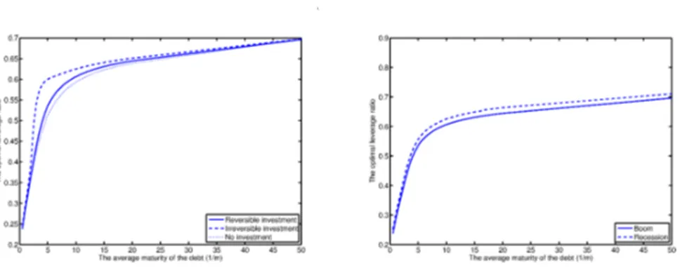
Figure 1: The optimal leverage ratio w.r.$t$

.

debt maturity provided _{$\sigma H=\sigma_{L}=0.2$} Panel (a) ofFigure 1 presents thefirm’s optimal leverage fordifferent investmentreversibility provided that the firm is ofregime $L$ and there is

an

upturn in the economy. We

can see

that

the optimal leverage increases in the debt maturity, which is in line with Leland and Toft

(1996), Leland (1998), and Hackbarth, Miao, and Morellec $($2006$)^{}$ The reason for this result is

delineated in Hackbarth, Miao, and Morellec (2006) as follows: a reduction in the maturity of the debt contract implies

an

increase in the debt service, which increases thedefault probability, and thus the optimal response of the firm is to lower the leverage ratio. We

can

also notice that the leverage ratio of the firmwith reversible investment is lower than that of the firm with irreversible investment. Panel (b) ofFigure 1 shows the countercyclical leverage ratio, which is consistent with Hackbarth, Miao, and Morellec (2006) and Chen and Manso (2010).

(a) Reversible/Investment (b) Reversible/Disinvestment (c) Irreversible/Investment

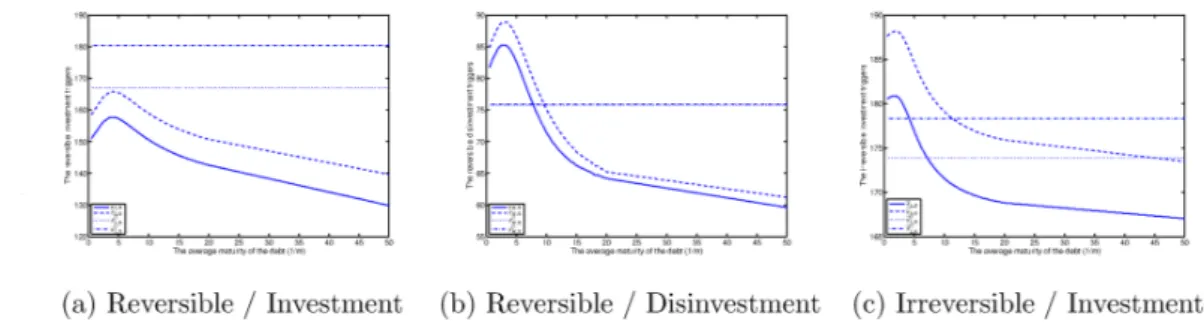
Figure 2: The level of the triggers w.r.$t$. debt maturity provided$\sigma_{H}=\sigma_{L}=0.2$

Figure 2 describes the investment triggers of the firm with reversible and irreversible

invest-ment opportunities. We can see that the triggers are bimodalwith respect tothedebt maturity,

peaking at each end, and

more

sensitive when the investment is irreversible. This result is

con-sistent with Diamond and He (2014), which elucidates theeffects of debt maturity, and can be

construed in the context of Myers (1977): the underinvestment problemwith risky debt

financ-ing. Myers (1977) says that ifdebt matures after the expiration of the investment option, risky

debt financing mayinduce theincentive of underinvestment because aportion of equityholders’

benefits accrue to thedebtholdersin the form ofreductionofthe default probability; to mitigate

this problem, the author suggested shortening debt maturity.

9InBrennan andSchwartz (1978), the optimal leverage decreasesasthe maturity gets longer, but thedefault

Inour model, thematurity ofthe options is infinity in the sense that the firm

can

invest in production facilities any time, and

so

shorteningof debt maturity corresponds to any debt with finite maturity. We can see in Figure 2 that the investment triggers get lower

as

the average

debt maturity shortens from infinity to the moderate level. As thematuritybecomes veryshort,

however, they rebound; and this result is intimately linked with Figure 1. As the debt maturity

shortens, the optimal leverage decreases significantly (from 70% to 25% in the range of our

analysis), and thus the level of investment triggers converges to that of anunlevered firm asthe

debt maturitybecomes very short. It

seems

that thisexplication does not fitverywellifonlythe

reversible investment triggers are concerned. But, the tendency for the triggers to converge to

those ofan all-equity flrmiscrystal clear inthedisinvestment triggers andirreversible investment

triggers. The disparity of thedegree of convergence andsensitivity is attributed tothe fact that

the incentive ofinvestment ofa leveredfirm is strongerwhen it isreversible

so

that thetriggers

increase less

even

though the maturity gets longer.

Now we shall proceed to the case in which the investment is accompanied by not only the

increase ofexpected growth rate butalsothe increase ofvolatility $($i.e. $\sigma_{H}=0.25$ and $\sigma L=0.2)$

.

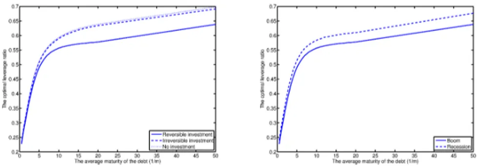
Figure 3: The optimal leverage ratio w.r.$t$

.

debt maturity provided _{$\sigma_{H}=0.25>\sigma L=0.2$}

We

can see

from Panel (a) of Figure 3 that the optimal leverage ratio also increases in debt

maturity regardless of the increase ofrisks viagrowth opportunities. Furthermore, the negative correlation between the growth opportunities and leverage ratio is moresignificant; the leverage ratio of the firm with reversible investment is lower than that with irreversible investment and

even that with no real

options.10

Note that the gap between them decreases as the maturity of

debt shortens. The countercyclicality ofleverage ratio is also shown in Panel (b) of Figure 3,

and the gap between the optimal leverage ratio in each state widens

as

thevolatility of growth opportunity increases.

We alsohave similar results regarding the investment reversibility and the capital structure. The leverage ratio with reversible investment is lower than that with the irreversible one, even

lower than the case with no investment. Yet, the rationale behind this result is different from

that in Figure 1. The investment raises not onlytheexpected growth rate but also the volatility,

and this makes the equity holders with reversible investment opportunity advance thetimingof

$1\fbox{Error::0x0000}$

hasbeen examined innumerousworks that there is negativecorrelation betweenleverageratio and growth

investment to earlier than those with irreversible one. This implies that the firm is more likely

to be volatile, leaving less room for raising the leverage

ratio.11

$1\infty$ $\xi$

$1^{\vee-}t\infty--\cdot f_{\mu}\fbox{Error::0x0000}ae_{0^{\vee^{\backslash }}5}:i0(\cdot 1\mathfrak{d}\sim\cdot un..mt:_{m^{\mathfrak{N}}} \nu/\cdot\cdot u(i/n)0s\infty$

(a) Reversible/Investment (b) Reversible/Disinvestment (c) Irreversible/Investment

Figure 4: The level of the triggers w.r.$t$. debt maturity provided $\sigma_{H}=0.25>\sigma_{L}=0.2$

Meanwhile, Figure 4 shows that the investment triggers are unimodal with respect to the

debt maturity andmoresensitivewhentheinvestment isreversible, contrastingsharplywith the

result from Figure 2. This result is directly linked to the overinvestment problem (e.g. Jensen and Meckling (1976)). When the maturity of both the real options and the debt is infinity,

equityholders have a strongincentive to raise volatility, because their expected profits increase

at the expense of debtholders. Yet, the portion ofrisks that equityholders shouldbear increases as the debt maturity shortens, and thus the investment triggers increase. When the maturity

becomes very short, however, the triggers decrease again for the

same reason

they increase in

Figure 2; namely, the optimal leverage ratio decreases $significantly_{\rangle}$ and thus the triggers tend

to converge to the level of those of an all-equity firm. The disparity of the convergence and the sensitivity is also ascribed to the fact that the incentive of the investment of a levered

firm is stronger whenit is reversible. This sharp contrast in the effects of growth opportunities

on investment timing is a novel result; this result is not presented in Diamond and He (2014)

because only thedrift is controlled via the investment in their model.

3.3

The persistence of business cycle

In this subsection, we examine how the business cycle affects a firm’s decisions to invest and

default. Having in the previoussubsection discussed the significant effects of debt maturity and

the volatility of growth opportunities on a firm’s the optimal leverage ratio and investment

decision,

we

finditnaturalto conjecture that thereexist

a

disparity in the effectsofthebusiness

cycle which depends on them. Hence, we present the comparative statics of$\lambda_{k}$ with respect to

thedifferent investment projects anddebtmaturity; namely, for$\sigma_{H}=0.2$and$\sigma H=0.25$, and for

$m=0.2$ (a bond with average maturityof 5 years) and $m=0$ (aconsol bond),

respectively.12

llThisrationale canalso be confirmed by Figure4 whichpresentsthe level of investment triggers, that is, the

incentive to invest. We can see that the gap between the leverage ratiosofthetwocases widens as theaverage

maturityofthe debt lengthenssothat thedifference between the investment timingof them increases.

12Theyare chosento represent short and long maturity. When the maturity becomesveryshort (e.g.6months),

the yield spreads andtheleverageratioareverylow, unsuitablefor analyzing the effects, andso weadopt$m=0.2$

Note that there is

a

probability $\lambda_{k}\Delta t$ that the economy leave the state $k$ in

an

infinitesimal

time $\triangle t$

, and thus the state $k$ shortens

as

$\lambda_{k}$ increases for $k\in$

_{B,R}.

The

same

_argument can

be obtained from the comparative statics of$\lambda_{B}$ and $\lambda_{R}$, and for brevity we introduce only the

latter.

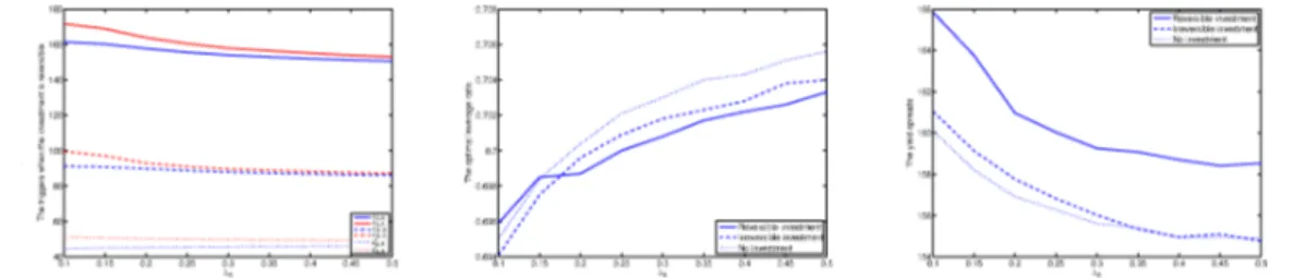
Figure 5: The various triggers, the optimal leverage ratio, and the yield spreads provided $\sigma H=$

$\sigma_{L}=0.2$ and _$m=0.2$

Figure 6: The various triggers, the optimal leverage ratio, and the yield spreads provided$\sigma H=$

$\sigma_{L}=0.2$ and $m=0$

First, we supose that the firm can raise the expected growth rate without increasing risks at all $(i.e. \sigma H=\sigma L=0.2)$

.

Figures 5 and 6 correspond to the _{comparative statics of} $\lambda_{R}$ with

$m=0.2$ and $m=0$, respectively. It is assumed that the firm’s asset value is of regime $L$ and

the economy is in an upturn. Above all, we

can

observe in Panel (a) of Figure 5 and 6 that the investment gets earlier as $\lambda_{R}$ increases, and this is because the expected cash flow increases as

the recession shortens. Also, the gap between triggers of each state diminishes

as

thepersistence

of thestate shortens.

In terms of theoptimal leverageratio, we

can see

that it increases in$\lambda_{R}$because the expected

cash flowincreases without any incremental risks. It is moresignificant for the firm with

short-maturity debt $(i.e. m=0.2)$, and this

can

be read in the context of what we have examined

in the previous _{subsection: the negative sensitivity of investment triggers with respect to debt}

maturity (providedthat it is not very short) in Figure 2. Theincentive of investment is stronger when the debt is issued with short maturity, because the underinvestment problem noted in Myers (1977) is mitigated.

The effects on yield spreads also differ depending on the debt structure. When the debt

is issued with long maturity, the yield spreads are

more

affected by the increase in expected

cash flow than the leverage ratio, which does not increase significantly, and thus the yield

with short maturity, and thus the yield spreads tend to increase as recession shortens. With

irreversible investment, they sharply increase and then decrease gradually, and this result can

also be construed with what wehave discussed in the previous subsection; the sensitivity of the

triggers is more evident whenthe investment is irreversible. Thus, the asset value is more likely

to have higher drift when the investment is irreversible, leading to the gradual decrease in the yield spreads, $0\cdot a$ $0\cdot Z$ $\xi_{0\infty}^{0\cdot t}\not\in^{0\cdot t}.$ 沖 $0\cdot\aleph_{7}\mathfrak{d}I,$ 。1023 $0.$ $0.$

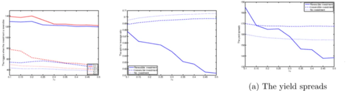
Figure 7: The various triggers, the optimalleverage ratio, and the yield spreads provided $\sigma_{H}=$

$0.25>\sigma L=0.2$ and $m=0.2$

(a) The yield spreads

Figure 8: The various triggers, the optimal leverage ratio, and the yield spreads provided $\sigma_{H}=$ $0.25>\sigma_{L}=0.2$ _and $m=0$

Now we shall proceed to the case in which the higher expected growth rate entails higher volatility $($i.e. $\sigma_{H}=0.25$ and $\sigma_{L}=0.2)$

.

Figures 7 and 8 correspond to the comparative statics

of $\lambda_{R}$ with $m=0.2$ and $m=0$, respectively. As observed earlier, the investment timing gets

advanced and the gap between triggers of each state decreases as $\lambda_{R}$ increases, but the other

issues make a sharp distiction from the former analysis.

The optimal leverage ratio tends to increase in $\lambda_{R}$ for most

cases

because of the increase

in the expected cash flow. It sharply decreases, however, for the firm with

a

consol bond and

reversible investment opportunities, and this can also be read in the context of the analysis

in the previous subsection: the negative sensitivity ofinvestment triggers with respect to debt

maturity (provided that it is not very short) in Figure 4. As the expected cash flow increases,

the investment timing gets earlier; that is, the firm is

more

likely to be more volatile, and this issue is moresignificant for the firms with longer debt maturityand reversible investment oppor-tunities because the incentive of overinvestment is stronger for them. Note that the sensitivity ofinvestment triggers is more significant when the investment is reversible.

Theeffects

on

yield spreads also differ depending

on

the maturityof debt. Theyield spreads decrease in $\lambda_{R}$ providedthat thedebt is issued with long maturity, and theyaremost significant

when the investment is reversible. It is obvious for the

case

ofreversible investment, because in

that case the leverage ratio sharply decreases and the expected cash flow increases. The yield

spreads also decrease in other two

cases

(i.e. the cases with irreversible investment and no real

options) because the effect of increase in expected cash flow is more significant for the debt

with longer maturity and the increase ofleverageis not significant. However,this isnot the

case

when the debt is issued with short maturity. The debt value is less affected by the increase in expected cash flow, and

so

the yield spreads increasesifthe investment is irreversibleor if there

is noswitching indiffusionregime. Whentheinvestment is reversible, the yield spreads decrease

because thechange in leverage ratio is less significant and the firm

can

evenswitch back to the regime with lower volatility.

4

Conclusion

Wehave proposeda model that incorporates thebusinesscycleandtheinvestment opportunities of the firm. The state of the economy, which affects the firm’s cash flow, switches via Markov chain, and the firm

can

switch the diffusion regime of asset value paying switching costs. The

triggers of investment, disinvestment, and default, which depend on the state of the economy, are determined endogenously. Both the investment and default can occur not only by hitting

the triggers but alsoby exogenous change of the state ofthe economy.

The relation between investment timing and debt maturity is associated with the volatility

ofinvestment opportunities.The level ofinvestment triggers isbimodal with respect to thedebt

maturity when the investment does not involve any incremental risks, peaking at each end, and

this result can be read in the context of the underinvestment problem noted in Myers (1977),

They are unimodal, however, with respectto the debt maturity when higherdrift entails higher

volatility, which

can

be construed with the perspective of the overinvestment problem noted in

Jensen and Meckling (1976). The optimal leverage ratio is countercyclical ineither case, but the gap between the leverage ratio ineach state is wider when the volatility of growth opportunity

is higher.

The effects of thepersistenceof the businesscyclearealsointimitelylinked with thevolatility

ofinvestment opportunities and thedebt maturity. As the recession shortens, the leverageratio tends to increase, which leads to higher yield spreads for the debt with short maturity; but the yield spreads tend to decrease when the debt is issued with longer maturity, because the effect

of the increase in expected cash flow is

more

significant for them. Furthermore, the degree of

the tendency depends a great deal on the reversibility of investment and the incremental risks involved.

References

Brennan, M., and E. Schwartz, 1978, Corporate income taxes, valuation, and the problem of

optimal capital structure, Journal

_of

Business 51, 103-114.

–, 1985, Evaluating natural resource investments, Journal

of

Business 58, 135-157.

Chen, H., and G. Manso, 2010, Macroeconomic risk and debt overhang, Working paper.

Childs, P., D. Mauer, and S. Ott, 2005, Interactions of corporate financing and investment

decisions: The effects ofagency conflicts, Journal

_of

Financial Economics 76, 667-690.

Diamond, D., and Z. He, 2014, A theory of debt maturity: The longand short of debt overhang,

Journal

_of

Finance 69, 719-762.

Du, D., and P. MacKay, 2010, Investment and disinvestment under uncertainty and

macroeco-nomic conditions, Working paper,

Elliott, R., H. Miao, and J. Yu, 2009, Investment timing under regime switching, International Journal

_of

Theoretical and Applied Finance 12, 443-463.

Hackbarth, D., J. Miao,and E. Morellec, 2006, Capitalstructure, creditrisk, and macroeconomic

conditions, Journal

_of

Financial Economics 82, 519-550.

Huang, J., and M. Huang, 2012, How much of the corporate-treasury yield spread is due to

credit risk?, Review

_of

AssetPricing Studies 2, 153-202.

Jensen, M., and W. Meckling, 1976, Theoryof the firm: Managerial behavior, agency costs and

ownership structure, Journal

_of

Financial Economics 3, 305-360.

Jeon, H., and M. Nishihara, $2014a$_{, The effects of business} cycle and debt maturity on a firm’s investment and default decisions, Working paper,

–, $2014b$_{, Theeffectsofreversibleinvestmentoncapitalstructureand credit risks, Working}

paper.

–, $2014c$, Macroeconomic conditions and a firm’s investment decisions, Finance Research

Letters 11, 398-409.

Leland, H., 1994, Corporate debt value, bondcovenants, and optimal capital structure, Journal

of

Finance 49, 1213-1252.

–, 1998, Agency costs, risk management, and capital structure, Journal

_of

Finance 53,

1213-1243.

–, and K. Toft, 1996, Optimal capital structure, endogenous bankruptcy, and the term

structure of credit spreads, Journal

_of

Finance 51, 987-1019.

Mauer, D., and S. Sarkar, 2005, Real options, agency conflicts, and optimal capital structure,

McDonald, R., and D. Siegel, 1986, The value of waiting to invest, Quarterly Journal

_of

Eco-nomics 101, 707-727.

Myers, S., 1977, Determinants of corporate borrowing, Journal

_of

Financial Economics 5,

147-175,

Pham, H., 2009, Continuous-time Stochastic Control and optimization with Financial

Applica-tions (Springer).

Vath, V., and H. Pham, 2007, Explicit solution to an optimal switching problem in the

two-regime case, SIAM Journal

_of

Control optimization 46, 395-426.

Graduate School of Economics

Osaka University, Toyonaka 560-0043, Japan

$E$-mail address: haejun.jeon@gmail.com

大阪大学・経済学研究科

₄

海溶

Graduate School of Economics

Osaka University, Toyonaka 560-0043, Japan

$E$-mail address: nishihara@econ.osaka-u.ac.jp