Finite Element Analysis for Parametrized Nonlinear Equations around Turning Points

Finite Element Analysis for

Parametrized

Nonlinear

Equations

around Turning Points

愛媛大学理学部

土屋卓也 (Takuya TSUCHIYA)

Department of

Mathematical

Sciences

Ehime

University

[email protected]

Abstract. Nonlinear equa-tions with parameters are called parametrized nonlinear

equations. In this paper, a priori error estimates of finite element solutions of parametrized

nonlinear elliptic equations on branches around turning points are considered. Existence of a

finite element solution branch is shown under suitable conditions on an exact solution branch

around a turning point. Also, some error estimates of distance between exact and finite element

solution branches are given. It is shown that error of a parameter is much smaller than that

offunctions. Approximation of nondegenerate turning points is also considered. We show that

if a turning point is nondegenerate, there exists a locally unique finite element nondegenerate

turning point. At a nondegenerate turning point an elaborate error estimate of the parameter

is proved.

1.

Introduction.

Let $A,$ $B$ be Banach spaces and A $\subset \mathbb{R}^{n}$ a bounded interval. Let $F:\Lambda\cross Aarrow B$ be a smooth

operator. The nonlinear equations

$F(\lambda, u)=0$,

with parameter $\lambda\in\Lambda$ is called parametrized nonlinear equations.

In [17] and [18] a thorough theory of a priori error estimates of finite element solutions of

the following parametrized strongly nonlinear problems has been developed:

$F(\lambda, u)=0$, $(\lambda,u)\in\Lambda\cross H_{0}^{1}(\Omega)$,

(1.1)

$\langle F(\lambda, u), v\rangle:=\int_{\Omega}[\tilde{\mathrm{a}}(\lambda, x,u(X), \nabla u(x))\cdot \mathrm{v}v(x)$

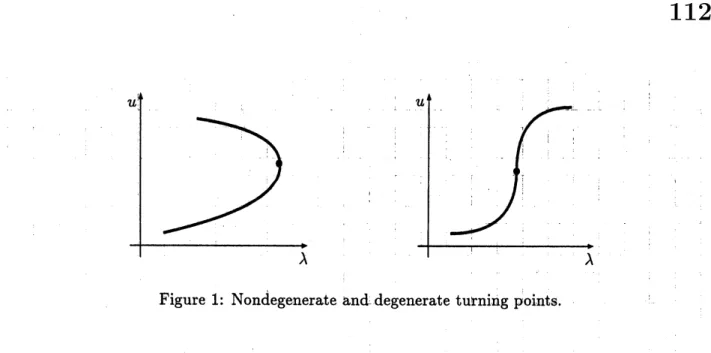
Figure 1: Nondegenerate and degenerate turning points.

where $\Omega\subset \mathbb{R}^{d}(d=1,2,3)$ is a bounded domain with the piecewise $C^{2}$ boundary $\partial\Omega$, and

$\tilde{\mathrm{a}}$ : $\Lambda\cross\overline{\Omega}\cross \mathbb{R}^{d1}+arrow \mathbb{R}^{d},$ _$f$ : $\Lambda\cross\overline{\Omega}\cross \mathbb{R}^{d+1}arrow \mathbb{R}$

are

sufficiently smooth $\mathrm{f}\mathrm{u}\mathrm{n}\mathrm{C}\mathrm{t}\mathrm{i}6\mathrm{n}\mathrm{s}$

.

Here, the

equation (1.1) is called strongly nonlinear if$\tilde{\mathrm{a}}(\lambda, x,y, z)(\lambda\in\Lambda, x\in\Omega, y\in \mathbb{R}, z\in \mathbb{R}^{d})$ is

nonlinear with respect to $z$

.

Otherwise, it is called mildly nonlinear.

Since the equation (1.1) is defined in $\mathrm{d}\mathrm{i}_{\mathrm{V}\mathrm{e}\mathrm{r}}\mathrm{g}\mathrm{e}|\mathrm{n}\mathrm{C}\mathrm{e}$ form, finite element

$\mathrm{s}\mathrm{o}\mathrm{l}\mathrm{u}\mathrm{t}\mathrm{l}\mathrm{o}\mathrm{n}\mathrm{s}|\prime \mathrm{t}.0|‘(1.1)$ is

defined in a natural way.

In [8], [9], and [13] Fink and $\dot{\mathrm{R}}$

heinboldt have shown that some subset of the solutions to

(1.1) form an one-dimensional smooth manifold without boundaries, if the $\mathrm{n}\mathrm{o}\mathrm{n}\mathrm{l}\mathrm{i}\overline{\mathrm{n}}\mathrm{e}\mathrm{a}\mathrm{r}$ operator

defined by (1.1) is Fr\’echet _{differentiable and Fredholm of index 1. They have also shown that}

corresponding finite element solutions forman one-dimensional smooth manifold. In this paper

we denote by $\mathcal{M}_{0}$ and $\mathcal{M}_{h}$ the exact solution manifold of (1.1) and the $\mathrm{C}\mathrm{o}\mathrm{r}\mathrm{r}\mathrm{e}\mathrm{s}\mathrm{P}^{\mathrm{o}}\mathrm{n}\mathrm{d}\mathrm{i}\mathrm{n}\dot{\mathrm{g}}$

. finite

element solution manifold, respectively.

Here, a linear operator $P\in \mathcal{L}(A, B)$ is called Fredholm if (1) the dimension of$\mathrm{K}\mathrm{e}\mathrm{r}P$ is

finite, (2) ${\rm Im} A\subset B$ is closed, (3) the dimension of $\mathrm{C}\mathrm{o}\mathrm{k}\mathrm{e}\mathrm{r}A:=B/{\rm Im} A$ is finite. If$P\in \mathcal{L}(A, B)$

is Fredholm, its index $\mathrm{i}\mathrm{n}\mathrm{d}P$ is defined by $\mathrm{i}\mathrm{n}\mathrm{d}P:=\dim \mathrm{K}\mathrm{e}\mathrm{r}P-\mathrm{d}_{1}^{\urcorner}\mathrm{m}\mathrm{c}_{\mathrm{o}\mathrm{k}}\mathrm{e}\mathrm{r}P$

.

Let _{$U\subset A$} be

open and $F:Uarrow B$ Fr\’echet _{differentiable.} $F$ is

cailed

Fredholm in $U$ ifits Fr\’echet derivative

$DF(u)\in \mathcal{L}(A, B)$ is Fredholm at any $u\in U$

.

It is shown that $\mathrm{i}\mathrm{n}\mathrm{d}DF(u)$ is constant in each

connected component of$U$

.

Hence, we define the index of$F$ by $\mathrm{i}\mathrm{n}\mathrm{d}F:=\mathrm{i}\mathrm{n}\mathrm{d}DF(u)$

.

In [17] and [18], it is shownthat, under$\mathrm{r}\mathrm{e}\mathrm{a}\mathrm{s}\mathrm{o}\mathrm{n}\mathrm{a}\mathrm{b}\mathrm{l}\underline{\mathrm{e}}$conditions, for each$\mathrm{c}\underline{\mathrm{o}\mathrm{m}}\mathrm{p}\mathrm{a}\mathrm{c}\mathrm{t}$subset

$\overline{\mathcal{M}}_{0}\subset$

$\lambda 4_{0}$, there exists a locally unique compact subset $\mathcal{M}_{h}\subset \mathcal{M}_{h}$ such that $\mathcal{M}_{0}$ is approximated

uniformly by $\mathcal{M}_{h}$, if triangulation of $\Omega$ is sufficiently fine.

$\mathrm{M}_{\mathrm{o}\mathrm{r}\mathrm{e}\mathrm{o}\mathrm{V}}\mathrm{e},\mathrm{r}$, several a priori error

estimates are obtained.

The aim of this paper is to refine the error analysis on branches around turning points.

A point $(\lambda, u)\in \mathcal{M}_{0}$ is called a turning point if the partial Fr\’echet derivative _{$D_{u}F(\lambda, u)\in$}

$\mathcal{L}(A, B)$ at $(\lambda, u)$ is not an isomorphism.

To develop a refined error analysis around a turning point, we introduce aslightly different

formulation of the problem from that in [17], and showa theorem which is similarto [18,

The-orem 8.6] and [17, Corollary 7.8]. Next, we obtain anelaborate error estimate of parameter. In

the following we explain the basic ideas of this paper.

In the error analysis of parametrized nonlinear equations, we have the following difficulty.

Suppose that we are approaching a turning point during continuation process of a solution

branch. Since we cannot fix the parameter $\lambda$ around a turning point in (1.1), $\lambda$ should be

treated as an unknown parameter. Hence, correspondence of an approximated solution to

an

Usually, this $\mathrm{d}\mathrm{i}\mathrm{f}\mathrm{f}\mathrm{i}_{\mathrm{C}\mathrm{u}}1\mathrm{t}\mathrm{y}$ is overcome by the following

mannet.

We introduce a (nonlinear, in

general) functional $\rho$: A $\cross Aarrow \mathbb{R}$, and consider the following problem—. (1.2) $H(\gamma, \lambda,u):=(\rho(\lambda, u)-\gamma,$$F(\lambda,u))=(0,\theta)^{-}\in \mathbb{R}\mathrm{x}A$,

where $H:\mathbb{R}\cross\Lambda\cross Aarrow \mathbb{R}\cross B$

.

We expect thatthe partialFr\’echet derivative$D_{(\lambda},{}_{u)}H(\gamma,$ $\lambda,$$u\mathrm{I}\in$

$\mathcal{L}(\mathbb{R}\cross A,\mathbb{R}\cross B)$ is an isomorphism at a turning point $(\lambda, u)$ and in its neighborhood. In

Section 2, it will be shown that, if$D_{\lambda}F(\lambda, u)\neq 0$ and $\mathrm{K}\mathrm{e}\mathrm{r}DF(\lambda,u)\mathrm{n}\mathrm{K}\mathrm{e}\mathrm{r}D\rho(\lambda,u)=\{(0,0)\}$

at $(\lambda, u)\in \mathcal{M}_{0}$, then the above partialFr\’echet derivative is an isomorphism. If$\mathrm{W}_{-}\mathrm{e}$ could find a

good definition of such $\rho$,

then

the solution branch would now be parametrizdd by $\gamma$

.

Finite element solutions $(\lambda_{h},u_{h})$ would be defined by :

(1.3) $H_{h}(\gamma, \lambda, u):=(\rho(\lambda h, uh)-\gamma,$$Fh(\lambda_{h},uh))=(0,0)$,

where $F_{h}$ is an approximation of$F$

.

In this setting the correspondence of an $\mathrm{e}\mathrm{x}\mathrm{a}\mathrm{c}\mathrm{t}|\mathrm{s}\mathrm{o}\mathrm{l}\mathrm{u}\mathrm{t}\mathrm{i}\mathrm{o}\mathrm{n}(\lambda, u)$

and an finite element solution $(\lambda_{h}, u_{h})$ is represented by $\rho(\lambda_{h}, u_{h})=\gamma=\rho(\lambda, u)$

.

In the above setting we will show that, even around a turning point, there exists a locally

unique finite element solution branch near an exact solution branch under suitable conditions.

Also, some error estimates of distance between the exact and finite element solution branches

are given.

Next, we will consider an elaborate error estimate ofparameter $\lambda$

.

In

error

analysis ofthe

finite element method (1.3) for (1.2) around a turning point,we would have

error

estimatessuch

as

$|\lambda-\lambda_{h}|+||u-u_{h}||_{A}\leq Ch^{r}$

.

In many practical computation, it is usually observed that the error $|\lambda-\lambda_{h}|$ is much smaller

than $||u-u_{h}||A$, or $Ch^{r}$

.

A typical and well-known example of this phenomenon is finite element approximation of

the eigenvalue problems:

(1.4) $-\triangle u=\lambda u$, $u\in H_{0}^{1}(\Omega)$

.

Let $(\lambda, u)$ be an eigen-pair of (1.4) and $(\lambda_{h}, u_{h})$ its finite element approximation. Suppose that

the eigenvalue $\lambda$ is simple. Then we have an error estimate such as

$|\lambda-\lambda_{h}|\leq C||u-u_{h}||_{H_{0}^{1}}^{2}$,

where $C$ is a positive constant independent of $h$ (see, for example, [14, Chapter 6], [1]).

We will show that a similar estimate hold for the finite element solutions $(\lambda_{h}, u_{h})$ of (1.3)

under the condition that $D_{u}F(\lambda,u)$ is seIf-adjoint. To obtain a similar estimate we introduce

an auxiliary equation. Let $z$ and $z_{h}$ be the exact and finite element solutions to the auxiliary

equation. We will show that the error $|\lambda-\lambda_{h}|$ is estimated as

$|\lambda-\lambda_{h}|\leq C||u-uh||_{A}(||u\sim-uh||_{A}+||z-Z_{h}||A)$

around a turning point, where $C$ is a positive constant independent of$h$

.

Occasionally, a turning point on the exact solution manifold $\mathcal{M}_{0}$ has a certain physical

meaning, and, in such a case, computing its precise value will become important. Ifa turning

associated finite

element

solution manifoldalso has a locally unique nondegenerate turning pDint

$(\lambda_{0’ 0}^{h}u^{h})\in \mathcal{M}_{h}$

.

The error $|\lambda_{0}-\lambda^{h}|0$ is estimated accurately by$|\mathrm{a}$-similar manRer $\mathrm{a}_{\mathrm{S}}$ abeve.

In Section 2 and 3 wedevelop ourtheory inan abstract $\mathrm{s}\mathrm{e}\mathrm{t}\mathrm{t}\mathrm{i}\mathrm{n}_{\mathrm{F}}.- \mathrm{A}_{\mathfrak{M}}1\mathrm{i}\mathrm{c}\mathrm{a}\mathrm{t}\mathrm{i}\mathrm{o}\mathrm{n}\mathrm{s}$ ofthe abstract

theoremsobtained in Section 2 and 3 to the strongly

nonlinear

elliptic $\mathrm{b}\mathrm{o}\mathrm{u}_{-}\mathrm{n}\mathrm{d}\mathrm{a}\mathrm{r}\mathrm{y}^{1}$value problem

(1.1) will be found in the original version ofthis paper.

2.

Abstract

Formulation.

In this section, we formulate our problem in an abstract setting, and show a theorem which

claims existence of a locally uniqu\’e solution branch of a discretized problem. The setting in this

section is slightly different from that of [17].

For the stage

of

our analysis $\mathrm{w}_{\mathrm{I}}\mathrm{e}$first introduce functional spaces.

(A1) There are Banach spaces, $V,$ $W$, and $X_{p}(1\leq p\leq\infty)$, where $X_{2}$ is a

$\dot{\mathrm{H}}$

ilbert space, such that $V\subset X_{\infty}\subset X_{p}(1\leq p\leq\infty)$ and $W\subset X_{1’}\subset X_{q}^{J}(1\leq q\leq\infty)$

.

Here, $X_{q}’$ is the dual

space of $X_{q}$

.

We suppose that all incIusions are continuous. We also suppose that $X_{r}$ is

dense in $X_{p}$ if $1\leq p\leq r<\infty$

.

Let $F$ : $\Lambda\cross X_{p}arrow X_{q}’(1/p+1/q=1)$ be a nonlinear map, where A $\subset \mathbb{R}$ is an interval.

We consider the parametrized nonlinear equation $F(\lambda, u)=0$

.

Since we will suppose that $F$ is

strongly nonlinear, the domain and the range should be taken carefully. In many cases, $F$ is not

Fr\’echet differentiable on $\Lambda\cross X_{p},$$p<\infty$, and should be restrictedto a certainsubspaceto make

it differentiable.

We also need extensions and restrictions of theFr\’echet derivatives $DF(\lambda, v),$ $DvF(\lambda, v)$ etc.

at $(\lambda, v)$

.

When we need to specify the domain of, say, $D_{v}F(\lambda,v)$ clearly, we will write such

as $D_{v}F(\lambda, v)\in \mathcal{L}(P, Q)$

.

This means that $D_{v}F(\lambda, v)$ now denotes its extension (or restriction)

whose domain is $P$ and range is in $Q$

.

Now, we take certain $p\geq 2$ and $q$ with $1/p+1/q=1$, and fix them. We then assume the

following:

(A2) The restriction of$F$ to $\Lambda\cross X_{\infty}$, denoted by $F$ again, is a Fr\’echet differentiable map from

$\Lambda\cross X_{\infty}$ to $X_{1}’$

.

For any $\lambda\in$ A and $v\in X_{\infty}$ the derivative $DF(\lambda, v)\in \mathcal{L}(\mathbb{R}\cross X_{\infty}, X_{1}’)$

can be extended to $DF(\lambda, v)\in \mathcal{L}(\mathbb{R}\cross X_{p}, X_{q}’)$ and it is locally Lipschitz continuous on

$\Lambda\cross X_{\infty}$: i.e., for any bounded convex set $\mathcal{O}\subset\Lambda\cross X_{\infty}$ there exists a positive constant $C_{1}(\mathcal{O})$ such that

$||DF(\lambda 1, v)-DF(\lambda 2, w)||_{c(,X_{q})}\mathbb{R}\mathrm{x}Xpl\leq C_{1}(\mathcal{O})(|\lambda_{1^{-}}\lambda 2|+||v-w||_{X_{\infty}})$

for arbitrary $(\lambda_{1}, v),$ $(\lambda_{2}, w)\in \mathcal{O}$

.

(A3) We suppose that thereexists an open subset $S\subset\Lambda\cross V$in which$F:Sarrow W$is a Fredholm

operator ofindex 1. We also suppose that, for each $(\lambda, u)\in S,$ $DF(\lambda, u)\in \mathcal{L}(\mathbb{R}\cross x_{p}, x_{q}’)$

is a Fredholm operator of index 1 as well.

We define the subset $R(F, S)\subset S$ by

$R(F, S):=$

{

$(\lambda,$$u)\in S|DF(\lambda,$$u)\in \mathcal{L}(\mathbb{R}\cross V,$$W)$ is

onto}.

The following lemma is valid:

(2) For $(\lambda,u)\in \mathcal{R}(F, S)$, we $h\mathrm{a}veeithe\overline{r}$ $|$

Case

1:

$\mathrm{K}\mathrm{e}\mathrm{r}D_{u}F(-\lambda, u)=\{0\}$ an$dE_{\lambda}F(\lambda,u)\in{\rm Im} R|F\{\lambda,u),-\partial \mathrm{r}$

’ Case2: $\mathrm{d}i\mathrm{m}\mathrm{K}\mathrm{e}\mathrm{r}\theta_{u}F\{\lambda,\mathrm{u}$) $=1$, and $D_{\lambda}F(\lambda, w)\not\in{\rm Im} D_{u}p\{\lambda,u$).

a

For the prodf, see [18, Section 4].

We introduce anonlinear functional $\rho$ : $\Lambda\cross|K_{p}arrow \mathbb{R}$and

assume

that

(A4) The restriction of$\rho$ to $\Lambda\cross X_{\infty}$, denoted by$\rho$ again, is Ff\’eche{differentiable. (A5)

$\mathrm{F}\mathrm{o}\mathrm{r}(\lambda \mathrm{e}\mathrm{X}\mathrm{t}\mathrm{e}\mathrm{n}\mathrm{d}’\epsilon u\mathrm{d})\in\Lambda X_{\infty},$$\mathrm{t}\mathrm{h}\mathrm{e}\mathrm{F}\mathrm{r}\acute{\mathrm{e}}\mathrm{C}\mathrm{h}\mathrm{e}\mathrm{t}\mathrm{d}\mathrm{e}\mathrm{r}\mathrm{i}\mathrm{t}\mathrm{o}D^{\cross}\rho(\lambda,u)\in \mathcal{L}(\mathbb{R}\cross x\mathbb{R})p’(=\mathbb{R}\ltimes x^{\rho(\lambda,u)(\mathbb{R}}/)p’ \mathrm{y}’ \mathrm{i}\mathrm{v}\mathrm{a}\mathrm{t}\mathrm{i}\mathrm{V}\acute{\mathrm{e}}D\mathrm{a}\mathrm{n}\mathrm{d}\mathrm{i}\in \mathrm{t}\mathrm{i}\mathrm{s}!c.\mathrm{o}_{-\mathrm{C}\mathrm{a}1}\mathrm{x}X_{\infty}1\mathrm{L}\mathbb{R}\mathrm{b})(=\mathbb{R}\mathrm{S}\mathrm{C}\mathrm{h}\mathrm{i}\mathrm{t}\mathrm{Z}\rfloor_{\mathrm{C}}^{\mathrm{X}x_{\infty}’)}\mathrm{o}\mathrm{n}\mathrm{t}\mathrm{i}\mathrm{n}\mathrm{u}\mathrm{c}\mathrm{a}\mathrm{o}\mathrm{u}\mathrm{s}\mathrm{n}_{\mathrm{o}\mathrm{n}}\mathrm{b}\mathrm{e}$

$\Lambda\cross X_{\infty}$, i.e., for any bounded convexset $\mathcal{O}\subset\Lambda\cross X_{\infty}$, there exists a positive constant $C_{2}(\mathcal{O})$ such that

$||D\rho(\lambda 1,v)-D\rho(\lambda_{2}, w)||_{\mathbb{R}}\cross X’\mathrm{p}\leq c_{2}(\dot{\mathcal{O}})(:|\lambda_{1}-\lambda_{2}|+||v-w||x\infty)$

for any $(\lambda_{1}, v),$ $(\lambda_{2}, w)\in$ O.

(A6) Let $(\lambda, u)\in S$ and _{$D_{u}F(\lambda, u)\in \mathcal{L}(X_{p},X’.)q$}

.

We suppose $\mathrm{t}\mathrm{h}\mathrm{a}\mathrm{t}\backslash$

. if $D_{u}F(\lambda,u)\psi=f$ for

$\psi\in X_{p}$ and $f\in W$, then $\psi\in V$

.

Lemma 2.2. $Ass\mathrm{u}me$ that $(A1)-(A6)$ are valid. Suppos$e$ that there is $(\lambda 0, u_{0})\in R(F, S)$

such that $D_{\lambda}F(\lambda_{0}, u_{0})\neq 0\in$ W. From $(A3)$, there exists $(\mu_{0}, \psi 0)\in \mathbb{R}\cross V$ such that

$\mathrm{K}\mathrm{e}\mathrm{r}DF(\lambda_{0}, u\mathrm{o})=\mathrm{s}\mathrm{p}\mathrm{a}\mathrm{n}\{(\mu_{0},\psi_{0})\}$

.

We $\mathrm{a}ss\mathrm{u}\mathrm{m}e$ that$D\rho(\lambda 0, u_{0})(\mu 0, \psi 0)\neq 0\in \mathbb{R}$

.

$\mathrm{t}$

Define $G:\Lambda\cross Warrow \mathbb{R}\cross V$ by$G(\lambda, u):=(\rho(\lambda, u)-\gamma,$$F(\lambda, u))$

,

where$\gamma\in \mathbb{R}$

.

Then, $DG(\lambda_{0}, u\mathrm{o})\in \mathcal{L}(\mathbb{R}\cross W, \mathbb{R}\cross V)$ is an

iso‘m

orphism. Moreover, $DG_{1}(\lambda 0, u\mathrm{o})\in \mathcal{L}(\mathbb{R}\cross$

$X_{p},$$\mathbb{R}\cross X_{q}’)$ isan isomorphism as well.

Proof.

From the assumptions we find that $\mathrm{K}\mathrm{e}\mathrm{r}DF(\lambda_{0}, u\mathrm{o})\cap \mathrm{K}\mathrm{e}\mathrm{r}D\rho(\lambda 0,u\mathrm{o})=\{(0,0)\}$

.

This

implies that $\mathrm{K}\mathrm{e}\mathrm{r}DG(\lambda_{00)},$$u$ is trivial and $DG(\lambda_{0}, u_{0})$ is $\mathrm{o}\mathrm{n}\mathrm{e}-\mathrm{t}_{0- \mathrm{o}\mathrm{n}\mathrm{e}}$

.

Since$DF(\lambda_{0}, u_{0})$ is onto, for any$g\in W$

,

there is$(\nu, \varphi)\in \mathbb{R}\cross V$ suchthat$DF(\lambda 0, u\mathrm{o})(\nu, \varphi)=$

$g$

.

Since $D\rho(\lambda_{0}, u_{0})(\mu 0,\psi 0)\neq 0$, for any $t\in \mathbb{R}$ there is

$\alpha\in \mathrm{R}$ such that $D\rho(\lambda_{0}, u\mathrm{o})((\nu, \varphi)+$

$\alpha(\mu_{0},$$\psi_{0))}=t$

.

This yields that $DG(\lambda 0, u_{0})$ is onto. Therefore, $DG(\lambda 0, u\mathrm{o})\in \mathcal{L}(\mathbb{R}\mathrm{x}V, \mathbb{R}\cross W)$

is an isomorphism.

To show that $DG(\lambda_{0}, u\mathrm{o})\in L(\mathbb{R}\cross X_{p}, \mathbb{R}\cross X_{q}’)$ is an $\mathrm{i}_{\mathrm{S}\mathrm{o}\mathrm{m}\mathrm{o}}\mathrm{r}\mathrm{p}\mathrm{h}\dot{\mathrm{B}}\mathrm{m}$

,

we first show that

$DF(\lambda 0, u\mathrm{o})\in \mathcal{L}(\mathbb{R}\cross X_{p}, X_{q}’)$ is onto. Since $DF(\lambda_{0}, u\mathrm{o})\in \mathcal{L}(\mathbb{R}\cross X_{p}, X_{q}’)$ isFredholm with index

1 by (A3), we only have to show that the dimension of$\mathrm{K}\mathrm{e}\mathrm{r}DF(\lambda 0, u\mathrm{o})\subset \mathbb{R}\cross X_{p}$ is 1.

Let $(\mu, \psi)\in \mathbb{R}\cross X_{p}$ be such that $DF(\lambda_{0}, u_{0})(\mu, \psi)=0\in X_{q}’$

.

This is also written as $D_{u}F(\lambda_{0}, u\mathrm{o})\psi=-\mu D_{\lambda}F(\lambda_{0}, u\mathrm{o})$

.

Since $D_{\lambda}F(\lambda_{0},u\mathrm{o})\in W$ and (A6), we conclude that $\psi\in W$

and $\dim \mathrm{K}\mathrm{e}\mathrm{r}(DF(\lambda 0, u\mathrm{o})\in \mathcal{L}(\mathbb{R}\cross XX_{q}p’/))=1$

.

Using this fact, we show that $DG(\lambda 0, u\mathrm{o})\in \mathcal{L}(\mathbb{R}\cross X_{p}, \mathbb{R}\cross X_{q}’)$ is an isomorphism by the

exactly same manner as above. $\square$

Corollary 2.3. Assume that $(A1)-(A6)$ are vali$d$

.

Suppose that th$ere$ exists $(\lambda_{0}, u_{0})\in$

$\mathcal{R}(F, S)$ such that $F(\lambda_{0}, u_{0})=0,$ $\rho(\lambda_{0}, u_{0})=\gamma_{0}$, and $D_{\lambda}F(\lambda_{0}, u\mathrm{o})j|\neq 0$

.

Suppose also that $\mathrm{K}\mathrm{e}\mathrm{r}DF(\lambda 0, u\mathrm{o})\cap \mathrm{K}\mathrm{e}\mathrm{r}D\rho(\lambda 0, u\mathrm{o})=\{(0,0)\}$

.

Define $H$

:

$\mathbb{R}\cross\Lambda\cross Varrow \mathbb{R}\mathrm{x}W$ by$H(\gamma, \lambda, u)$ $:=$

$(\rho(\lambda, u)-\gamma,$$F(\lambda, u\mathrm{I})$

.

Then, we have $H(\gamma_{0}, \lambda_{0},u_{0})=(0,0)$ an$\mathrm{d}D_{(\lambda},{}_{u)}H(\gamma 0, \lambda 0, u_{0})\in \mathcal{L}(\mathbb{R}\cross V, \mathbb{R}\cross W)$ is an

isomorphism. Therefore, by the implicit function theorem, there exist apositive constant $\epsilon$ and

a $C^{1}$ map $(\gamma_{0^{-\epsilon}}, \gamma 0+\epsilon)\ni\gamma-\rangle(\lambda(\gamma),u(\gamma))\in\Lambda\cross V$ such that $(\lambda(\gamma_{0}),u(\gamma_{0}))=(\lambda_{0}, u\mathrm{o})$ and $H(\gamma, \lambda(\gamma),$$u(\gamma))=(0,0)$ for any $\gamma$

.

That is, the

$sol\mathrm{u}$tion _$m$anifold of the $eq\mathrm{u}a$tion $F(\lambda, u)=0$

To define $\mathrm{d}\mathrm{i}_{9\mathrm{C}}\mathrm{r}\mathrm{e}\mathrm{t}\mathrm{i}\mathrm{z}\mathrm{e}\mathrm{d}$ solutions of$F(\lambda, u)=0$, we introduce thefinite-dimensipnal

subspaces

$S_{h}\subset X_{\infty}$ which are parametriaed by $h,$ $0<h<1$ with the$\mathrm{f}\mathrm{o}\mathrm{f}\mathrm{l}\mathrm{o}\mathrm{W}\dot{\mathrm{k}}\mathrm{n}\mathrm{g}$ properties:

(A7) There exists a real $r\geq 0$ and apositive

constant

$C_{3}$ independent of$h$ suuch that

$||v_{h}|| \mathrm{x}\infty\leq\frac{C_{3}}{h^{r}}||v_{h}||\mathrm{x}p$

’ $\forall v_{h}\in S_{h}$

.

The relations of Banach spaces are depicted in the following:

AX$s_{h}$

$\cap$

$\Lambda\cross V$ $\subset$ $\Lambda\cross X_{\infty}$ $\subset$ $\mathbb{R}\cross X_{p}$ $\subset$ $\mathbb{R}\cross X_{2}$ $\downarrow F(\lambda, u)$ $\downarrow F(\lambda, u)$ $\downarrow DF(\lambda,u)$ $\downarrow DF(\lambda,u)$ $W$ $\subset$ $X_{1}^{/}$ $\subset$ $X_{q}’$ $\subset$ $X_{2}^{/}$

The finite element solution $(\lambda_{h}, u_{h})\in\Lambda\cross S_{h}$is defined naturally by

$\langle F(\lambda_{h}, u_{h}), v_{h}\rangle=0$, $\forall v_{h}\in S_{h}$,

where $\langle\cdot, \cdot\rangle$ is the duality pair of$X_{2}^{\prime^{\iota}}$and $X_{2}$

.

We derive an equivalent definition of the finite

element solutions which is more convenient in the error analysis.

Let $Q\in \mathcal{L}(X_{2}, x_{2}’)$ be a self-adjoint operator, that is, $\langle Qu, v\rangle=\langle Qv, u\rangle$ for all _$u,$$v\in X_{2}$

.

Suppose that there exists a positive constant $\alpha$ such that

(2.1) $(Qv,$$v\rangle\geq\alpha||v||_{\mathrm{x}}^{2}2’$ $\forall v\in X_{2}$

.

We define $(\cdot, \cdot)_{Q}$ by $(u,v)_{Q}:=\langle Qu, v\rangle$

.

It is easy to show that $(\cdot, \cdot)_{Q}$ is an inner product and

the norm $||v||_{Q}:=(v, v)_{Q}^{1/2}$ is equivalent to the original norm $||v||x_{2}$

.

It is also easyto showthat

$Q\in \mathcal{L}(X_{2}, x_{2}/)$ is an isomorphism.

We define the canonical projection$\tilde{P}_{h}$ :

$X_{2}arrow S_{h}$ by $(\psi_{-\tilde{P}_{h}}\psi, vh)_{Q}=0$for all$v_{h}\in S_{h}$

.

Ob-viously, we have that $(u,\tilde{P}_{h}v)_{Q}=(\tilde{P}_{h}u, v)_{Q}$for all_$u,$$v\in X_{2}$

.

Asin [18, Section 6] it follows from

the definitions that $(\lambda_{h}, u_{h})$ is a finite element solution if and only if $(Q\tilde{P}_{hQ^{-1}}F(\lambda h, u_{h}),$ $v)=0$

for all $v\in X_{2}$

.

Following Fink and Rheinboldt ([8], [9], [13]) we define the approximation of$F(\lambda, u)$ by

(2.2) $F_{h}(\lambda, u):=(I-P_{h})Qu+P_{h}F(\lambda, u)$

,

$P_{h}:=Q\tilde{P}_{h}Q^{-1}$

,

where $I$ is the identity of$X_{2}’$

.

It can be seen easily [13, Lemma 5.1] that $F_{h}(\lambda, u)=0$ if and

only if$u\in S_{h}$ and $(\lambda, u)$ is a finite element solution.

Theorem 2.4. $Ass\mathrm{u}m\mathrm{e}$ that $(A1)-(A7)$

are

valid. Suppose that th_$ere$ exists $(\lambda 0, u\mathrm{o})\in$

$\mathcal{R}(F, S)$ such that $F(\lambda 0, u\mathrm{o})=0,$ $\rho(\lambda_{0}, u_{0})=\gamma_{0}$, and $D_{\lambda}F(\lambda 0, u\mathrm{o})\neq 0$

.

Suppose also that

$\mathrm{K}\mathrm{e}\mathrm{r}DF(\lambda 0, u\mathrm{o})\mathrm{n}\mathrm{K}\mathrm{e}\mathrm{r}D\rho(\lambda 0, u\mathrm{o})=\{(0,0)\}$

.

Then, by Corollary 2.3, thereexist a positiveconstant $\epsilon_{0}$ anda

$C^{1}$ map _{$[\gamma 0-\epsilon 0, \gamma 0+\epsilon_{0}]\ni\gamma\mapsto(\lambda(\gamma), u(\gamma))\in\Lambda\cross V$} such that _{$(\lambda(\gamma_{0}), u(\gamma 0))=(\lambda_{0}, u_{0})$},

$\gamma=\rho(\lambda(\gamma), u(\gamma))$, and $F(\lambda(\gamma), u(\gamma))=0$

.

We assume that $(\lambda(\gamma), u(\gamma))\in \mathcal{R}(F, S)$ for all

$\gamma\in[\gamma_{0^{-}6}0, \gamma 0+\epsilon_{0}]$

.

We also assume that there exists the projection II$h$

:

$X_{p}arrow S_{h}$ for each

$h>0$ such that, forall $\gamma\in[\gamma_{0}-\epsilon 0, \gamma_{0}+\epsilon_{0}]$,

(2.3) $\lim_{harrow 0}h^{-r}||u(\gamma)-\Pi hu(\gamma)||_{X_{\mathrm{p}}}=0$,

and the above convergences $a\mathrm{r}\rho$ uniform.

$We$, on the other hand,

suppose

that$B_{u}F$($\lambda\sigma,u\mathrm{o}+is$ deeoznposedinte$\partial_{\overline{u}}P\{*,\# 0$) _{$=- Q+$}

$R$, where $Q\in \mathcal{L}(X_{p}, \ovalbox{\tt\small REJECT}_{q})$ is the principal

$par\mathrm{t}_{\overline{|}}$-whicA-is

$seff\neg ad^{s}j\mathrm{o}i\overline{n}i$

and

satiffies (2.1), and

$R\in \mathcal{L}(X_{\mathrm{P}’ q}X/)$ is compact. Thhe discretized nolllinear map$F_{h}$ : $X_{p}arrow X_{q}’\mathrm{a}_{-}nd|_{the_{P^{r}}}ojection$ $P_{h}$ :$X_{q}’arrow X_{q}’i5d$efi$\mathrm{n}ed$ by (2.2). We

suppose tbat

(2.5) $h1\mathrm{i}^{1}\mathrm{m}arrow 0^{1\dagger}\psi-P_{h}\psi||_{X_{q}’}=\Theta$, $\forall\psi\in X_{q}/$

.

Then, for sufficien$tly$ small $h>0$, there exist

a-

positive $conStantI\epsilon_{1}\leq\epsilon_{0}|a\mathrm{n}d$

a-

uniq

$\mathrm{u}e_{}$

map $[\gamma 0-\epsilon 1,\gamma 0+\epsilon_{1}]\ni\gamma\mapsto(\lambda_{h}(\gamma),u_{h(\gamma)})\in\Lambda\cross S_{h}$ such

$tf_{\mathit{1}a},.\mathrm{t}Fh(\lambda h(\gamma),u_{h(}’|\gamma))=0\backslash for$

$\mathrm{a}ll$

,

$\gamma\in[\gamma_{0}-\in_{1}, \gamma_{0}+\epsilon_{1}]$

.

Moreover, we have the estimate

$|\lambda(\gamma)-\lambda_{h}(\gamma)|+\mathrm{H}u_{h(}\gamma)-\Pi_{h}u(\gamma)||\mathrm{x}_{p}\leq K_{1}||u(\gamma)-\Pi hu(\gamma)||X_{p}$

,

for all$\gamma\in[\gamma 0-\epsilon 1, \gamma 0+\epsilon_{1}]$, vvhere $K_{1}$ is a positive constant independen$t$ of$h$ and

$\gamma$

.

Proof.

The proof of Theorem 2.4 is quite

similar

to those of [$l7$

,

Theorem 7.7] and [18,

Theo-rem 8.4]. Hence, we here skip the proof. $\square$

3.

Elaborate Error

Estimates

of the Pararmeter

$\lambda$

.

In this section we give elaborate error estimates of the parameter $\lambda$

.

To do this we need more

assumptions.

(A8) The nonlinear maps $F:\Lambda\cross X_{\infty}arrow X_{1}’$ and $\rho:\Lambda\cross X_{\infty}arrow \mathbb{R}$are of$C^{2}\mathrm{c}$

las.s.

(A9) For any $(\lambda, u)\in S\subset\Lambda\cross W,$ $D_{u}F(\lambda, u)\in \mathcal{L}(X_{2}, x_{2}/)$ is self-adjoint.

Now, let $(\lambda, u)\in \mathcal{R}(F, S)$ be a solution of$F(\lambda_{\gamma}u)=0$ at which all assumptions of

Theo-rem 2.4 and (A8), (A9) hold. Let $(\lambda_{h}, u_{h})\in\Lambda\cross S_{h}$ be the corresponding finite element solution

with $\rho(\lambda_{h}, u_{h})=\rho(\lambda, u)$

.

We consider the following auxiliary problem: find $(\eta, z)\in \mathbb{R}\cross X_{p}$ such that

$\langle(D_{u}F^{0})_{Z}, v\rangle=\eta\{D_{u}\rho^{0},v\rangle$, $\forall v\in X_{p}$,

(3.1)

$(D_{\lambda}F0,$$z\rangle-\eta D_{\lambda}\rho 0=1$,

where $D_{u}F^{0}:=D_{u}F(\lambda,u),$ $D_{u}\rho^{0}:=D_{u}\rho(\lambda, u)$, etc.

Lemma 3.1. Suppose that all$ass$umptions of Theorem 2.4 and $(A8),$ $(A9)hol\mathrm{d}$

.

Then, the

$eq$uation (3.1) $h$as an uniq_$ue$solution $(\eta, z)\in \mathbb{R}\cross X_{p}$

.

Proof.

Recall that we have either

Case 1: $\mathrm{K}\mathrm{e}\mathrm{r}D_{u}F(\lambda,u)=\{0\}$ and $D_{\lambda}F(\lambda, u)\in{\rm Im} D_{u}F(\lambda,u)$, or

Case 2: $\dim \mathrm{K}\mathrm{e}\mathrm{r}D_{u}F(\lambda, u)=1$, and $D_{\lambda}F(\lambda, u)\not\in{\rm Im} D_{u}F(\lambda, u)$

.

Suppose that we are in Case 1. Then, $\mathrm{K}\mathrm{e}\mathrm{r}DF(\lambda, u)=\mathrm{s}\mathrm{p}\mathrm{a}\mathrm{n}\mathrm{t}(1, -(D_{u}F0)-1(D_{\lambda}F0))\}$

.

By

the assumption we have $D\rho^{0}(1, -(D_{u}F^{0})^{-1}(D_{\lambda}F0))$

. $\neq 0$, that is,

$D_{\lambda\rho^{0}-}\langle D_{u}\rho^{0}, (D_{u}F^{0})-1(D_{\lambda}p^{0})\rangle\neq 0$

.

Let $\eta:=(\langle D_{u}\rho^{0}, (D_{u}F^{0})-1(D_{\lambda}F0)\rangle-D\lambda\rho^{0})-1$ and $z:=\eta(D_{u}F^{0})-1(D_{u\beta}0)$

.

Since $D_{u}F^{0}$ is

self-adjoint by (A9), we have

and $\langle D_{\lambda}F^{0}, \ovalbox{\tt\small REJECT}\rangle-\eta D_{\lambda\rho^{0}}’=\eta(\langle D_{\mathrm{u}^{\rho^{0}}}, (D_{u}F^{01})^{-}(D\lambda F\mathrm{U})\rangle-D_{\lambda}p^{0}),=|\backslash 1$

.

$\mathrm{H}\mathrm{e}\mathrm{n}\mathrm{c}\mathrm{e}:(\eta,’ z’.)1-\mathrm{S}$a $\mathrm{s}\mathrm{o}\mathrm{l}\mathrm{l},1\mathrm{t}\mathrm{I}\tau$

.ion

of

(3.1). Uniqueness is $\mathrm{P}^{\mathrm{r}\mathrm{o}\mathrm{V}}\mathrm{e}A$-by thesame manner.

Now, suppose that we have Case 2. Then, there-exists $\dot{\psi}_{0}\in V$

such that $\mathrm{K}^{-}\mathrm{e}\mathrm{r}D:F(\lambda, \mathfrak{U})=$ $\mathrm{s}\mathrm{p}\mathrm{a}\mathrm{n}\{(0, \psi 0)\}$ and $\langle D_{u}\rho^{0}, \psi 0\rangle\neq 0$

.

Since $DF(\lambda,u_{})$ is onto, there exists $(\theta, \phi)\vee\in \mathbb{R}\cross X_{p}$such

that

. $\cdot$

’

.

1

(3.2) $\theta\langle D_{\lambda}F0, v\rangle+\langle(D_{u}F^{0})\phi, v\rangle=\mathrm{f}^{D_{u}\rangle}\rho^{0},$$\prime \mathrm{i}f$ , $\forall’\theta\in X_{2}$,

and $\theta$ is determined uniquely.

We claim that $D_{u}\rho^{0}\not\in{\rm Im}(D_{u}F0)$

.

If $D_{u}\rho^{0}\in{\rm Im}(D_{u}F^{0})$, then there $\mathrm{w}\mathrm{o}\mathrm{u}\Gamma \mathrm{d}$ exist _{$w\in X_{p}$}

such that $(D_{u}F^{0})w=D_{u}\rho^{0}$

.

Hence, we have

$0\neq\langle D_{u}\rho^{0},$$\psi_{0})=\langle(D_{u}F^{0})w,$ $\psi_{0}\}=\langle(D_{u}F0)\psi 0,w\rangle=0$,

and obtain a $\mathrm{C}\mathrm{o}\mathrm{n}\mathrm{t}\mathrm{r}\mathrm{a}\mathrm{d}\mathrm{i}\mathrm{c}\mathrm{t}\mathrm{l}\mathrm{o}\mathrm{n}*$

.

Therefore, we conclude that $D_{u}p^{0}\not\in{\rm Im}(D_{u}F^{0})$ and $\theta\neq 0$

.

Letting $v:=\psi_{0}$ in (3.2), we have $\theta\langle D-\lambda F^{0},$$\psi_{0\rangle}=(D_{u}\rho^{0},$ $\psi_{0\rangle}\neq 0.$ $\mathrm{H}\mathrm{e}_{\mathrm{I}}\mathrm{n}\mathrm{c}\mathrm{e}_{!}$, we conclude

($D_{\lambda}F^{0},$ $\psi 0\rangle=\langle$ $D_{u}\rho^{0},$ $\psi_{0\rangle}/\theta\neq 0$

.

We thus immediatelynoticethat $(0,$$\alpha\psi 0)$with$\alpha:=(D_{\lambda}F^{0},$$\psi_{0}\rangle$$-1$

is a solution of (3.1). Again, the uniqueness is shown by the

same manner.

$\square$

It is obvious that we may apply Theorem 2.4 totheequation (3.1) with the $\mathrm{f}\mathrm{o}1\dot{1}$

owing$\dot{\mathrm{s}}$

etting:

$F(\eta, z):=(D_{u}F0)z-\eta(Du\rho 0)$

,

$\rho(\eta, z):=\langle D\lambda F^{0},$ $z)-\eta(D_{\lambda}\rho^{0})$,

and obtain

Lemma 3.2. For sufficiently $sm$all $h>0$, there exists th$\mathrm{e}$ unique finite element solution

$(\eta h, zh)\in \mathbb{R}\cross S_{h}$ of(3.1) such that

$\langle(D_{u}F^{0})_{Z_{h}}, vh\rangle=\eta_{h}(Du\rho^{0},$$vh\rangle,$ $\forall v\in S_{h}$, $\langle D_{\lambda}F^{00}, z_{h}\rangle-\eta hD_{\lambda}\rho=1$

.

Moreover, we have the estimate

$|\eta-\eta h|+||z-Zh||x_{p}\leq C||Z-\Pi_{h^{Z}}||X_{\mathrm{p}}$,

where $C$ is a positi$\mathrm{r}^{r}e$ constant independent of$h$

.

$\square$

Let $(\lambda, u)\in R(F, S)$ is a solution of $F(\lambda, u)=0$ which satisfies the assumptions of

Theo-rem 2.4 and (A8), (A9), and $(\lambda_{h}, u_{h})\in\Lambda\cross S_{h}$ the corresponding finite element solution. By

Taylor’s theorem and $\langle F(\lambda_{h}, u_{h}), vh\rangle=\langle F(\lambda, u), vh\rangle=0$ for any $v_{h}\in S_{h}$, we have

$0=( \lambda_{h}-\lambda)\langle D\lambda F^{00}, v_{h}\rangle+((DuF)(u_{h}-u), vh\rangle+\frac{1}{2}(\lambda_{h}-\lambda)^{2}(D\lambda\lambda F^{0},$$vh\rangle$

(3.3)

$+( \lambda_{h}-\lambda)\langle(D_{\lambda u}F^{0})(u_{h}-u), vh\rangle+\frac{1}{2}\langle(D_{uu}F^{0})(uh-u)^{2},v_{h}\rangle$,

where

$D_{\lambda\lambda}F^{0}:= \int_{0}^{1}(1-s)D\lambda\lambda F(\lambda+s(\lambda_{h}-\lambda), u+s(uh-u))d_{S}$,

$(D_{\lambda u}F^{0})(u_{h}-u):= \int_{0}^{1}(1-S)D\lambda uF(\lambda+S(\lambda h-\lambda), u+s(uh-u))(uh-u)d_{\mathit{8}}$,

Letting $v$ $:=$ . $u-u_{h}$ in (3.1), we $0.\mathfrak{b}$taln $-.\cdot$ . $\iota$ : $-$

$((D_{u}F^{0})_{Z}.’ u-uh\rangle=\langle(\dot{D}_{u}F0)(u_{1}-‘ uh),Z^{\backslash })..=\eta.\langle D_{\mathrm{a}}p,\dot{u}-0.u_{h}$)

$.\cdot$ Since $0=\rho(\lambda h,u_{h})-\rho(\lambda,u.)$ . $\cdot$ ..$\cdot$ .

$=( \lambda_{h}-\lambda)(D_{\lambda p}0)+\langle D_{u}\rho 0,-hu.\rangle u+\frac{1}{2}(\lambda_{\hslash}-\lambda)2(\acute{D}\lambda\lambda.\rho^{0})$

$+( \lambda_{h}-\lambda)(D_{\lambda}u\rho)0(u_{h}-u)+.\frac{1}{2}.(Duu\rho 0)(u_{h}arrow u)^{2}$

,

where

$D_{\lambda\lambda\rho^{0}}:= \int_{0}^{1}(1-s)D\lambda\lambda\rho(\lambda+s(\lambda_{h}-\lambda), u+4u_{h^{-}}u))ds$,

$(D_{\lambda u}\rho^{0})(uh-u)$ $:= \int_{0}^{1}(1-s)\langle D_{\lambda\rho(\lambda}u+s(\lambda_{h}-\lambda),u+s(u_{h}-u)), uh-w\rangle ds$,

$(D_{uu} \rho)0(uh-u)2:=\int_{0}^{1}(1-s)\langle D_{uu}\rho(\lambda+s(\lambda_{h}-\lambda), u+s(u_{h}-u))(u_{h}-u), u_{h}-u\rangle dS$,

we

have

$\langle(D_{u}F^{0})(u-u_{h}), Z\rangle=-\eta(\lambda-\lambda h)(D\lambda\rho^{0})+\frac{\eta}{2}(\lambda_{h}-\lambda)^{2}(Dk\lambda\rho)0$ (3.4)

$+ \eta(\lambda_{h^{-}}\lambda)(D_{\lambda\rho^{0}}u)(u_{h}-u)+\frac{\eta}{2}|(D_{uu}\rho^{02})(u_{h}-u)$

.

It follows from (3.3) with$v_{h}:=z_{h}$ (recall that $(\eta_{h}, z_{h})\in \mathbb{R}\cross S_{h}$

. isthe finite element solution

of (3.1)$)$ and (3.4) that

$(\lambda-\lambda_{h})(\langle D_{\lambda}F^{0}, z\rangle-\eta(D_{\lambda\rho^{0}})+B_{h})=\langle(D_{u}F^{0})(u-u_{h}), z-z_{h}\rangle$

$+ \frac{1}{2}\langle(D_{uu}F0)(u-u_{h})^{2}, z_{h}\rangle-\frac{\eta}{2}(Duu\rho^{02})(u-u_{h})$,

where $\lim_{harrow 0B_{h}}=0$

.

Therefore, we have proved the following theorem:

Theorem 3.3. Let $(\lambda, u)\in \mathcal{R}(F, S)$ be a solution of$F(\lambda, u)=0$ which satisfies the

as-sumptions of Theorem 2.4 and $(A8),$ $(A9)$

.

Let $(\lambda_{h}, u_{h})\in\Lambda\cross S_{h}$ be the corresponding finite

element solution. Let $(\eta, z)\in \mathbb{R}\cross X_{p}$ and $(\eta_{h}, z_{h})\in \mathbb{R}\cross S_{h}$ be the exact an$d$ the finite element

solutions $of(3.1)$

.

Then, for sufficiently small $h>0$

,

we have the following$ela$borate error estimate$of|\lambda-\lambda_{h}|$:

$| \lambda-\lambda_{h}|\leq C_{h}|\langle(D_{u}F^{0})(u-uh), z-zh\rangle+\frac{1}{2}\langle(D_{uu}F^{0})(u-u_{h})^{2}, zh\rangle$

$- \frac{\eta}{2}(D_{uu}\rho^{021})(u-u_{h})$,

where $D_{u}F^{0}:=D_{u}F(\lambda, u)$,

$(D_{uu}F^{02})(u-u_{h}):= \int_{0}^{1}(1-s)D_{u}uF(\lambda+s(\lambda_{h}-\lambda), u+s(u_{h}-u))(u-u_{h})^{2}d_{S}$,

$(D_{uu} \rho)0(u-u_{h})2:=\int_{0}^{1}(1-s)(D_{uu}\rho(\lambda+s(\lambda_{h}-\lambda), u+s(u_{h}-u))(u-u_{h}),$$u-uh\rangle ds$

,

equatim $F(\lambda, u)=0$ at $\mathrm{W}\mathrm{h}\mathrm{i}_{\mathrm{C}}\mathrm{h}^{- \mathrm{t}\mathrm{h}\mathrm{t}}\mathrm{e}^{-}\mathrm{a}\mathrm{S}\mathrm{s}\mathrm{u}m\mathrm{p}\dot{\mathrm{r}}\mathrm{o}\mathrm{n}\mathrm{S}$of $\mathrm{T}\mathrm{h}\mathrm{e}\mathrm{o}\mathrm{r}\mathrm{e}\mathrm{m}-- 2-.4^{-}\mathrm{B}\mathrm{n}\mathrm{d}$ (A8),

$|(A9)$ hold. That

is, $F(\lambda_{0}, u\mathrm{o})=0,$ $DF(|\lambda 0, u\mathrm{o})\in \mathcal{L}$($\mathbb{R}\cross V,$W-) is onto,

and

$D_{-w}|F_{-}(.\lambda. 0, u\mathrm{o})\in \mathcal{L}(V, W)$

$\mathrm{i}\mathrm{s}\mathrm{n}\mathrm{o}\mathrm{t}\uparrow$

an.

$\mathrm{I}\mathrm{t}\mathrm{t}\mathrm{h}\mathrm{e}\mathrm{I}\mathrm{i}\mathrm{S}\mathrm{o}\mathrm{m}\mathrm{o}\iota \mathrm{p}\mathrm{A}\mathrm{i}\mathrm{s}_{1}\mathrm{m}.\mathrm{I}\mathrm{n}\mathrm{t}\mathrm{h}\mathrm{i}\mathrm{S}\mathrm{c}\mathrm{a}\mathrm{S}\mathrm{e}\mathrm{W}\mathrm{e}\mathrm{h}\mathrm{a}_{\mathrm{f}}\mathrm{v}_{\mathrm{L}}\mathrm{e}\mathrm{d}\mathrm{i}\mathrm{m}\mathrm{K}\mathrm{e}_{3}\mathrm{r}DuF(\lambda\theta, \mu 0)=1\mathrm{a}\mathrm{n}\mathrm{d}D_{\star^{F}}1\mathrm{f}\mathrm{o}1\mathrm{o}\mathrm{w}\mathrm{s}\mathrm{f}\mathrm{r}\mathrm{o}\mathrm{m}\mathrm{t}\mathrm{h}\mathrm{e}\mathrm{p}\mathrm{r}o\mathrm{o}\mathrm{f}\mathrm{o}\mathrm{e}\mathrm{m}\mathrm{m}\mathrm{a}.1\mathrm{t}\mathrm{h}\mathrm{a}\mathrm{t}(3^{1}|1)\mathrm{h}\mathrm{a}\mathrm{S}\mathrm{a}\mathrm{n}\mathrm{u}\mathrm{n}\mathrm{i}\mathrm{q}\mathrm{u}\mathrm{e}\mathrm{t}_{\mathrm{o}1\mathrm{i}(}\lambda_{00},\mathrm{u}\mathrm{t}u)\not\in{\rm Im} Du.F\mathrm{o}\mathrm{n}0,$

$Z\mathrm{o})\in(\lambda 0_{\mathrm{X}}, u_{0})\mathbb{R}|X_{p}^{\cdot}\mathrm{E}^{\cdot}$

at $(\lambda_{0}, u_{0})$:

(3.5) $(D_{u}F(\lambda 0,u\mathrm{o})z0,v\rangle=0$, $\forall v\in X_{\mathrm{P}}$,

$\{D_{\lambda}F(\lambda_{0}, u\mathrm{o}),$$z\mathrm{o}\rangle=\mathrm{H},$.

We consider the nonlinear map$K:\Lambda\cross.V\cross X_{p}($

. $arrow \mathbb{R}\cross W\cross X_{q}’$

defin.ed

by

(3.6)

$K(\lambda, u, z):=$

_.

At a turning point $(\lambda_{0}, u_{0})\in \mathcal{R}(F, S)$ the equation $K(\lambda, u, z)=(0,0, \mathrm{o})$ has the solution

$(\lambda 0, u0, z\mathrm{o})\in$ A $\cross V\cross X_{\mathrm{p}}$

.

A turning point $(\lambda 0, u_{0})\in \mathcal{R}(F, S)$ is called $\mathrm{n}ond\mathrm{e}g\mathrm{e}\vee \mathrm{n}\mathrm{e}r\mathrm{a}t\mathrm{e}$,

if

$D_{uu}F(\lambda 0, u\mathrm{o})\psi_{0}\psi 0\not\in{\rm Im} D_{u}F(\lambda_{0,0}u)$,

where $\{\psi_{0}\}\subset X_{p}$ is the basis of $\mathrm{K}\mathrm{e}\mathrm{r}D_{u}F(\lambda 0, u_{0})$ (see [4, Section

4].).

For a nondegenerate

turningpoint, we have the following lemma. For the proof of the lemma, see [4], $[15\iota$

.

Lemma 3.4. Let $(\lambda 0, u\mathrm{o})\in R(F,S)$ be a tuningpoint at which the assumptions of

The-orem 2.4 an$d(A8),$ $(A9)$ hold. Then, $(\lambda 0, u_{0})$ is a $\mathrm{n}$ondegenerate $t$urningpoint ifan

$\mathrm{d}$ only if

the Fr\’echet $d$erivative

$DK(\lambda_{0}, u_{0,0}z)\in \mathcal{L}(\mathbb{R}\cross V\cross X_{p},\mathbb{R}\cross W\cross X_{q}’)$ is an isomorphism, where

$z_{0}\in X_{p}$ is the solution of(3.5) and the nonlinear map $K$ is defined by (3.6). $\square$

From Lemma 3.4, the results in [16] canbe applied to the equation $K(\lambda, u, z)=(\mathrm{O}, 0, \mathrm{o})$ at

a nondegenerate turning point $(\lambda_{0}, u_{0})$ and obtain the following lemma:

Lemma 3.5. Let $(\lambda 0, u\mathrm{o})\in R(F, S)$ isa nondegenerate tuning point. Then, for sufficiently

$sm$all $h>0$, there exist a locally uniq$\mathrm{u}e$ finite element solu tion $(\lambda_{0’ 0}^{hhh}u, Z_{0})\in \mathbb{R}\cross(S_{h})^{2}$ such

that

$\langle D_{\lambda}F_{h}(\lambda_{0}h,u^{h}0), z_{0}^{h}\rangle=1$

$F_{h}(\lambda_{0’ 0}^{hh}u)=0$,

$D_{u}F_{h}(\lambda_{0}^{h}, u)0z0=hh0$,

where$F_{h}$ is the nonlinearmap defined by(2.2). Thefinite element solution $(\lambda_{0’ 0}^{h}u^{h})$ isa

nonde-genera$te$ turning point on the finite element $sol\mathrm{u}$tionmanifold$\mathcal{M}_{h}$

.

Moreover, we$h\mathrm{a}\mathrm{v}e$ the followingerror estimate:

$|\lambda 0-\lambda_{0}^{h}|+||u0-u_{0}^{hh}||x+|P|z0-z_{0}||x_{p}\leq C(||u0-\Pi hu_{0}||_{X_{p}}+||_{Z_{0^{-}}}\Pi hz0||_{X}P)$,

where $C$ is a positive constant independen$t$ of$h$, and $\Pi_{h}$

:

$X_{p}arrow S_{h}$ is the projection which

Now,we develop asimilar elaborate errorestimate for$|\lambda_{0}-\lambda^{h}|0$

.

Again, let _{$(\lambda 0,u\mathrm{o})\in \mathcal{R}(F, S)$}

be _{a nondegenerate turning point which} $\mathrm{s}\mathrm{a}\mathrm{t}\mathrm{i}\mathrm{s}\epsilon \mathrm{f}\mathrm{f}\mathrm{l}_{-}\mathrm{t}\mathrm{h}\mathrm{e}-\mathrm{a}\mathrm{S}\mathrm{s}\mathrm{u}\mathfrak{l}\mathrm{m}\mathrm{p}\mathrm{t}\mathrm{i}\mathrm{o}\mathrm{n}\mathrm{s}$ of $\mathrm{T}\mathrm{h}\mathrm{e}\mathrm{o}\mathrm{r}\mathrm{e}\prec 112A$-and $\langle$A8),

(A9), and $(\lambda_{0}^{h}, u_{0}^{h})\in\Lambda\cross S_{h}$ the corresponding finite efement $\mathrm{s}\mathrm{o}\mathrm{i}\mathrm{u}\mathrm{t}i_{0\mathrm{n}^{-}}$

.

By

$\mathrm{T}\mathrm{a}\mathrm{y}$}$\mathrm{o}\mathrm{r}$

”

$\mathrm{s}$theorem and $\langle F(\lambda_{0’ 0}^{hh}u), vh\rangle\overline{arrow}\langle F(\lambda 0, u\mathrm{o}), v_{h}\rangle=0$ for any _{$v_{h}\in S_{h}$}, we have

$0=(\lambda_{0}^{h}-\lambda 0)(D\lambda F(\lambda_{0},u\mathrm{o}),$ $v_{h}\rangle|+tD_{u}F(\lambda 0, u\mathrm{o})(u0-hu_{0}\mathrm{I},$$vh\rangle$

(3.7) $+ \frac{1}{2}(\lambda_{0}h-\lambda 0)^{2}(D_{\lambda\lambda}F^{0},vh\rangle+(_{\mathfrak{l}}\lambda_{00}h-\mathrm{A})\langle(D\lambda \mathrm{u}p0)(u_{\sigma}-hu\mathrm{o}), vh\rangle$

$+ \frac{1}{2}\langle(D_{uu}F0)(u^{h2}0-u\mathrm{o}),$$v_{h})$,

where

$D_{\lambda\lambda}F^{0}:= \int_{0}^{1}(1-s)D\lambda\lambda p(\lambda_{0}+S(\lambda_{00}^{hh}-\lambda), u0+s(u_{0^{-}}u_{0}))ds$ ,

$(D_{\lambda u}F^{0})(u^{h}0-u \mathrm{o}):=\int_{0}^{1}(1-S)D\lambda uF(\lambda 0+S(\lambda_{0^{-\lambda}0}^{h}), u+s(u0^{-u0}))(hu^{h}aarrow u_{0})ds$,

$(D_{uu}F^{0_{)}h}(u_{0}-u \mathrm{o})^{2}:=\int_{0}^{1}(1-\mathit{8})D_{u}uF(\lambda 0+S(\lambda_{00}^{hhh}-\lambda), u+S(u_{00}-u))(u_{0}-u\mathrm{o})^{2}d_{\mathit{8}}$

.

Letting$v:=u_{0}-u_{0}^{h}$ in (3.5), we obtain

$\langle D_{u}F(\lambda_{0}, u\mathrm{o})Z0, u0-u_{0}^{h}\rangle=\langle D_{u}F(\lambda_{0},u\mathrm{o})(u_{0}-u^{h}0), Z\mathrm{o}\rangle=0$

.

Plugging this equation into (3.7) with $v_{h}:=z_{0}^{h}$, we obtain

$(\lambda_{0}-\lambda^{h})0(\langle D\lambda F(\lambda_{0}, u\mathrm{o}), Z_{0}\rangle+Bh)=\langle D_{u}F(\lambda 0, u\mathrm{o})(u0-u_{0})h, z0-z_{0}^{h}\rangle$

$+ \frac{1}{2}((D_{uu}F^{0})(u0-u_{0}h)2,h\rangle z_{0}$,

where $\lim_{harrow 0B_{h}}=0$

.

Therefore, we have proved the following theorem:

Theorem 3.6. Let $(\lambda_{0}, u_{0})\in \mathcal{R}(F, S)$ be a nondegenerate turningpoint which satisfies

the assumptions of Theorem 2.4 and $(A8),$ $(A9)$

.

Let $(\lambda_{0’ 0}^{h}u^{h})\in\Lambda\cross S_{h}$ be the corresponding

non$\mathrm{d}$egenerate

$t$urning pointon the finite element _$sol$ution branch$\mathcal{M}_{h}$

.

Let _{$z_{0}\in X_{p}$} and$z_{0}^{h}\in S_{h}$

be the exact and the finite elem$eni$ solutions which appearin $Lem$ma 3.4 and 3.5.

Then, for sufficiently small$h>0$, we$h\mathrm{a}ve$the following elaborate error estimate_{$of|\lambda_{0}-\lambda_{0}^{h}|$}:

$| \lambda_{0}-\lambda_{0}h|\leq c_{h}|\langle D_{u}F(\lambda 0, u0)(u0-u_{0})h,-Z_{0}\rangle z0+\frac{1}{2}\langle h(D_{uu}F^{0h2})(u0-u0), z_{0}^{h}\rangle|$

where

$(D_{uu}F^{0})(u0-u^{h}0)2:= \int_{0}^{1}(1-s)DuuF(\lambda_{0}+s(\lambda_{0}^{h}-\lambda_{0}),u0+s(u_{0}^{hh2}-u\mathrm{o}))(u0-u_{0})dS$,

and $C_{h}$ is a positive constant such that $\lim_{harrow 0}c_{h}=1$

.

$\square$

Remark. Apparently, Lemma 3.5 and Theorem 3.6 are very similar to [4, Theorem 7]. The

main difference is the tools used in [4] and in this paper. In [4] the Liapunov-Schmidt reduction

$\sigma_{\mathrm{b}_{0}\mathrm{r}}‘ \mathrm{d}\mathrm{e}\mathrm{r}\mathrm{i}\mathrm{u}\mathrm{g}$ technique” is used throughout this paper. In [15], $1\mathrm{t}\sigma$ is pointed

out that bordering

technique is closely related with the$\mathrm{L}i\mathrm{a}\mathrm{p}\mathrm{t}\mathrm{m}\mathrm{o}\mathrm{v}- \mathrm{s}\iota \mathrm{h}\mathrm{m}\dot{\mathrm{n}}\mathrm{d}l$redudibn.

in of $\lambda$ and

$u$ with respect to the newly introduced parameter, which

axe

used frequently $\mathrm{i}\mathrm{I}\mathrm{L}[4]$

.

The second point will be advantageous $\dot{\mathrm{W}}$hen we

$\mathrm{t}_{\mathrm{I}^{\{}}\mathrm{y}$ to apply the repults in this section to a

posteriori error estimation of the parameter $\lambda$

.

$\mathrm{T}\mathrm{h}\mathrm{i}\mathrm{s}|$ point

$\mathrm{w}\mathrm{i}\mathrm{l}\mathrm{I}\sim$ be $\mathrm{d}\mathrm{i}_{\mathrm{S}\mathrm{C}\mathrm{u}\mathrm{s}\mathrm{s}\mathrm{e} ,\sim}\mathrm{d}.-\mathrm{e}\mathrm{T}\mathrm{s}\mathrm{e}\mathrm{w}\mathrm{h}\mathrm{e}\mathrm{r}\mathrm{e}$ by the

author. $\square$

References

[1] I. $\mathrm{B}\mathrm{A}\mathrm{B}\mathrm{U}\check{\mathrm{S}}\mathrm{K}\mathrm{A}$

AND J. QSBORN, Eigenvalue Problems, in Handbook of_Numerical $\mathrm{A}_{1}1\mathrm{a}\mathrm{l}\mathrm{y}\mathrm{s}\mathrm{i}\mathrm{S}$,

Vol. II, Finite Element Methods(Part 1), ed. byP.G. Ciarlet andJ.L.Lions, North-Holland,

1991.

[2] S.C. BRENNERAND L.R. SCOTT, The Mathematical Theory

of.Finite

Element Methods,

$\mathrm{S}\mathrm{p}\mathrm{r}^{\mathrm{B}}1\mathrm{n}\mathrm{g}\mathrm{e}\mathrm{r}$, 1994.

[3] F. BREZZI, J. RAPPAZ, AND P.A. RAVIART, Finite dimensional approximation of nonlinear

problems, Part I: Branches of nonsingular solutions, Numer. Math.,

36

(1980) 1-25.

[4] F. BREZZI, J. RAPPAZ, ANDP.A. RAVIART,Finite dimensional approximation of nonlinear

problems, Part II: Limit points, Numer. Math., 37 (1981) 1-28.

[5] G. CALOZ AND J. RAPPAZ, Numerical Analysis for Nonlinear and Bifurcation Problems,

in Handbook of Numerical Analysis, Vol. V, Techniques ofScientific Computing (Part 2),

ed. by P.G. Ciarlet and J.L. Lions North-Holland, 1997.

[6] P.G. CIARLET, Basic Error Estimates for Elliptic Problems, in Handbook of Numerical

Analysis, Vol. II, Finite Element Methods (Part 1), ed.

by

P.G. Ciarlet and J.L. Lions,

North-Holland, 1991.

[7] M. CROUZEIX AND J. RAPPAZ, On Numerical Approximation in Bifurcation Theory,

Springer-Verlag, 1990.

[8] J.P. FINK AND W.C. RHEINBOLDT, On the discretization errorof parametrized nonlinear

equations, SIAM J. Numer. Anal., 20 (1983) 732-746.

[9] J.P. FINK AND W.C. RHEINBOLDT, Solution manifolds and submanifolds of parametrized

equations and their discretization errors, Numer. Math., 45 (1984) 323-343.

[10] D. GILBARG, N.S. TRUDINGER, Elliptic Partial Differential Equations of Second Order,

2nd edition, Springer-Verlag, 1983.

[11] F. KIKUCHI, Aniterativefiniteelement scheme for bifurcation analysis of semi-linear elliptic

equations, Report 542, Inst. Space Aero. Sci., Univ. Tokyo, 1976.

[12] F. KIKUCHI, Finite element approximations to bifurcation problems ofturning point type,

Theoret. Appl. Mech., 27 (1979) 99-144.

[13] W.C. RHEINBOLDT, NumericalAnalysisof Parametrized Nonlinear Equations, Wiley, 1986.

[14] G. STRANG AND G.J. FIx, An Analysis of the Finite Element Method, Prentice-Hall, 1973.

[15] T. TSUCHIYA, Enlargement procedure for resolution of singularities at simple singular

[16] T. TSUCHIYA, An applicatioIl of the

Kantorovich

theorem to $\mathrm{n}\mathrm{o}\mathrm{n}\iota \mathrm{i}\mathrm{n}\mathrm{e}\mathrm{a}|\mathrm{r}$ finite element

ahal-ysis, to appear in Numer. Math.

[17] T. TSUCHIYA, Finiteelement $\mathrm{a}\mathrm{p}\mathrm{p}\mathrm{r}\mathrm{o}\mathrm{x}\mathrm{i}\mathrm{m}\mathrm{a}|\mathrm{t}\mathrm{i}\mathrm{o}\mathrm{n}\mathrm{s}$

of

Parametri.z

$\mathrm{e}\mathrm{d}_{\mathrm{S}\mathrm{t}\mathrm{o}}\mathrm{r}.\mathrm{n}\mathrm{g}^{]}\mathrm{y}$

nonli.n

ear

boundary $0$

value problems, submitted. :

[18]