量子確率過程の物理と数学(量子情報理論と開放系)

Physics and

Mathematics

in

Quantum

Stochastic

Process

Toshihico

ARIMITSU

(

有光敏彦

)

University

of Tsukuba,

Institute

of Physics

Ibaraki

305,

Japan

Internet:

[email protected]

December

$26_{\ovalbox{\tt\small REJECT}}$

1995

Abstract

It is shown thatthetime-evolutionofadissipative system canbeinterpretedas

a traverse of the systemin asetof the unitarilyinequivalent representationspaces.

It is also shown that there exists uncountable number of different descriptions of

the system ofquantum differential equa$\iota \mathrm{i}_{0}\mathrm{n}\mathrm{s}_{i}$ and that the physical meaning of

the different descriptions can be attributed to how much one $\mathrm{r}\mathrm{e}\mathrm{n}\mathrm{o}\mathrm{r}\mathrm{m}\mathrm{a}_{\mathrm{z}\mathrm{e}\mathrm{d}}$ the

line-width in an energy spectrum caused by $n\mathrm{n}\mathrm{c}\mathrm{o}\mathrm{n}\mathrm{l}\mathrm{m}\mathrm{u}\mathrm{t}\mathrm{a}\mathrm{t}\mathrm{i}_{\mathrm{V}\mathrm{e}}$ part of a random

force operator.

A talk given for the seminar Quantum

_Information

_Theor.

$y$ and Open Systems held

at Research Institute for Mathematical

Sciences

(RIMS) ill Kyoto during the period

$\frac{\approx}{\Leftrightarrow}\mp\ovalbox{\tt\small REJECT}^{\underline{T_{\backslash }}}’.\llcorner \mathrm{E}\backslash ’\ovalbox{\tt\small REJECT}^{\Pi}\backslash \omega\equiv\#\emptyset\iota \mathrm{E}\ \Phi^{r}\mp$

(Physics and Mathematics in

Quantum Stochastic

Process)

$\mathrm{J}\dot{\tilde{\pi}}\mathrm{R}\lambda\theta\nabla\pi\Phi\#\#\succ\Psi iTi_{\vee}^{\geq}/$

(Toshihico ARIMITSU)

Internet: [email protected]

1

Introduction

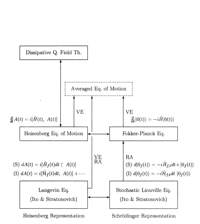
Recently we succeeded to construct a unified framework of the canonical operator

for-malism for quantum stochastic differential equations within Non-Equilibrium Thermo

FieldDynamics (NETFD) $[1]-[9]$ for the first timeto put all the formulations of

stochas-tic differential equations for quantum systems, i.e., the Langevin equation and the

stochastic Liouville equation [10] together $\mathrm{w}\mathrm{i}\mathrm{t}^{-}\mathrm{h}$ corresponding quantum master

equa-tion, into a unified method (see Fig. 1). It was possible only within the formalism of

NETFD.

In this paper, we will show that the time evolution ofa dissipative system can be

interpreted as a traverse ofthe system in a set of the unitarily inequivalent

represen-tation spaces. We believe that the set constitutes a measured space which corresponds

to the $\Gamma$ phase-space of classical

statistica,1

mechanics. We will also show that there

exists uncountable number of different descriptions of the system of quantum

differ-ential equations, and that the physical meaning of the different descriptions can be

attributed to how much

one

renormalized the line-width in an energyspectrum caused

by uncommutative effects ofa random force operator.

Wewilltreat in thispaper a non-stationary system of astochasticsemi-freeparticles. The hat-Hamiltonianforthe stochastic

_semi-free

field is $\mathrm{b}\mathrm{i}$-linear in

$a,$ $a^{\uparrow},$ $dF(t),$ $dF\dagger(t)$

and their tilde conjugates, and is invariant under the phase transformation $aarrow a\mathrm{e}^{i\theta}$,

and $dF(t)arrow dF(t)\mathrm{e}^{i\theta}$. Here, _$a,$ $a^{\uparrow}$ and their tilde conjugates are stochastic operators

of a relevant system satisfying the canonical commutation relation

$[a, a^{\uparrow}]=1$, $|\tilde{a},\tilde{a}^{\uparrow}]=1$, (1)

whereas $dF(t),$ $dF^{\uparrow}(t)$ and their conjugates $\mathrm{a}r\mathrm{e}$ random force operators. The tilde and

non-tilde operators are related with each other by the relations

$\langle$$1|a^{\uparrow}=\langle 1|\tilde{a}_{:}$ (2) $\langle$$|dF^{\uparrow}(t)=\langle|d\tilde{F}(t)$, (.3)

where $\langle$$1|$ and $\langle$$|$ are respectively the thermal $\mathrm{b}\mathrm{r}\mathrm{a}$-vacuum ofthe relevant system and of

Heisenberg Representation Schr\"odinger $\mathrm{R}\mathrm{e}\mathrm{p}_{\Gamma}\mathrm{e}\mathrm{S}\mathrm{e}\mathrm{n}\mathrm{t}\mathrm{a}\mathrm{t}\mathrm{i}\mathrm{o}11$

Figure 1: Structureof the Formalism. RA stands for the random

average.

VE$\mathrm{s}\mathrm{t}\mathrm{a}11\mathrm{d}_{\mathrm{S}}$for

The tilde $conjugati_{\mathit{0}}n\sim \mathrm{i}\mathrm{s}$ defined by:

$(A_{1}A_{2})^{\sim}=\tilde{\mathrm{A}}_{1}\tilde{A}_{2}$, (4) $(c_{1}A_{1}+c2A_{2})\sim=c_{1}^{*}\tilde{A}_{1}+C\tilde{A}_{2}2*$, (5)

$’(\tilde{A})^{\sim}=A$, (6)

$(A^{\uparrow})^{\sim}=\tilde{A}^{\uparrow}$, (7)

where $c_{1}$ and $c_{2}$

are

$c$-numbers. Any operator $A$ in

NETFD

is accompanied by its

partner (tilde) operator $\tilde{A}$

.

2

Representation

Space

of

Random

Force

Opera-tors

2.1

Fock’s

Space

We take the vectors:

$|t_{1},$ $t_{2},$ _$\cdots,$$t_{n} \rangle=\frac{1}{\sqrt{n!}}b\uparrow(t_{1})b^{\dagger}(t2)\cdots b^{\dagger}(t_{n})|0\rangle$, (8)

as a set ofbases for a Fock

space.

The argument $t$ represents time. The

vacuum

$|0\rangle$ is

defined by

$b(t)|0\rangle=0$

.

(9)

The annihilation and creation operators $b(t),$ $b^{\uparrow}(t)$ satisfy the canonical commutation

relation:

$[b(t), b^{\uparrow}(t^{J})]=\delta(t-\cdot. t’)$

.

(10)

The bases form an ortho-normal and complete set:

$\langle t_{1}, \cdots, t_{n}|t^{J/}1’\cdots,t_{m}\rangle=\delta_{n,m^{\frac{1}{n!}}}\sum_{)(P}\delta(t1^{-t^{J}}1)\cdots\delta(t_{n}-t)\prime n$’ (11)

$\sum_{n=0}^{\infty}(\prod_{l=1}^{n}\int^{\infty}0\ell dt)|t_{1},$_$\cdots,$$t_{n}\rangle\langle t_{1},$

$\cdots,$$tn|=I$. (12)

The Fockspace $\Gamma(\mathcal{H})$ over a Hilbert space$\mathcal{H}$ is the infinite Hilbert space directsum

$\Gamma(\mathcal{H})=\oplus_{n=0}^{\infty}’ \mathcal{H}^{\otimes n}\wedge$, where$\mathcal{H}^{\otimes n=}\wedge 0=C$, and, for $n\geq 1,$

$\mathcal{H}^{\otimes n}\wedge$

is the symmetric subspace

of the $n$-fold Hilbert space tensor product of$\mathcal{H}$ (the

Wiener-Ito

expansion).

For $|’\psi\rangle$ $\in\Gamma$(-?), we have

$|’ \psi\rangle=\sum_{n=0}^{\infty}(\prod_{\ell=1}^{n}\int^{\propto\rangle}\mathrm{o}dt\ell)|t_{1},$

$\cdots,$ $t_{n}\rangle\psi n(t_{17l}, \cdots, t)$, (13)

where $\psi_{n}(t_{1}, \cdots , t_{n})=\langle t_{1}, \cdots, t_{n}|\psi\rangle\in \mathcal{H}^{\oplus n}\wedge$. This situation is similar to the one in

quantum field theory when expanding a state in a Fock space in terms of the state

vectors in the $n$-particle subspace. In that case, $\psi_{n}$ is the wave-function of n-particle

2.2

Quantum

Brownian Motion

Introducing the operators

$B(t)= \int_{0}^{\mathrm{t}}dtb’(t’)$, $B^{\dagger}(t)=- \int_{0}^{t}dt’b^{\uparrow}(t’)$, (14)

for $t\geq 0$, we see that they satisfy

$B(\mathrm{O})=0$, $[B(s), B^{\dagger}(t)]= \min(s, t)$_{. (15)}

This shows that $B(t)$ and $B^{\uparrow}(t)$ are the operators

$\mathrm{r}\mathrm{e}\mathrm{p}\mathrm{r}\mathrm{e}\mathrm{s}\mathrm{e}\mathrm{n}\mathrm{t}\mathrm{i}\mathrm{l}$ quantum Brownian

motion $[11, 12]$.

The definition and the existence of the operators $b(t)$ and $b^{t}(t)$ are guaranteed by

Hida and Obata $[13, 14]$.

2.3

Ito’s Stochastic Product

When a stochastic integral $I(t)$:

$I(t)= \int_{0}^{t}dt’\{dB^{\mathrm{t}}(t’’)F(t)+G(t’)dB(t’)+H(t’)dt\}_{7}$’

(16)

with $t\geq 0$ exists, it

can

be written in a $\mathrm{d}\mathrm{i}\mathrm{f}\mathrm{i}\cdot \mathrm{e}\mathrm{I}^{\cdot}\mathrm{e}\mathrm{n}\mathrm{t}\mathrm{i}\mathrm{a}\mathrm{l}\mathrm{f}\mathrm{o}\mathrm{I}^{\cdot}\mathrm{m}$

$dI(t)=$

. $dB^{\uparrow}(t)F(t.).+G(t)dB(t)+H(t)dt$, $I(\mathrm{O})=0$. (17)

For

$dI_{i}(t)=dB\dagger(t)F_{i}(t)+G_{i}’(t)dB(t)+H_{i}(t)dt$_{, $I_{i}(0)=0$, (18)}

$(i=1,2)$, we have the Ito stochastic product [15]

$d(I_{1}I_{2})=dB^{\uparrow}(F_{1}I_{2}+I_{1}F_{2})+(G_{1}I_{2}+I_{1}G_{2})dB(t)+(H_{1}I_{2}+I_{1}H_{2}+G_{1}F_{2})dt$

$=dI_{1}I_{2}+I_{1}dI_{2}+dI_{1}dI_{2}$. (19)

Here we used

$dB(t)dB^{\dagger}(t)=dt$, ₍₂₀₎

which can be shown by the commutation relation $[dB(t), dB\dagger(t)]=dt$_. Note _{that the}

commutation relation is

a

consequence of (15). In precise, the Ito formula (19) is proven in the represelltation of the exponential vectors.

2.4

Thermal

Space

Now, put the above materials in the Hilbert space into the thermal space within

NETFD. The approach seems somewhat related to the one by $[16\rfloor$.

The operators representing the quantum Brownian motion annihilate the

vacuums

$|0\rangle$ and $\langle$_$0|$:

Let us introduce a set of

new

operators by the relation

$d\mathcal{B}(t)^{\mu}=\overline{B}(t)\mu\iota_{d}\text{ノ}B(t)^{\mathcal{U}}$, (22)

with the Bogoliubov transformation defined by

$\overline{B}(t)^{\mu\nu}=$

, (23) where theone particle distribution function $n(t)$ isspecified by the $\mathrm{B}\mathrm{o}\mathrm{l}\mathrm{t}\mathrm{z}\mathrm{m}\mathrm{a}\mathrm{l}\ln$ equation

$\frac{d}{dt}n(t)=-2\kappa(t)n(t)+i\Sigma^{<}(t)$. (24)

The function $\Sigma^{<}(t)$ is given when the interaction

hat-Hamiltonian

is specified. We

introduced the thermal doublet:

:

$\backslash$

’

$dB(t)^{\mu=}1=dB(t)$, $dB(t)^{\mu=2}=d\tilde{B}^{\uparrow}(t)$, $d\overline{B}(t)^{\mu=}1d=B^{\dagger}(t)$, $d\overline{B}(t)^{\mu=}2=-d\tilde{B}(t)$,

(25) and the similar doublet notations for $d\mathcal{B}(t)^{\mu}$ and $d\overline{\mathcal{B}}(t)^{\mu}$. The

new

operators annihilate

the new

vacuums

$\langle$$|$ and $|\rangle$:

$df?(t)|\rangle=0$, $d\mathcal{B}(t)|\rangle=0_{g}$. $\langle$$|d\mathcal{B}^{\mathrm{f}}(t)=0$,

$\langle$$|d\tilde{\mathcal{B}}\uparrow(t)=0$. (26)

2.5

Unitary

Inequivalence

The generator $\hat{U}$ inducing the Bogoliubov transformation (23) in the form

$dB(t)^{\mu}=[r^{-1}dB(i)^{\mu}\iota\wedge\wedge I,$ (27)

is given by

$\hat{U}=\exp[^{-\int_{0}^{\infty}}dt(n(t)+\frac{1}{2\kappa(t)}\frac{dn(t)}{dt})b\uparrow(t)\tilde{b}\dagger(t)]\exp[\int^{\infty}0\backslash tdb(t)\tilde{b}(t)]$ . (28)

Then, we see formally that

$|\rangle=\hat{U}^{arrow 1}|0\rangle$

$= \exp[-\delta(0)\int_{0}\propto td\ln(1+\frac{i\Sigma^{<}(t)}{2_{h}(t)})]$

$\exp[\int_{0}^{\infty}dt\frac{i\Sigma^{<}(t)}{2\kappa(t)+i\Sigma<(t)}b\dagger(t)\tilde{b}^{\uparrow(}t)]|0\rangle$. (29)

The

vacuum

$|\rangle$ and $\langle$$|$

can

be decomposed into an infinitedirect product ofunitarily inequivalent

vacuums:

$|\rangle=\hat{U}^{-1}|0\rangle$ $= \prod_{t=0}^{\infty}\exp[-\delta(0)\int_{t}^{t+}dtdt\mathrm{l}/\mathrm{n}(1+\frac{i\Sigma^{<}(t’)}{2\kappa(t’)})]$ $e \mathrm{x}\mathrm{p}[\int_{t}^{t+dt}dt’\frac{i\Sigma^{<}(t’)}{2\kappa(t’)+i\Sigma^{<}(t’)}b^{\uparrow(t’})\tilde{b}\dagger(t’)]|0\rangle$ $= \prod_{t=0}^{\propto)}|t,$$t+dt\rangle$, (30) $\mathrm{c}$ $\langle|=\langle 0|\hat{U}$ $= \prod_{0t=}^{\infty}\langle 0|e\mathrm{x}\mathrm{p}[\int_{t}^{t+dt}dtb’(t’)\tilde{b}(t’)]$ $= \prod_{t=0}^{\infty}\langle t,$$t+dt|$

.

(31) We see that $\langle t, t+dt|t, t+dt\rangle=1$, _(.32) $\langle t’, t’+dt|t, t+dt\rangle=\exp[-\delta(0)\int_{t}^{t+}dtdt’\mathrm{l}/\mathrm{n}(1+\frac{i\Sigma^{<}(t^{\prime/})}{2\kappa(t’)},)]$, (33)

for$t\neq t’$

.

The last equation (33) indicates theunitary _{inequivalence}between _{the Fock’s}

spaces labeled $t,$$t+dt$ and $t’,$$t’+dt$

.

2.6

Random Force Operators

In the following,

we

will use the representation space constructed on the

vacuums

$\langle|$

and $|\rangle$. Then,

we

have, for example,

$\langle|dB^{\mathrm{t}}(t)dB(t)|\rangle=(n(t)+\frac{1}{2\kappa(t)}\frac{dn(t)}{dt})dt$,

$\langle|dB(t)dB^{\uparrow}(t)|\rangle=(n(t)+1+\frac{1}{2\kappa(t)}\frac{dn(t)}{dt})dt$, (34)

which

was

derived by inspecting $\langle|d\tilde{B}(t)dB(t)|\rangle$ with the help of the thermal state

conditions (26).

For a practical $\mathrm{c}\mathrm{o}\mathrm{n}\mathrm{e}\mathrm{n}\mathrm{i}\mathrm{e}\mathrm{l}\mathrm{l}\mathrm{c}e$, we $\mathrm{i}_{11\mathrm{t}\mathrm{r}}\mathrm{o}\mathrm{d}\mathrm{u}\mathrm{c}\mathrm{e}$ the random force

operators by

Then,

we

have $\langle dF(t)\rangle=\langle d\tilde{F}(t)\rangle=\langle dF\dagger(t)\rangle=\langle d\tilde{F}^{\uparrow}(t)\rangle=0$, and

$\langle dF^{\uparrow}(t)dF(_{S})\rangle=(2\kappa(t)n(t)+\frac{dn(t)}{dt})\delta(t-s)dtds$,

$\langle dF(t)dF^{\dagger}(\mathit{8})\rangle=(2\kappa(t)(n(t)+1)+\frac{dn(t)}{dt})\delta(t-S)dtds$, (36)

and

zero

forothercombinations (see (34)). Here we introduced

an

abbreviation $\langle\cdots\rangle=$

$\langle|\cdots|\rangle$

.

The thermal state condition (26) reads

$(1+n(t)+ \frac{1}{2\kappa(t)}\frac{dn(t)}{dt})dF(t)|\rangle=(n(t)+\frac{1}{2\kappa(t)}\frac{dn(t)}{dt}\mathrm{I}^{d\tilde{F}}\dagger(t)|\rangle$, (37)

and (3).

3

Stochastic

Semi-Fkee System

3.1

Model

A non-stationary stochasticsemi-free system (astochastic model of a damped harmonic

oscillator) is specified by the stochastic Liouvilie equation of$\mathrm{s}_{\mathrm{t}\mathrm{I}\mathrm{a}}\mathrm{t}\mathrm{o}\mathrm{n}\mathrm{o}\mathrm{v}\mathrm{i}\mathrm{C}\mathrm{h}\mathrm{t}\mathrm{y}\mathrm{P}^{\mathrm{e}:}$

$d|0_{f}(t)\rangle=-i\hat{H}_{f,t}dt\circ|0_{f}(t)\rangle$, (38)

with the stochastic hat-Hamiltonian

$\hat{H}_{f,t}dt=\hat{H}_{S,t}dt+i\hat{\Pi}_{R,t}dt+dl\hat{\mathcal{V}}I_{t}$ (39) $=\hat{H}_{S,t}dt+[\alpha^{\mathrm{p}}(id\alpha+[\hat{H}s,\mathrm{t}dt, \alpha])-\mathrm{t}.\mathrm{c}.]$ , (40)

where the operator $\hat{\Pi}_{R,t}$ representing a relaxation effect, the martingale

$d\hat{M}_{t}$ and the

flow operators $d\alpha,$ $d\tilde{\alpha}$

are

specified, respectively, by

$\hat{\Pi}_{R,t}=-\kappa(t)(\alpha^{*}\alpha+\mathrm{t}_{\mathrm{C}}..)$, (41)

$d\hat{M}_{t}=i(\alpha^{*}dW(t)+\mathrm{t}.\mathrm{c}.)$ , (42)

$da=i[\hat{H}_{S,t}dt, \alpha]-\kappa(t)\alpha dt+dW(t)$ , (43)

and its tilde conjugate.

We introduced a set of$\mathrm{c}\mathrm{a}11\mathrm{o}\mathrm{n}\mathrm{i}_{\mathrm{C}}\mathrm{a}1$ stochastic operators

with$\mu+\nu=1$, which satisfy the commutation relation

$[\alpha, \alpha^{*}]=1$. (45)

The random force operators $dW(t),$$d\tilde{W}(t)$ are of the quantum stochastic Wiener

process satisfying

$\langle dW(t)\rangle=\langle d\tilde{W}(t)\rangle=0$, (46)

$\langle dW(t)dW(S)\rangle=\langle d\tilde{W}(t)d\tilde{W}(S)\rangle=0$, (47)

$\langle dW(l)d\tilde{W}(S)\rangle=\langle d\tilde{W}(s)dW(t)\rangle$

$=(2 \kappa(t)(n(t)+\nu)+\frac{dn(t)}{dt}\mathrm{I}^{\delta(t-}S)dtdS$, (48)

where the random force operator $dW(t)$ is defined by

$dW(t)=\mu dF(t)+\nu d\tilde{F}^{\dagger}(t)$, (49)

with $\mu+\nu=1$. The original random force operators $dF(t)$ and $dF\dagger(t)$

are

of the

non-stationary Gaussian white process derived in the previous section.

Within the stochastic

convergence,

these correlations reduce $\mathrm{t}\mathrm{o}^{1}$

$dW(t)=d\tilde{W}(t)=0$_{, (51)}

$dW(t)dW(s)=d\tilde{W}(t)d\tilde{W}(s)=0$_{, (52)}

$dW(t)d\tilde{W}(s)=d\tilde{W}(s)dW(t)$

$=(2 \kappa(t)(n(t)+l\text{ノ})+\frac{d?\tau(t)}{dt})\delta(t-s)dtds$

$=(i\Sigma^{<}(t)+2\nu\kappa(t))\delta(t-s)dtds$. (53)

We introduced the symbol $\circ$ in order to indicate the Stratonovich stochastic

multipli-cation [17].

The quantum stochastic Liouville equation (38) preserves the characteristics of the stochastic Liouville equation [10] of classical systems, i.e., the stochastic distribution

function satisfies the conservation of probability within the phase space of a relevallt

system. This means in NETFD that

$\langle 1|0_{f}(t)\rangle=1$, (54)

leading to

$\langle$$1|\hat{H}_{ft})dt=0$

.

(55)

Here the thermal $\mathrm{b}\mathrm{r}\mathrm{a}$-vacuum

$\langle$$1|$ is of the relevant system.

lForequal $\mathrm{t}\mathrm{i}_{1}\mathrm{n}\mathrm{e}t--^{s},$ (53) reads

3.2

Quantum

Langevin Equations

Forthedynamical quantity$A(t)$ ofthe relevant system, thequantum Langevin equation

of the

Stratonovich

type is given by the stochastic Heisenberg equation as [4]

$dA(t)=i[\hat{H}_{f}(t)dt^{\mathrm{o}}, A(t)]$ (56)

$=i[\hat{H}_{S}(t), A(t)]dt$

$+\kappa(t)\{[\alpha^{*}(t)\alpha(t), A(t)]+[\tilde{\alpha}^{+}\cap(t)\tilde{\alpha}(t), A(t)]\}dt$

$-\{[\alpha^{*}(t), A(t)]\circ dW(t)+[\tilde{\alpha}(+t), A(t)]\circ d\tilde{W}(t)\}$.

(.57)

3.3

Solving the

Stochastic Liouville Equation

The quantum stochastic Liouville equation of the present system in the Ito type

ex-pression is given by

$d|0_{f(t})\rangle=-i\hat{\mathcal{H}}_{f,t}dt|0_{f}(t)\rangle$, (58)

with

$\hat{\mathcal{H}}_{f,t}dt=\hat{H}_{t}dt+d\hat{M}_{t}$, (59)

where $\hat{H}_{t}$ is given by

$\hat{H}_{t}=\hat{H}_{S,t}+i\Pi_{t}\wedge$. (60) Here, $\hat{\Pi}_{t}$ is defined by $\hat{\Pi}_{t}\Rightarrow\hat{\Pi}_{R,t}+\hat{\Pi}_{D,t}$, (61) with $\hat{\Pi}_{D.t}=2(\kappa(t)(n(t)+l\text{ノ})+\frac{dn(t)}{dt}\mathrm{I}^{a}**\tilde{\alpha}.$ (62)

The diffusive time-evolution operator $\hat{\Pi}_{D,t}$ contains the information how much the

unitarily inequivalent Fock’s spaces for the random force operators overlaps with each

other in the time axis.

Note that the orthogonality

$\langle|d\hat{M}_{\mathrm{t}}|\mathrm{o}_{f}(t)\rangle=0$. (63)

3.4

Fokker-Planck

Equation

Taking the random average of the stochastic Liouville equation (58), we obtain the

Fokker-Planck equation

$\frac{\partial}{\partial t}|0(t)\rangle=-i\hat{H}t|0(t)\rangle$, (64)

with $|0(t)\rangle=\langle|0_{f}(t)\rangle$

.

It can be solved to give

The creation operators $\gamma^{*}$ and $\tilde{\gamma}^{\#_{\mathrm{a}\mathrm{r}}}\mathrm{e}$defined through

$\alpha^{\mu}=\gamma^{\nu}$, (66)

with the thermal doublet:

$\gamma^{\mu=1}=\gamma_{t}$, $\gamma^{\mu=2}=\tilde{\gamma}^{*}$, $\overline{\gamma}^{\mu=1}=\gamma^{*}$, $\overline{\gamma}^{\mu=2}=-\tilde{\gamma}_{t}$, (67) and the similar definition for $\alpha^{\mu}$. These creation and annihilation operators annihilate

the

vacuurns:

$\gamma_{t}|0(t)\rangle=0$, $\tilde{\gamma}_{\mathrm{t}}|0(t)\rangle=0$, $\langle$$1|\gamma^{*}=0$, $\langle$$1|\tilde{\gamma}^{*}=0$. (68)

The solution (65) of the Fokker-Planck equation shows that the dissipative time

evolution of the relevant systemcanbe interpreted asa condensation of$\gamma^{+}\tilde{\gamma}^{*}\backslash$-pairs into

the thermal vacuum.

4

Renormalization of the

Uncommutative

Part of

the

Random

Force Operators

We introduce here the generalized stochastic hat-Hamiltonian ofthe Stratonovich type

by

$\hat{H}_{f,t}^{\lambda}dt=\hat{H}_{S,t}dt+i\lambda\hat{\Pi}_{R,t}dt+d\hat{M}_{i}^{\lambda}$, (69)

with

$d\mathit{1}\hat{\mathcal{V}}I_{t}^{\lambda}=i\{[\alpha^{*}dW(t)+\mathrm{t}.\mathrm{c}.]-(1-\lambda)[\alpha dW^{*}(t)+\mathrm{t}.\mathrm{c}.]\}$, (70)

where $\lambda$ is a real number satisfying _{$0\leq\lambda\leq 1$}.

In addition to the random force operators $dW(t)$ and its tilde conjugate, we need

to introduce

$dW^{*}(t)=dF^{\uparrow}(t)-d\tilde{F}(t)$, (71)

and its tilde conjugate which annihilate the $\mathrm{k}\mathrm{e}\mathrm{t}$-vacuum $\langle$$|$:

$\langle$$|dW^{*}(t)=0$, $\langle$$|d\tilde{W}*(t)=0$. (72)

The additional random force operators satisfy

$dW^{*}(t)=d\tilde{W}^{*}(t)=0$, $dW^{*}(t)dW(s)=d\tilde{W}^{*}(t)d\tilde{W}(s)=0$, (73)

$dW(t)dW\#(s)=d\tilde{W}(t)d\tilde{W}^{\not\simeq}(S)=2\kappa(t)\delta(t-S)dtds$, (74)

within the stochastic

convergence.

In the generalized description, the conservation ofthe probability is satisfied in the

form:

where $\langle\langle 1|=\langle|\langle \mathrm{I}|$.

We can show that the stochastic hat-Hamiltonian of the Ito type reduces to

$\hat{\mathcal{H}}_{f,t}dt=\hat{H}_{t}dt+d\hat{M}_{t}^{\lambda}$, (76)

$(\mathrm{c}.\mathrm{f}.,$(59)$)$. Therefore, the Fokker-Planck equation remains the

same as

(64).

When $\lambda=1$, the random force operators become commutative, leading to the

system given in the previous section.

On

the other hand, when $\lambda=0$, the

general-ized hat-Hamiltonian (69) becomes hermitian. This version is intimately related to

the approaches $\mathrm{p}e$rformed by mathematicians [11, 12, 16, 18] based on the stochastic

Schr\"odinger equation (see also [19, 20]). For the intermediate $\lambda$, the relaxation rate

function in $\lambda\hat{\Pi}_{R.t}$ is partially renormalized, i.e., $\lambda\kappa(t)$, within the Stratonovich

descrip-tion. Within the Ito description, the relaxation rate function is fully renormalized in the stochastic hat-Hamiltonian ofthe Ito type.

We can interpret that the translation to the Ito description is to orthogonalize the

martingale part to the

thermal

vacuum, and to renormalize the spectrum of the

semi-free particle to have an observable (physical) line-width.

5

Summary

We showed that the time evolution of

a

dissipative system

can

be interpreted as

a

traverse ofthe system in a set of the unitarily inequivalent representation spaces. We

believe that the set constitutes a measured space which corresponds to the $\Gamma$

phase-space ofclassical statistical mechanics. Now, we

are

trying to input a

measure

into the

space which

may

provide

us

with a

new

concept of entropy.

We also showed that there exists uncountable number of different descriptions of

the system of quantum differential equations, and that the physical meaning of the

different descriptions can be attributed to how much

one

renormalized the line.width

in

an energy

spectrum caused by uncommutative effects of a random force operator.

We

are

investigating the deeper meaning ofthe renormalization within the present new

cont$e\mathrm{x}\mathrm{t}$ which was revealed only by the formalism ofNETFD.

Acknowledgment

The author would like to thallk Dr. T.

Saito

and Mr. T. Imagire for their collaboration with helpful discussions, andMessrs. T. Motoike and H. Yamazaki forfruitfulcomments.

References

[1] T. Arimitsu andH. Umezawa, Prog. Theor. Phys. 74 (1985) 429.

[2] T. Arimitsu andH.

_Umezawa:

Prog. Theor. Phys. 77 (1987) 32; 53.

[3] T. Arimitsu. Phys. Lett. A153 (1991) 163.

[5] T. Arimitsu. Lecture Note of the Summer School

_for

Younger $Phy_{\dot{\mathfrak{R}}C}\iota StS$ in Condensed Matter

Physics [published in ’ _{Bussei Kenkyu’ (Kyoto)}

60 (1993) 491, written inEnglish\rfloor .

[6] T. Arimitsu and N. $\mathrm{A}\mathrm{r}\mathrm{i}_{1}\mathrm{n}\mathrm{i}\mathrm{t}_{\mathrm{S}}\mathrm{u}$. Phys. Rev. E50

(1994) 121.

[7] T. Arimitsu. RIMS Report (Kyoto), 874 (1994) 63.

[8] T. Arimitsu. $\mathrm{c}_{\mathrm{o}\mathrm{n}}^{\mathrm{t}}\mathrm{d}\mathrm{e}\mathrm{n}\mathrm{s}\mathrm{e}\mathrm{d}$ Matter Physics (Lviv.

Ukraine) 4 (1994) 26. and thereferences therein.

[9] T. Arimitsu, RIMS Report (Kyoto), 923 (1995) 16.

[10] R. Kubo. M. Todaand N. Hashitsume. StatisticalPhysics II(Springer. Berlin 1985).

[11] R. L. Hudson and K. R. Parthasarathy, $\mathrm{C}_{01}\mathrm{n}\mathrm{n}\mathrm{l}\mathrm{u}\mathrm{n}$. Math. Phys. 93 (1984)

301.

[12] K. R. Parthasarathy, An Introduction to Quantum Stochastic $CalCul\gamma\underline{\prime}S$, Monographs in $\mathrm{M}\mathrm{a}\mathrm{t}\mathrm{l}\mathrm{u}\mathrm{e}-$

matics 85 (Birkh\"auser Verlag. 1992).

[13] N. $\mathrm{O}\mathrm{b}\mathrm{a}\mathrm{t}\mathrm{a}_{i}$Bussei Kenkyu 62 (1994) 62. in Japallese.

[14] N. Obata, RIMS Report (Kyoto) 874 (1994) 156., and thereferences therein.

[15] K. Ito, Proc. Imp. Acad. Tokyo 20 (1944) 519.

[16] R. L. Hudson and J. M. Lindsay, Ann. Inst. H. Poincar\‘e43 (1985) 133.

[17] R. Stratonovich. J. SIAM Control 4 (1966) 362.

[18] L. Accardi. Rev. Math. Phys. 2 (1990) 127.

[19] T. Saito. A System

_of

Quantum Stochastic

_Differential

Equations in te7Vns

_of

Non-Equikb$r\dot{\mathrm{v}}u$

’

Therrno Field Dynamics. Ph. D. Thesis (University ofTsukuba. 1995) unpublished.

[20] T. Saitoand T. $\mathrm{A}\mathrm{r}\mathrm{i}_{1}\mathrm{n}\mathrm{i}\mathrm{t}_{\mathrm{S}}\mathrm{u}$. (1996)