JAIST Repository: Numerical evaluation of electron repulsion integrals for pseudoatomic orbitals and their derivatives

Japan Advanced Institute of Science and Technology

JAIST Repository

https://dspace.jaist.ac.jp/

Title

Numerical evaluation of electron repulsion

integrals for pseudoatomic orbitals and their

derivatives

Author(s)

Toyoda, Masayuki; Ozaki, Taisuke

Citation

Journal of Chemical Physics, 130(12):

124114-1-124114-7

Issue Date

2009-03-25

Type

Journal Article

Text version

publisher

URL

http://hdl.handle.net/10119/10840

Rights

Copyright 2009 American Institute of Physics.

This article may be downloaded for personal use

only. Any other use requires prior permission of

the author and the American Institute of Physics.

The following article appeared in Masayuki Toyoda

and Taisuke Ozaki, Journal of Chemical Physics,

130(12), 124114 (2009) and may be found at

http://dx.doi.org/10.1063/1.3082269

Numerical evaluation of electron repulsion integrals for pseudoatomic

orbitals and their derivatives

Masayuki Toyoda and Taisuke Ozaki

Citation: J. Chem. Phys. 130, 124114 (2009); doi: 10.1063/1.3082269

View online: http://dx.doi.org/10.1063/1.3082269

View Table of Contents: http://jcp.aip.org/resource/1/JCPSA6/v130/i12

Published by the American Institute of Physics.

Additional information on J. Chem. Phys.

Journal Homepage: http://jcp.aip.org/

Journal Information: http://jcp.aip.org/about/about_the_journal

Top downloads: http://jcp.aip.org/features/most_downloaded

Numerical evaluation of electron repulsion integrals for pseudoatomic

orbitals and their derivatives

Masayuki Toyodaa兲 and Taisuke Ozaki

Research Center for Integrated Science, Japan Advanced Institute of Science and Technology, 1-1, Asahidai, Nomi, Ishikawa 932-1292, Japan

共Received 29 December 2008; accepted 27 January 2009; published online 25 March 2009兲 A numerical method to calculate the four-center electron-repulsion integrals for strictly localized pseudoatomic orbital basis sets has been developed. Compared to the conventional Gaussian expansion method, this method has an advantage in the ease of combination with O共N兲 density functional calculations. Additional mathematical derivations are also presented including the analytic derivatives of the integrals with respect to atomic positions and spatial damping of the Coulomb interaction due to the screening effect. In the numerical test for a simple molecule, the convergence up to 10−5 _{hartree in energy is successfully obtained with a feasible cost of}

computation. © 2009 American Institute of Physics.关DOI:10.1063/1.3082269兴

I. INTRODUCTION

In ab initio electronic structure calculations based on the density functional theory 共DFT兲, the Fock exchange for Kohn–Sham orbitals has been occasionally used as the “ex-act” exchange in order to improve the poor description of exchange energy by the Dirac exchange, which is the stan-dard functional used in the local density approximation 共LDA兲 and the generalized gradient corrections 共GGA兲. In recent years, various molecular systems have been calculated by using the hybrid functional methods,1 such as B3LYP2,3 and PBE0,4where a certain amount of the Fock exchange is admixed with the LDA/GGA exchange-correlation function-als. The introduction of the nonlocal Fock exchange signifi-cantly improves the delocalization error5 in the semilocal LDA/GGA functional and presents better thermochemical and structural properties of molecules.

The heavy computational demand to evaluate the Fock exchange is, however, a serious drawback. The studies for large molecules and solids are thus very limited. One solu-tion for this problem is given in the Heyd–Scuseria– Ernzerhof共HSE兲 hybrid functional6where the long tail of the Coulomb interaction is somewhat artificially damped. The successful application of the HSE hybrid functional to ex-tended systems, typified by the surprisingly accurate values of the band-gap energies of semiconductors,7implies that the damping scheme they introduced is not just conducive to reducing the computational cost, but reasonable as well to describe the screening of the Coulomb interaction in real materials.

The Fock exchange consists of the four-center electron repulsion integrals 共ERI兲 among basis functions. Since the integration can be performed analytically with the Gaussian-type orbital 共GTO兲 basis functions, the Gaussian-expansion method is conventionally used in the evaluation of ERI where the basis functions are expanded in terms of GTO

basis set.8–10However, the Gauss transform of a numerically defined function might require an indirect way such as a fitting process of the function to analytic functions unlike that for the Slater-type orbital 共STO兲 functions.8 While, in our method, ERI is evaluated directly from arbitrarily de-fined basis functions. Specifically in the O共N兲 DFT calcula-tion codes, such asCONQUEST,11SIESTA,12 andOPENMX,13–15 the strictly localized pseudoatomic orbital 共PAO兲 basis sets are commonly used since the real space sparsity of the re-sultant Hamiltonian and overlap matrices enable us to com-bine the scheme with various O共N兲 methods and to parallel-ize the computation by the domain decomposition in real space. Therefore, toward the implementation of the hybrid functionals or any other methods which utilizes the Fock exchange in the O共N兲 DFT calculations, an effective numeri-cal method is required to evaluate the Fock exchange for the nonanalytic PAO basis functions.

In this paper, we present a numerical procedure to cal-culate the four-center ERI for the numerically defined basis functions. We briefly review the mathematical derivations in the next section. Then, based on the formulations, we derive the analytic derivatives of the integrals with respect to atomic positions, which are required for the calculation of the forces on atoms. Our derivation is fully analytic and con-sistent with the integrals themselves. We also derive the for-mulation of ERI when the spatial damping of the Coulomb interaction is introduced as in the HSE hybrid functional.

II. FORMULATION

A. Numerical evaluation of ERI

The essential mathematical analysis described in this section is provided by Talman.16The considered wave func-tions are expressed as the linear combination of the PAO basis functions and each basis function is a product of a numerically defined radial function f共r兲 and an eigenfunction of angular momentum, i.e., the spherical harmonic function

YL共rˆ兲 for given angular momentum L=共ᐉ,m兲, a兲_{Author to whom correspondence should be addressed. Electronic mail:}

[email protected].

THE JOURNAL OF CHEMICAL PHYSICS 130, 124114共2009兲

␸共r兲 = f共r兲YL共rˆ兲. 共1兲

The Fock exchange for the wave functions is then expressed as the sum of ERI for the basis functions. In general, ERI for four basis functions centered at different positions, a1, a2, a3

and a4, is defined as follows:

I4⬅

冕冕

␸1ⴱ共r − a1兲␸2共r − a2兲

⫻ 1

兩r − r

⬘

兩␸3共r

⬘

− a3兲␸4ⴱ共r

⬘

− a4兲d3rd3r

⬘

. 共2兲

I₄ is also denoted as 共␸₁␸₂兩␸₃␸₄兲 to make the order of the basis functions clear. This integral is quite difficult to com-pute since the integration has to be performed over six-dimensional space coordinates. To reduce the six-dimensionality of the coordinates, one first needs to describe the overlap of the basis functions,␸₁ and␸₂, as a function centered at an arbitrarily chosen center c, which will be referred to as the overlap function later, and, similarly, the overlap of␸₃ and ␸4at another center c

⬘

,

F12共r − c兲 =␸1共r − a1兲␸2ⴱ共r − a2兲, 共3兲

F34共r − c

⬘

兲 =␸3共r − a3兲␸4ⴱ共r − a4兲. 共4兲

Then, the integral Eq.共2兲becomes

I4=

冕冕

共F12共r − c兲兲ⴱ

1

兩r − r

⬘

兩F34共r

⬘

− c

⬘

兲d3rd3r

⬘

. 共5兲 By using the Fourier transform of the Coulomb interaction 1/r,

冕

eik·r r d

3_{r =}4␲

k2 , 共6兲

the integral in reciprocal space is expressed as a single-center integral, I₄= 1 2␲2

冕

1 k2共F˜ 12_共k兲兲ⴱ_F˜34_共k兲eik·R_d3_{k, 共7兲}

where R⬅c

⬘

− c and F˜ij are the Fourier transformed func-tions of Eqs.共3兲and共4兲. Since F˜ij_{is also expanded in terms}

of the spherical harmonic functions,

F ˜ij_{共k兲 = 4␲}

兺

L iᐉP˜L ij_共k兲Y L共kˆ兲, 共8兲

the angular part of the integral in Eq. 共7兲can be performed analytically, where the overlap coefficient, P˜L

ij_{共k兲, is a radial}

function of k, which will be discussed later on. Finally, the integral Eq. 共2兲 is broken down to a sum of single-dimensional integrals as follows:

I4= 32␲

兺

L

兺

_L⬘ ⌳=共␭,␮兲

兺

iᐉ⬘−ᐉ+␭G_LL_⬘⌳Q_LL␭ _⬘共R兲共Y_⌳共Rˆ兲兲ⴱ, 共9兲 Q_LL␭ _⬘共R兲 ⬅

冕

0 ⬁ j_␭共kR兲共P˜L 12_共k兲兲ⴱ_P˜ L⬘ 34_{共k兲dk, 共10兲}

where G_LL_⬘⌳is the Gaunt coefficients defined by

G_LL_⬘⌳⬅

冕

共YL共rˆ兲兲ⴱYL⬘共rˆ兲Y_⌳共rˆ兲d⍀r. 共11兲

The remaining problem is how to calculate the overlap coef-ficients P˜L

ij

in Eq. 共8兲. In order to calculate them, the trans-lation of the expansion center of a basis function is consid-ered based on the investigation by Löwdin17 as follows:

␸i共r − a兲 =

兺

⌳ ␣⌳

i_共r,a兲Y

⌳共rˆ兲. 共12兲

The coefficients ␣_⌳i, often referred to as ␣-function, are given by ␣_⌳i 共r,a兲 = 4␲

兺

⌳⬘ iᐉi−␭+␭⬘_G ⌳⌳_⬘ L_i ⌫_␭␭i _⬘ 共r,a兲Y⌳_⬘共aˆ兲, 共13兲

with a function of r and a defined by ⌫_␭␭i _⬘

共r,a兲 = 2

␲S共␭兲关j␭⬘共ka兲f˜i共k兲兴. 共14兲

Here,S共␭兲 is the␭th order spherical Bessel transform 共SBT兲 and f˜i共k兲 is the transformed radial function given by

f˜i共k兲 = S共ᐉi兲关fi共r兲兴 ⬅

冕

0 ⬁ j_ᐉ i共kr兲fi共r兲r 2_{dr. 共15兲}

The overlap functions, Eqs. 共3兲 and 共4兲, are described in terms of␣-functions关Eq.共13兲兴:

Fij共r兲 =␸i共r − 共ai− c兲兲␸ⴱj共r − 共aj− c兲兲 =

兺

L PL ij_共r,a i− c,aj− c兲YL共rˆ兲, 共16兲 where PL ij_共r,a i− c,aj− c兲 =

兺

⌳

兺

_⌳⬘ G_⌳⌳_⬘L␣_⌳i共r,ai− c兲共␣_⌳⬘ j 共r,aj− c兲兲ⴱ. 共17兲 Finally, by transforming Eq.共17兲, the overlap coefficients in reciprocal space are obtained as

P ˜ L ij_{共k兲 = S共ᐉ兲关P} L ij_共r,a i− c,aj− c兲兴. 共18兲

Let us summarize how to compute ERI in the present approach: The first step is to transform the radial part of the basis functions by Eq.共15兲. Then, for every pair of orbitals, ␣-functions are calculated through Eqs.共13兲and共14兲. From those␣-functions, the overlap coefficients关Eq.共17兲兴 and the transformed ones关Eq.共18兲兴 are obtained. Finally, the integral 关Eq. 共9兲兴 is calculated by summing up the radial integrals 关Eq. 共10兲兴.

B. Fast spherical Bessel transform

In the above approach, the SBT is performed at three different places, namely, Eqs.共14兲,共15兲, and 共18兲. Since the orders of the transforms are different and high at each step, this process can be a source of numerical errors as well as a bottleneck in the computation speed. A careful examination is therefore required in implementing the numerical method of SBT.

In the preceding works by Talman, the fast SBT tech-nique is used, which is proposed by Siegman18and Talman.19 In our experience of testing several numerical techniques, such as the discrete Bessel transform20 and the asymptotic expansion method,21 we reached the conclusion that the Siegman–Talman fast SBT method is actually the most stable and fast for the present approach.22It, however, still suffers from oscillating numerical error in high-order transforms. The error becomes more significant for the PAO basis func-tions than the analytic basis funcfunc-tions because of their finite truncation. Fortunately, the oscillating error can be substan-tially suppressed by applying a simple correction to the fast SBT method as we describe later in this section.

In the fast SBT method, the radial variables r and k are changed to their logarithms,

␳= ln共r兲, ␬= ln共k兲. 共19兲

Then SBT of a function f共r兲 with order ᐉ,

f˜共k兲 = S共ᐉ兲关f共r兲兴 ⬅

冕

0 ⬁

j_ᐉ共kr兲f共r兲r2dr, 共20兲

becomes a convolution-type integral as follows:

f˜共k兲 = f˜共e␬兲 = e共m−3/2兲␬F关M_ᐉ,m共t兲F关e共m+3/2兲␳f共e␳兲兴兴, 共21兲

where m = 0 , 1 , 2 , . . . ,ᐉ is an arbitrarily chosen parameter and

F is the Fourier transform.

The function M_ᐉ,m共t兲 is the Fourier transformed spherical Bessel function,

M_ᐉ,m共t兲 = 1

2␲

冕

_−⬁

⬁

e−it␳e共3/2−m兲␳j_ᐉ共e␳兲d␳, 共22兲 where the integral can be performed analytically.19The trans-form, Eq. 共21兲, is thus reduced to a couple of consecutive one-dimensional Fourier transforms, where we can take ad-vantages of the speed of the fast Fourier transform algorithm.

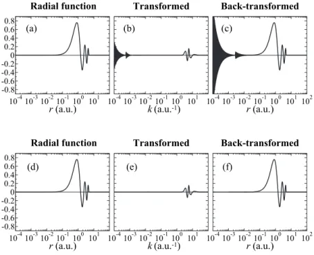
As mentioned before, the fast SBT method suffers from the oscillating numerical error in high-order transforms. In Fig. 1, a typical example of such error is shown, where a PAO basis function is transformed with the order ᐉ=14 and

m = 0, and then back transformed with the same order. In the

transformed function 共the upper middle panel兲, the oscillat-ing error appears in the small-k region. After the back-and-forth transform 共the upper right-hand panel兲, the accumula-tion of error is observed. Often, the error approaches quickly to infinity and the computation crashes.

In order to avoid the error, a simple correction is applied. Since the error appears only in the small-k region, we per-form the integration of Eq. 共20兲 for some selected k-points between 0 and k0 by using the straightforward trapezoidal

method, where k0 is smaller than the smallest k-points used

in the final integration Eq. 共10兲so that the effect of the cor-rection can be negligible, but the numerical breakdown can be avoided. By a linear interpolation between the selected

k-points, we obtain another transformed function g˜共k兲, in

ad-dition to f˜共k兲. Then we replace f˜共k兲 with g˜共k兲 for k⬍k0 as

follows:

f˜corrected共k兲 = f˜共k兲⌰共k − k0兲 + g˜共k兲⌰共k0− k兲. 共23兲

This rather crude way of correction actually serves the prac-tical purpose. The lower panels of Fig. 1show the example of the back-and-forth transform of the PAO basis function with the corrected fast SBT. Here, we use k0= 10−2 and the

straightforward integrations are performed only for three se-lected k-points, which are k0, 10−4, and 0. It is confirmed that

the oscillating error is successfully suppressed.

C. Derivatives

For the calculation of forces acting on atoms, we derive the derivatives of the integral Eq.共9兲with respect to atomic FIG. 1. Accumulation of numerical error by back-and-forth transforms with the fast SBT method. The input function共a兲 is a PAO orbital of H atom for ᐉ=2 and

n_node= 4. The transformed function of共a兲 is plotted in the panel共b兲 and the back-transformed of 共b兲 is in panel 共c兲. In the lower panels 共d兲, 共e兲, and 共f兲, accumulation of numerical error by back-and-forth transforms with our modified fast SBT method is shown, where the error is substantially suppressed.

positions. In our derivation, the expansion centers for the overlap functions are assumed to be given by the following forms:

c = pa₁+共1 − p兲a₂, 共24兲

c

⬘

= p

⬘

a3+共1 − p

⬘

兲a4, 共25兲

where 0ⱕp共p

⬘

兲ⱕ1. Having in mind that R=c

⬘

− c, the de-rivatives are obtained as

⵱a₁I4= 32␲

兺

LL⬘⌳ iᐉ⬘−ᐉ+␭G_LL_⬘⌳共− pA + B12兲, 共26兲 ⵱a₂I4= 32␲

兺

LL⬘⌳ iᐉ⬘−ᐉ+␭G_LL_⬘⌳共− 共1 − p兲A − B12兲, 共27兲 ⵱a₃I4= 32␲

兺

LL⬘_⌳ iᐉ⬘−ᐉ+␭GL⬘_⌳ L 共p

⬘

A + B34兲, 共28兲 ⵱a₄I4= 32␲

兺

LL⬘⌳ iᐉ⬘−ᐉ+␭G_LL_⬘⌳共共1 − p

⬘

兲A − B34兲, 共29兲

where the vectors A, B12, and B34 are defined as A⬅ AY_⌳共Rˆ兲eR+ QLL⬘ ␭ _共R兲 ⫻

冉

1 R ⳵Y_⌳共Rˆ兲 ⳵␪ e␪+ 1 R sin␪ ⳵Y_⌳共Rˆ兲 ⳵␾ e␾

冊

, 共30兲 A⬅

冕

0 ⬁ k

冉

d dzj␭共z兲

冊

z=kR 共P˜L 12_共k兲兲* P ˜ L⬘ 34_{共k兲dk, 共31兲} B12⬅

冕

0 ⬁ j_␭共kR兲共⵱a₁˜PL 12_共k兲兲* P ˜ L⬘ 34_{共k兲dk, 共32兲} B₃₄⬅

冕

0 ⬁ j_␭共kR兲共P˜L12共k兲兲*共⵱a₃P˜L⬘ 34_{共k兲兲dk. 共33兲}

Here, the unit vectors are defined as follows:

eR⬅ 共sin␪cos␾, sin␪sin␾, cos␪兲, 共34兲

e_␪⬅ 共cos␪cos␾, cos␪sin␾, − sin␪兲, 共35兲

e_␾⬅ 共sin␾, cos␾, 0兲, 共36兲

where ␪ and ␾ are the spherical coordinate components of the vector R.

The vector A can be calculated immediately since all the differentiations in Eqs. 共30兲and 共31兲are taken for the ana-lytic functions. As shown in the Appendix, the differentia-tions of the overlap funcdifferentia-tions in Eqs.共32兲and共33兲can also be performed completely analytically. Note that the differen-tiations are taken only for a1 and a3 because the others can

also be obtained via the following sum rule:

⵱a₁P˜L12共k兲 + ⵱a₂P˜L12共k兲 = 0, 共37兲

⵱a₃P˜L

34_{共k兲 + ⵱}

a₄P˜L

34_{共k兲 = 0. 共38兲}

The rule arises due to the assumption of Eqs.共24兲 and共25兲 and this is the reason why we assumed them. There is an-other sum rule,

⵱a₁I4+⵱a₂I4+⵱a₃I4+⵱a₄I4= 0, 共39兲

which is a more general one arising from the definition of the integral. It is easily confirmed that the derivatives, Eqs. 共26兲–共29兲, satisfy the rule.

D. Screening of the Coulomb interaction

We also derive the formulation of ERI when the screen-ing of Coulomb interaction is introduced. The screenscreen-ing scheme is assumed to be the same with that used in the HSE hybrid functional,6

1

r→

1 − erf共␻r兲

r , 共40兲

where erf共␻r兲 is the Gauss error function and␻is a screen-ing parameter. The Fourier transform of the screened Cou-lomb interaction is

冕

1 − erf共␻r兲 r e ik·r_d3_{r =}4␲ k2共1 − e −k2/4␻2_{兲. 共41兲}

Therefore, the radial integral关Eq.共10兲兴 becomes TABLE I. Definition of the integrals in the calculations of ERI for GTO.

Integral Function Radial Angular 共ss兩ss兲 ␸1,␸2,␸3,␸4 e−r Y00= 1/冑4␲ 共ps兩sp兲 ␸2,␸3 e−r Y00= 1/冑4␲ ␸1 re−r Y1−1=冑3/8␲共x−iy兲/r ␸4 re−r Y11= −冑3/8␲共x+iy兲/r 共dd兩dd兲 ␸1 r2e−r/2 Y2 2₌冑_15/32␲共x2_{− y}2_{+ 2ixy兲/r}2 ␸2 r2e−r/2 Y2 −1₌冑_{15/8␲共xz−iyz兲/r}2 ␸3 r2e−r/2 Y2 1_{= −}冑_{15/8␲共xz+iyz兲/r}2 ␸4 r2e−r/2 Y2−2=冑15/32␲共x2− y2− 2ixy兲/r2

TABLE II. Convergence of the calculations of ERI for GTO basis set with respect to the cutoff parameterᐉmax.

ᐉmax Integrals 共hartree兲 共ss兩ss兲 共ps兩sp兲 共dd兩dd兲 0 0.007 608 0.002 853 0.000 000 1 0.002 384 0.001 055 2 0.002 512 0.000 305 3 0.002 656 4 ⫺0.001 909 5 ⫺0.001 909 6 ⫺0.001 965 exact 0.007 608 0.002 512 ⫺0.001 966

Q_LL␭,scr_⬘共R兲 =

冕

j_␭共kR兲共P˜L 12_共k兲兲* P ˜ L⬘ 34_{共k兲共1 − e}−k2/4␻2_兲dk. 共42兲 Since the screening factor is independent of the atomic po-sitions, the derivatives are still in the similar forms as Eqs. 共26兲–共29兲, except, the radial integrals Eqs. 共31兲–共33兲are re-placed with the screened ones as follows:

Ascr共␻兲 ⬅

冕

0 ⬁ k

冉

d dzj␭共z兲

冊

z=kR 共P˜L 12_共k兲兲* P ˜ L⬘ 34_共k兲 ⫻共1 − e−k2/4␻2_{兲dk, 共43兲} B₁₂scr共␻兲 ⬅

冕

0 ⬁ j_␭共kR兲共⵱a₁P˜L 12_共k兲兲* P ˜ L⬘ 34_{共k兲共1 − e}−k2/4␻_兲dk, 共44兲 B₃₄scr共␻兲 ⬅

冕

0 ⬁ j_␭共kR兲共P˜L12共k兲兲*共⵱a₃P˜L⬘ 34_共k兲兲 ⫻共1 − e−k2/4␻2_{兲dk. 共45兲} E. Computation speed

Our motivation is in the application of the Fock ex-change in large systems such as large molecules and solids. In those systems, an enormous共infinite for solids兲 number of combinations of basis functions have to be considered. For-tunately for the PAO basis sets, since they are strictly con-fined in real space, the overlaps are exactly zero whenever the distance between the basis functions is longer than the sum of the confinement lengths. On the other hand, however, any two overlap functions can interact with each other even if they are separated quite far apart because of the infinitely long tail of the Coulomb interaction. By using the screening scheme described in the previous section, it might be justi-fied to neglect the contribution from the far-separated pairs. Nevertheless, still a large number of pairs have to be calcu-lated since the typical value of the screening parameter is ␻= 0.15a−1 and thus the effective screening length is ⬃10 Å.7

Therefore, we should consider making the compu-tation faster for the final integration关Eqs. 共9兲and共10兲兴. As already pointed out by Talman, the convergence of the

sum-mation Eq.共9兲is very fast so that the cutoff angular momen-tum ᐉmax and the number of k-sampling points Nk can be

decreased. We shall define new parametersᐉmax and N¯k for

Eqs. 共9兲 and 共10兲 in order to distinguish from the original parameters ᐉmax and Nk, which are used in the other parts.

Typically, ᐉmax has to be as large as ⬃15 to describe the

overlap functions accurately. While, as shown later,ᐉmax= 6

is enough to obtain 10−5 hartree accuracy in energy even when d orbitals are involved. Similarly, Nkis required to be

⬃1000, while in the final integration, the Gauss–Laguerre quadrature can be used, which gives good convergence with

N¯k⬃50.

The location of the expansion centers c has also a sig-nificant effect on the convergence speed. In general, c is an orbital-dependent value. Therefore, since ␣-functions Eqs. 共13兲and共14兲depend on c关note that what we actually need is the terms in the right-hand side of Eq. 共17兲兴, one needs to calculate those coefficients of which the number is equiva-lent to that of neighboring orbitals. Here, we offer a sugges-tion that the computasugges-tion cost may be reduced by choosing c at the middle of the two orbital centers,

c =a1+ a2

2 . 共46兲

In this case, the required number of␣-functions is decreased by a factor of the number of orbitals per atom, which is typically⬃10. Note that Eq.共46兲is not the best choice if just one ERI is considered. In fact, the choice of c considering the spatial extent of each orbital gives faster convergence in the final integration.23 Therefore, it becomes a competition between the convergence speed in performing a single inte-gral and the required number of␣-functions.

III. COMPUTATION RESULTS

In order to check the convergence properties of our rou-tine, we first performed calculations of ERI for a GTO basis set. Three different integrals 共ss兩ss兲, 共ps兩sp兲, and 共dd兩dd兲 are calculated. The definition of the basis functions for the integrals is listed in TableI. For all the integrals, the orbital locations are fixed to the corners of a square on the x-y plane with edge length of 1; a1=共1/2,1/2,0兲, a2=共1/2,−1/2,0兲, a3=共−1/2,1/2,0兲, and a4=共−1/2,−1/2,0兲. The cutoff for

the angular momentum isᐉmax= 15 and the number of radial

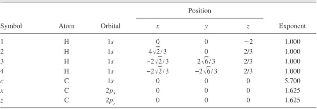
mesh points is N = 1024. In the final integration, the Gauss– TABLE III. Basis functions and atomic positions in the calculations of methane molecule. The STO basis

functions are normalized.

Symbol Atom Orbital

Position Exponent x y z 1 H 1s 0 0 ⫺2 1.000 2 H 1s 4冑2/3 0 2/3 1.000 3 H 1s −2冑2/3 2冑6/3 2/3 1.000 4 H 1s −2冑2/3 −2冑6/3 2/3 1.000 c C 1s 0 0 0 5.700 x C 2px 0 0 0 1.625 z C 2py 0 0 0 1.625

Laguerre quadrature is used where the number of k-sampling points is N¯k= 60 and the summation is taken up to a reduced

cutoffᐉmax. In TableII, the calculated values of the integrals

are shown for increasingᐉmax, where they are left blank after

the convergence up to 10−5 hartree is achieved. The exact values are also shown for comparison, which are obtained by using the analysis given in literature.9It is clearly found that the convergence becomes slower for orbitals with higher an-gular momentum. Nevertheless, the accurate values for all the integrals up to 10−5 hartree are obtained withᐉmax= 6.

As a more realistic example, we performed calculations of ERI of a methane molecule for a STO basis set. The basis functions and the atomic positions are summarized in Table III. Our results and the comparison values calculated by us-ing the Gaussian expansion method9 are shown in TableIV. For all the integrals considered, ours and the comparison values agree with each other up to 10−5 _{hartree. The}

differ-ence from the comparison values is large for 共c1兩c2兲 and 共cc兩12兲 because the C 1s inner-shell orbital is involved. In general, the small spatial extent of such inner-shell orbitals makes the convergence slower. This, however, would not have to be considered so seriously in the actual calculations if the contributions of the inner-shell electrons are included in the pseudopotentials.

Calculations of ERI for a PAO basis set are performed for the methane structure. The PAO data are taken from those

used in theOPENMXDFT calculation package.24The ground state orbitals generated by the confinement scheme13with the radius of 5.0 bohr are used as the PAO basis functions for both the hydrogen and carbon atoms. The calculated values are shown in Table V where the parameters ᐉmax= 15, N

= 1024, and N¯k= 60 are used. The comparison values are also

calculated by using the present method with the enhanced parameters ᐉmax= 20 and N = 4096. As well as the analytic

functions such as GTO and STO basis sets, even for the strictly localized PAO basis set, it is confirmed that the con-vergence up to 10−5 _{hartree is obtained withᐉ}

max= 6.

The computation time in our method for calculating a single integral is 3.0 sec with Intel Xeon processor 3.2 GHz. This is too expensive compared to the time required in the conventional Gaussian-expansion method, e.g., one of the most sophisticated program takes only 0.5–1.3 msec per in-tegral with Intel Pentium IV processor 3.2 GHz.10 In our method, most of the time is consumed in the calculation of the overlap functions. Fortunately, the required number of pairs is proportional to the number of basis functions due to the finite truncation of the PAO basis functions, whereas the effort of the computation of ERIs scales quadratically as the number of the basis functions increases. In addition to that, the overlap functions can be reused for the calculations of ERI with a different pair of them, e.g., the overlap of 1 and 2 TABLE IV. Convergence of the calculations of ERI of methane molecule for the STO basis set. The symbols

1, 2, 3, 4, c, x, and z specify the STO basis functions of H and C atoms. See Table III for details. The comparison values are taken from Ref.9.

ᐉmax Integrals 共hartree兲 共12兩34兲 共12兩13兲 共11兩23兲 共c1兩34兲 共c1兩c2兲 共cc兩12兲 共c1兩x2兲 共c1兩z2兲 0 0.031 420 0.035 743 0.097 301 0.013 109 0.011 258 0.170 321 0.026 924 0.009 519 1 0.031 420 0.035 743 0.097 301 0.013 010 0.011 186 0.170 321 0.020 083 0.006 288 2 0.030 647 0.035 666 0.095 631 0.012 719 0.011 188 0.166 242 0.020 144 0.006 106 3 0.030 647 0.035 666 0.095 631 0.012 723 0.011 188 0.166 242 0.019 819 0.005 914 4 0.030 684 0.035 694 0.095 709 0.012 743 0.011 188 0.166 578 0.019 834 0.005 902 5 0.030 684 0.035 694 0.095 709 0.012 743 0.011 188 0.166 578 0.019 809 0.005 887 6 0.030 681 0.035 694 0.095 703 0.012 741 0.011 188 0.166 531 0.019 811 0.005 887 Comp. 0.030 683 0.035 694 0.095 706 0.012 741 0.011 195 0.166 536 0.019 809 0.005 885

TABLE V. Convergence of the calculations of ERI of methane molecule for the PAO basis set. The symbols and the atomic positions are the same as in TableIII. The comparison values are also calculated by using the present method with enhanced parameters共see text for details兲.

ᐉmax Integrals 共hartree兲 共12兩34兲 共12兩13兲 共11兩23兲 共c1兩34兲 共c1兩c2兲 共cc兩12兲 共c1兩x2兲 共c1兩z2兲 0 0.031 071 0.035 881 0.096 122 0.070 962 0.158 759 0.141 194 ⫺0.044 336 0.047 671 1 0.031 071 0.035 881 0.096 122 0.071 814 0.161 936 0.141 194 ⫺0.030 393 0.018 107 2 0.030 601 0.035 835 0.095 266 0.071 497 0.162 871 0.140 576 ⫺0.031 044 0.020 152 3 0.030 601 0.035 835 0.095 266 0.071 508 0.162 823 0.140 576 ⫺0.030 911 0.019 802 4 0.030 630 0.035 860 0.095 316 0.071 517 0.162 851 0.140 577 ⫺0.030 915 0.019 825 5 0.030 630 0.035 860 0.095 316 0.071 517 0.162 851 0.140 577 ⫺0.030 906 0.019 826 6 0.030 627 0.035 860 0.095 313 0.071 516 0.162 855 0.140 577 ⫺0.030 905 0.019 828 comp. 0.030 630 0.035 862 0.095 318 0.071 519 0.162 859 0.140 581 ⫺0.030 903 0.019 829

for共12兩34兲 can also be used for 共12兩56兲, etc. Therefore, the computation efficiency in total can be significantly enhanced as the system size becomes larger.

IV. SUMMARY

In summary, a numerical method to evaluate ERI for the PAO basis sets has been developed. Based on the mathemati-cal analysis by Talman, we derived the analytic derivatives and a spatial damping scheme for the Coulomb interaction. We also propose a numerical method for SBT of the strictly localized PAO basis functions, where the oscillating numeri-cal error is well suppressed even for the high-order trans-forms. In the numerical calculations for a simple molecule, the convergence up to 10−5 hartree in energy has been suc-cessfully obtained. The present method enables us to utilize state-of-the-art hybrid functional methods in the O共N兲 DFT calculation programs.

ACKNOWLEDGMENTS

This work was partly supported by CREST-JST and the Next Generation Super Computing Project, Nanoscience Program, MEXT, Japan.

APPENDIX: DERIVATIVES OF OVERLAP FUNCTIONS

The derivatives of the overlap functions in the vectors 关Eqs.共32兲and共33兲兴 are given as

⵱a_iP˜L ij_{共k兲 = ⵱} a_iSBTᐉ关PL共r,ai− c,aj− c; fi, fj兲兴 =

兺

⌳⌳⬘ G_⌳⌳_⬘L兵共1 − p兲共⵱u␣_⌳ i_{共r,u兲兲␣} ⌳_⬘ j 共r,v兲 − p␣_⌳j共r,u兲共⵱_v␣_⌳i_⬘共r,v兲兲其u=ai−c v=a_j−c, 共A1兲

where we use the assumption in Eqs.共24兲and共25兲. Then, the derivatives of the␣-functions are

⵱a␣_␭␩共r,a兲 = 4␲

兺

⌳⬘ iᐉ−␭+␭⬘G_⌳⌳L␩_⬘

再

冉

⳵ ⳵a⌫␭␭⬘ ␩ _共r,a兲

冊

_Y ⌳_⬘共aˆ兲er +1 a⌫␭␭⬘ ␩ _共r,a兲 ⳵ ⳵␪Y⌳⬘共aˆ兲e␪ + 1 a sin␪⌫␭␭⬘ ␩ _共r,a兲 ⳵ ⳵␾Y⌳_⬘共aˆ兲e␾

冎

, 共A2兲

where the unit vectors are similar to Eqs.共34兲–共36兲, where␪ and␾are the spherical coordinate components of a.

We come to the final equation, the derivatives of ⌫ terms, ⳵ ⳵a⌫␭␭⬘ i _{共r,a兲 =} 2 ␲SBT共␭兲

冋

冏

k

冉

d dzj␭⬘共z兲

冊

冏

_z=kaf˜ᐉ共k兲

册

. 共A3兲

As derived here, all the components are derived analytically, without using any numerical differentiation.

In Eq.共30兲, there are terms proportional to 1/R, which diverge as R approaches zero. In fact, R can be a near-zero values when, for example, atoms are on a square lattice and the orbitals␸₁and␸₂are located at each end of a diagonal of the square, and␸₃and␸₄ are at each end of the other diag-onal. To avoid such numerical problem, we impose a lower limit on R as follows:

R→ R¯ ⬅

冑

R2+␦2exp共− R2/␦2兲, 共A4兲 where␦Ⰶ1. The same problem may arise for the derivative of␣terms关Eq.共A2兲兴. However, we do not need to consider the case when a is close to zero. This is because, in such case, the two orbitals are located on a same atom and thus the derivative of the overlap function关Eq. 共A1兲兴 should al-ways be zero. Here, we assume that all the orbitals are lo-cated on the atoms. Note that the derivatives are not taken with respect to the orbital centers but to the atomic positions.

1_{A. D. Becke,J. Chem. Phys. 98, 1372共1993兲.} 2_{A. D. Becke,J. Chem. Phys. 98, 5648共1993兲.}

3_{P. J. Stephens, F. J. Devlin, C. F. Chabalowski, and M. J. Frisch,J. Phys.}

Chem. 98, 11623共1994兲.

4_{C. Adamo and V. Barone,J. Chem. Phys. 110, 6158共1999兲.}

5_{P. Mori-Sánchez, A. J. Cohen, and W. Yang, Phys. Rev. Lett. 100,}

146401共2008兲.

6_{J. Heyd, G. E. Scuseria, and M. Ernzerhof,J. Chem. Phys. 118, 8207}

共2003兲.

7_{J. Heyd and G. E. Scuseria,J. Chem. Phys. 121, 1187共2004兲.} 8_{I. Shavitt and M. Karplus,J. Chem. Phys. 36, 550共1962兲.}

9_{H. Taketa, S. Huzinaga, and K. O-ohata, J. Phys. Soc. Jpn 21, 2313}

共1966兲.

10_{J. Fernández Rico, R. López, I. Ema, and G. Ramírez,J. Comput. Chem.}

25, 1987共2004兲.

11_{A. S. Torralba, M. Todorović, V. Brázdová, R. Choudhury, T. Miyazaki,}

M. J. Gillan, and D. R. Bowler, J. Phys.: Condens. Matter 20, 294206 共2008兲.

12_{J. M. Soler, E. Artacho, J. D. Gale, A. Garciá, J. Junquera, P. Ordejón,}

and D. Sánchez-Portal,J. Phys.: Condens. Matter 14, 2745共2002兲.

13_{T. Ozaki and H. Kino,Phys. Rev. B 69, 195113共2004兲.} 14_{T. Ozaki and H. Kino,Phys. Rev. B 72, 045121共2005兲.} 15_{T. Ozaki,Phys. Rev. B 74, 245101共2006兲.}

16_{J. D. Talman, Int. J. Quantum Chem. 93, 72共2003兲.} 17_{P.-O. Löwdin,Adv. Phys. 5, 1共1956兲.}

18_{A. E. Siegman,Opt. Lett. 1, 13共1977兲.} 19_{J. D. Talman,J. Comput. Phys. 29, 35共1978兲.} 20_{D. Lemoine,J. Chem. Phys. 101, 3936共1994兲.}

21_{O. A. Sharafeddin, H. F. Bowen, D. J. Kouri, and D. K. Hoffman, J.}

Comput. Phys. 100, 294共1992兲.

22_{For example, in the discrete Bessel transform共Ref.20兲, an interpolation}

process is necessary because the sampling points vary for transforms of different orders. While, in the asymptotic expansion method共Ref.21兲,

high-order transforms are quite unstable due to the factor inversely pro-portional to theᐉth order of the variable where ᐉ is the order of trans-form.

23_{J. D. Talman,Int. J. Quantum Chem. 107, 1578共2007兲.} 24_{http://www.openmx-square.org/.}