JAIST Repository: Formal verification of some mutual exclusion protocols with CafeInMaude, its proof assistant and its proof generator

全文

(1)JAIST Repository https://dspace.jaist.ac.jp/. Title. Formal verification of some mutual exclusion protocols with CafeInMaude, its proof assistant and its proof generator. Author(s). Tran Dinh, Duong. Citation Issue Date. 2020-09. Type. Thesis or Dissertation. Text version. author. URL. http://hdl.handle.net/10119/16851. Rights. Description. Supervisor: Prof. Kazuhiro Ogata, Graduate School of Advanced Science and Technology, Master of Science (Information Science). Japan Advanced Institute of Science and Technology.

(2) Master’s Thesis. Formal verification of some mutual exclusion protocols with CafeInMaude, its proof assistant and its proof generator. Tran Dinh Duong. Supervisor: Professor Kazuhiro Ogata. Graduate School of Advanced Science and Technology Japan Advanced Institute of Science and Technology Information Science. August, 2020.

(3) Abstract Mutual exclusion is the problem such that at most one thread, process, node or any execution entity is allowed to enter its critical section to acquire the permission of using some shared resources, such as shared memory in concurrent and/or distributed systems. Mechanisms or protocols that solve the problem are called mutual exclusion protocols. It is important to guarantee that these protocols enjoy the mutual exclusion property and some other desired properties as well. In formal method, theorem proving is one promising technique that can be used to formally verify such problems. This technique especially shows its power when dealing with infinite-state systems, which model checking, although is the most well-known technique in formal method, however, cannot be used. This thesis uses observational transition systems (OTSs) as state machines and CafeOBJ as a formal specification language to formalize systems (or protocols). Then, we can check whether protocols satisfy some properties by formally verifying that OTSs enjoys such properties. Formal verification, which uses theorem proving as the underlying technique, is essentially done by simultaneous structural induction on a state variable. The verification is conducted in three ways: (1) by writing what are called proof scores and executing them with CafeInMaude, (2) by using CafeInMaude Proof Assistant (CiMPA) to write what are called proof scripts, and (3) by using CafeInMaude Proof Generator (CiMPG) to generate proof scripts from proof scores. CafeInMaude is a tool to introduce CafeOBJ specifications into the Maude system. CiMPA and CiMPG are two extension tools of CafeInMaude. Three ways of verification all have advantages as well as disadvantages. By conducting formal verification in three ways, we triple-check the correctness of our proofs. Two mutual exclusion protocols: A-Anderson that is an abstract version of Anderson protocol, and MCS are used as two case studies to illustrate the verification techniques. We formally prove that A-Anderson and MCS enjoy the mutual exclusion property. In both case studies, the most intellectual task is lemma conjecture, which is also considered as one of the most challenging problems in theorem proving. This thesis focuses on invariant properties, which are the most basic and important among various kinds of properties. During each invariant proof, we need to conjecture some auxiliary lemmas that are also invariants on the fly. Once we have constructed some good lemmas, the proof can be accomplished straightforwardly; otherwise, it may become unreasonably tough. This thesis also proposes a lemma conjecture.

(4) technique that is called Lemma Weakening (LW). The usefulness of LW is demonstrated in the latter case study when conducting formal verification of MCS protocol. Briefly, without the use of LW, we would not have been able to complete the formal proof that MCS enjoys the mutual exclusion property. Keywords: proof score, algebraic specification language, mutual exclusion protocol, lemma weakening.

(5) Acknowledgements First of all, I would like to express my deep gratitude and appreciation to my supervisor Professor Kazuhiro Ogata for his countless guidance and support. I not only learned from him the knowledge related to my research topic but also always respect him as an ideal model of a researcher that I want to pursue. Without his kindly instruction, it would have been impossible for me to complete this master’s program. I wish to say grateful thanks to Associate Professor Pham Ngoc Hung (VNU University of Engineering and Technology), my former advisor in Vietnam. Although he no longer supervises me directly, we still keep in touch, and I frequently get much valuable advice from him. I would like to devote my thankful appreciation to all members of Ogata’s lab, especially Mr. Do Minh Canh and Mr. Bui Duy Dang for giving me a lot of help in research and daily life since the first day I came to Japan. With my Vietnamese friends at JAIST, life here becomes less boring. I also received much help from them. Thus, I would like to sincerely thank them, especially Ms. Nguyen Thi Van Anh and Mr. Dang Tran Binh. I am deeply indebted to a friend in Vietnam, Ms. Le Thi Theu. Without her, maybe I cannot finish this research. Whenever I am depressed because stuck in my work, I usually find her to complain and she always encourages me to continue trying. I cannot say more than thank so much to Theu for her kindly helps. There is no word that can be used to express my sincere thanks to my family. I would like to thank my parents, my younger sister, and my cousins, especially Mrs. Tran Thi Kim Lien, for all their support to me. I would not make it here without you. Thank you very much, everyone! Tran Dinh Duong, June 17, 2020..

(6) Contents 1 Introduction 1.1 Motivation . . . . . . . . . . . . . . . . . . . . . . . . . . . . . 1.2 The overview of method . . . . . . . . . . . . . . . . . . . . . 1.3 Thesis organization . . . . . . . . . . . . . . . . . . . . . . . .. 1 1 2 3. 2 Preliminaries 2.1 Observational Transition Systems (OTSs) . . . . . . . . . . . 2.2 CafeOBJ . . . . . . . . . . . . . . . . . . . . . . . . . . . . . . 2.3 CafeInMaude, CiMPA and CiMPG . . . . . . . . . . . . . . .. 5 5 7 9. 3 Formal verification of an abstract version of Anderson protocol 3.1 Anderson protocol . . . . . . . . . . . . . . . . . . . . . . . . 3.2 A-Anderson protocol . . . . . . . . . . . . . . . . . . . . . . . 3.3 Specification of A-Anderson protocol in CafeOBJ . . . . . . . 3.4 Formal verification with proof scores . . . . . . . . . . . . . . 3.4.1 The mutual exclusion property . . . . . . . . . . . . . 3.4.2 The other lemmas . . . . . . . . . . . . . . . . . . . . . 3.5 Formal verification with CiMPA . . . . . . . . . . . . . . . . . 3.6 Formal Verification with CiMPG . . . . . . . . . . . . . . . .. 11 11 12 14 17 17 22 23 26. 4 Formal verification of MCS protocol 4.1 Lemma Strengthening (LS) and Lemma Weakening (LW) 4.2 MCS list-based queuing lock protocol . . . . . . . . . . . 4.3 Specification of MCS protocol in CafeOBJ . . . . . . . . 4.4 Formal verification with proof scores . . . . . . . . . . . 4.4.1 Use of Lemma Strengthening (LS) . . . . . . . . . 4.4.2 Use of Lemma Weakening (LW) . . . . . . . . . . 4.5 Formal verification with CiMPA . . . . . . . . . . . . . . 4.6 Formal verification with CiMPG . . . . . . . . . . . . . .. 29 29 31 32 36 36 41 46 48. . . . . . . . .. . . . . . . . .. . . . . . . . ..

(7) 5 Releated work. 50. 6 Conclusion. 53. This thesis was prepared according to the curriculum for the Collaborative Education Program organized by Japan Advanced Institute of Science and Technology and VNU University of Engineering and Technology..

(8) List of Figures 2.1 3.1 3.2 3.3 4.1 4.2 4.3. The relation between proof score, proof script, CiMPA, and CiMPG . . . . . . . . . . . . . . . . . . . . . . . . . . . . . .. 9. The change of state of Anderson when a process p moves to rs from cs . . . . . . . . . . . . . . . . . . . . . . . . . . . . . . . 12 The change of state of A-Anderson when a process p moves to rs from cs . . . . . . . . . . . . . . . . . . . . . . . . . . . . . 13 The proof of mutex wrt SADS . . . . . . . . . . . . . . . . . . 18 The reason why invariant proofs become non-trivial and two approaches to tackling the non-trivial situation . . . . . . . . . 30 The change of state of MCS when a process p moves to l3 from l2 . . . . . . . . . . . . . . . . . . . . . . . . . . . . . . . . . . 32 States υ41 , υ42 , υ43 & υ4n . . . . . . . . . . . . . . . . . . . . . 43.

(9) List of Tables wrt SADS wrt SADS wrt SADS . . . . . . . . . . . .. 3.1 3.2 3.3 3.4 3.5. Case splittings for case (2) in the proof of mutex Case splittings for case (3) in the proof of mutex Case splittings for case (4) in the proof of mutex Sub-goals of 3-9 . . . . . . . . . . . . . . . . . Sub-goals of 3-9-1-1-2 . . . . . . . . . . . . .. . . . . .. . . . . .. 19 20 21 24 24. 4.1 4.2 4.3. Case splittings for case (2) in the proof of mutex wrt SMCS . . 37 Case splittings for case (5) in the proof of mutex wrt SMCS . . 37 Case splittings for case (8) in the proof of mutex wrt SMCS . . 39.

(10) Chapter 1 Introduction 1.1. Motivation. Software quality assurance has been considering as an important phase in the software development process life cycle. Ensuring the reliability of a software system is not only a challenging task but also time-, cost-, and effort-consuming. Many approaches could be collaboratively used to guarantee that software systems are truly reliable. One of them is formal verification. This approach uses a state machine to formalize the target system as a mathematical model, and the requirements of that system can be represented as the properties of its formalized state machine. Then, systems verification can be conducted as formal verification of state machine properties. Model checking and theorem proving are two major formal verification techniques, which have been advocating by many researchers. The former can be automatically conducted but basically cannot be used for systems that have an infinite number of states (infinite-state systems) due to state explosion problem. The latter can directly deal with infinite-state systems but it requires human interaction. Conducting theorem proving to formally verify that a system enjoys some desired properties, it often requires us to conjecture some other auxiliary lemmas. This task, which is called lemma conjecture, however, is always considered as one of the most challenging tasks in theorem proving. Mutual exclusion is the problem such that at most one thread, process, node or any execution entity is allowed to enter its critical section to acquire the permission of using some shared resources, such as shared memory in concurrent and/or distributed systems. Mechanisms or protocols that solve the problem are called mutual exclusion protocols. For example, variants of MCS list-based queuing lock protocol (MCS protocol, or simply MCS) [1]. 1.

(11) have been used in Java virtual machines. Therefore, guaranteeing that these protocols enjoy some properties, especially, the mutual exclusion property is an important problem; otherwise, it can lead to some serious incidents. For example, on August 14, 2003, a software bug caused by race condition made a widespread power outage throughout parts of the Northeastern and Midwestern United States, and the Canadian province of Ontario 1 . This accident led to a series of other services interrupted such as telephone networks, cellular service, water supply, flights landing, etc. The technique presented in this thesis can be used to check that race condition bug.. 1.2. The overview of method. The verification techniques presented in this thesis use theorem proving as the underlying technique. Observational transition systems (OTSs) [2, 3] are used to formalize systems (or protocols) as state machines. CafeOBJ [4], which is an algebraic specification language, is used to specify the OTSs. Formal verifications of invariant properties, which are the most basic and important among various kinds of properties, can be done by writing what are called proof scores in CafeOBJ and executing them with CafeOBJ. Proof scores are essentially developed by simultaneous structural induction on a state variable of the OTS. CafeInMaude [5] is the second implementation of CafeOBJ in addition to the original implementation, which was done in Common Lisp. CafeInMaude introduces CafeOBJ specifications into the Maude [6] system. It comes with two extension tools CafeInMaude Proof Assistant (CiMPA) and CafeInMaude Proof Generator (CiMPG) [7]. This thesis presents the formal verification in three ways: (1) by writing proof scores and executing them with CafeInMaude, (2) by using CafeInMaude Proof Assistant - CiMPA, and (3) by using CafeInMaude Proof Generator - CiMPG. CiMPA is a proof assistant that allows users to write what are called proof scripts in order to prove invariant properties on their CafeOBJ specifications. CiMPG provides a minimal set of annotations for identifying proof scores and generating CiMPA scripts for these proof scores. Although the proof score approach (1) is flexible to conduct in a sense of theorem proving, it is also 1. https://www.energy.gov/sites/prod/files/oeprod/DocumentsandMedia/ BlackoutFinal-Web.pdf. 2.

(12) easy to overlook some cases, leading to incorrect proofs. Using CiMPA (2) to develop the proof by writing proof scripts can get out of this disadvantage. However, it is often the case that CiMPA is not flexible enough to conduct formal verification even though it is not subject to human errors as the proof score approach. CiMPG (3) allows users to combine the flexibility of the proof score approach and the reliability of CiMPA. Given proof scores that should be slightly annotated, CiMPG generates proof scripts for CiMPA. Feeding the generated proof scripts into CiMPA, if CiMPA successfully discharges all goals, the proof scores are correct for the goals. By conducting formal verification in three ways, we triple-check the correctness of our proofs. There are two mutual exclusion protocols that are used as case studies to demonstrate three verification techniques. The first case study is conducted with an abstract version of Anderson protocol [8], which is called A-Anderson protocol. The second case study presents formal verification with the MCS protocol. We formally verify that both A-Anderson and MCS enjoy the mutual exclusion property. In both case studies, the most intellectual task is lemma conjecture. This is not surprise since lemma conjecture is always considered as one of the most challenging problems in theorem proving. For each invariant proof, we need to conjecture some lemmas that are also invariants on the fly during the proof. Once some good lemmas are constructed, the proof can be accomplished straightforwardly; otherwise, it may become unreasonably tough. This thesis also proposes a lemma conjecture technique by weakening lemmas. Thus, the technique is called Lemma Weakening (LW). To the best of our knowledge, John Rushby [9] is only the researcher who has used a special form of lemmas weakening called disjunctive invariants. Our way to weaken lemmas is more generic than the Rushby’s disjunctive invariants. The usefulness of LW is demonstrated in the second case study when conducting formal verification of MCS protocol. While proving that MCS enjoys the mutual exclusion property, we have realized that LW can make the proof attempt converge that otherwise did not seem to converge in a reasonable amount of time.. 1.3. Thesis organization. The remainder of this thesis is organized as follows: • Chapter 2 - Preliminaries gives some common notions and background knowledge that related to formal verification, such as OTSs, invariants, proof score, etc.. 3.

(13) • Chapter 3 - Formal verification of an abstract version of Anderson protocol presents three ways to formally verify that A-Anderson protocol enjoys the mutual exclusion property. • Chapter 4 - Formal verification of MCS protocol presents the formal verification that MCS protocol enjoys the mutual exclusion property along with the usefulness of LW technique in the proof. • Chapter 5 - Related work mentions some related work. • Chapter 6 - Conclusion summarizes the contribution of this thesis and mentions some future work. All the specifications, proof scores, proof scripts, etc. presented in this thesis are available at https://gitlab.com/duongtd23/ms-thesis20.. 4.

(14) Chapter 2 Preliminaries This chapter gives some common notions and background knowledge which are requirements for the rest of the thesis. We first present the definition of OTSs. Then, we show the basic syntax of CafeOBJ through a simple example. After that, we give descriptions for CafeInMaude, CiMPA, and CiMPG.. 2.1. Observational Transition Systems (OTSs). We suppose that there exists a universal state space denoted Υ and that each data type used in OTSs is provided. The data types include Bool for Boolean values. A data type is denoted D with a subscript such as Do1 and Do . Definition 2.1. An OTS S is hO, I, T i such that • O: A finite set of observers. Each observer o : Υ Do1 . . . Dom → Do is a function that takes one state and m (≥ 0) data values and returns one data value. The equivalence relation (υ1 =S υ2 ) between two states υ1 , υ2 ∈ Υ is defined as (∀o ∈ O)(∀x1 ∈ Do1 ) . . . (∀xm ∈ Dom ) (o(υ1 , x1 , . . . , xm ) = o(υ2 , x1 , . . . , xm )). • I: The set of initial states such that I ⊆ Υ. • T : A finite set of transitions. Each transition t : Υ Dt1 . . . Dtn → Υ is a function that takes one state and n (≥ 0) data values and returns one state, provided that t(υ1 , y1 , . . . , yn ) =S t(υ2 , y1 , . . . , yn ) for each [υ] ∈ Υ/=S , each υ1 , υ2 ∈ [υ] and each yi ∈ Dti for i = 1, . . . , n. Each transition t has the condition c-t : Υ Dt1 . . . Dtn → Bool, which is. 5.

(15) called the effective condition of t. If c-t(υ, y1 , . . . , yn ) does not hold, then t(υ, y1 , . . . , yn ) =S υ. A pair (υ, υ 0 ) of states is called a transition instance and υ 0 is called a successor state of υ with respect to (wrt) S if there exists t ∈ T such that υ 0 =S t(υ, y1 , . . . , yn ) with yi ∈ Dti where i ∈ {1, . . . , n}. Such a pair (υ, υ 0 ) may be denoted υ →S υ 0 to emphasize that υ directly goes to υ 0 by one step. Each state that is reachable from an initial state through transitions is called a reachable state. Definition 2.2. Given an OTS S, reachable states wrt S are inductively defined: (i) Each υ ∈ I is reachable wrt S. (ii) For each t ∈ T and each yk ∈ Dtk where k ∈ {1, . . . , n}, t(υ, y1 , . . . , yn ) is reachable wrt S if υ ∈ Υ is reachable wrt S. RS is used to denote the set of all reachable states wrt S. Predicates whose types are Υ → Bool are called state predicates. State predicates may have universally quantified variables. State predicates that hold in all reachable states wrt S are invariants wrt S. Definition 2.3. A state predicate ρ : Υ → Bool is called an invariant wrt S if ρ(υ) is true for all υ ∈ RS , i.e. (∀υ ∈ RS ) ρ(υ). All properties presented in this thesis are invariants. Definition 2.4. A state predicate ρ : Υ → Bool is called an inductive invariant wrt S if it satisfies the following two conditions: 1. (∀υ ∈ I) ρ(υ) 2. (∀t ∈ T )(∀υ ∈ Υ)(∀y1 ∈ Dt1 ) . . . (∀yn ∈ Dtn ) (ρ(υ) ⇒ ρ(t(υ, y1 , . . . , yn ))) Informally, we can say that state predicates that are preserved by all transitions are inductive invariants. Inductive invariants wrt S are invariants wrt S but not vice versa.. 6.

(16) 2.2. CafeOBJ. CafeOBJ [4] is an algebraic specification language that can be used to specify various kinds of systems and verify their properties. It provides many advanced features such as the flexible mix-fix syntax, the powerful and clear typing system with ordered sorts (or types), parameterized modules and views for instantiating the parameters. The following SIMPLE-NAT module simply defines natural numbers with only the plus operator between two natural numbers in CafeOBJ: mod SIMPLE-NAT { [ Zero NzNat < Nat ] op 0 : -> Zero {constr} op s : Nat -> NzNat {constr} op _+_ : Nat Nat -> Nat vars M N : Nat eq 0 + M = M . eq s(M) + N = s(M + N) . } The module first introduces three sorts (types) Zero, NzNat, and Nat correspond to zero, non-zero numbers, and natural numbers (either zero or nonzero), respectively. The order between them is also indicated such that Zero and NzNat are sub-sorts of Nat. It means that any terms of sort Zero or sort NzNat also belong to sort Nat but not vice versa. op, vars, and eq denote operator, variables, and equation, respectively. In an operator declaration, a list of sort names before “->” designates its arity, while the sort name after “->” designates its coarity. Operators 0 and s are introduced with attribute constr, stating that they are constructors of sorts Zero and NzNat, respectively. This concept plays an important role in theorem proving even though for CafeOBJ, it is just a comment. 0 represents zero, and it is a fresh constant of sort Zero since the operator is declared with the empty arity. s is the successor function of natural numbers, taking a natural number and returning a non-zero natural number (successor of a natural number n is n + 1). 0 and s are declared in standard operator declarations (e.g, we write s(0)), while _+_ is introduced as an infix operator, thanks to the mid-fix syntax of CafeOBJ. Two underscores in _+_ represent two natural numbers that are inputs of the plus operator (e.g., we write 0 + s(0)). The semantic of operators is defined by the last two equations. To formally verify some desired properties of the systems, users can write what are called proof scores in CafeOBJ and executing them with CafeOBJ. Let us consider again the above example, we can write proof scores to prove 7.

(17) that the plus function is associative, that is (I + M) + N = I + (M + N) with arbitrary I, M, and N of sort Nat. The proof is done by applying induction on I. The following open-close proof fragment corresponds to the base case: open SIMPLE-NAT . ops m n : -> Nat . red (0 + m) + n = 0 + (m + n) . close. -- fresh constants -- check base case. where -- denotes a comment in CafeOBJ starting from there to the end of that line, open makes the given module available, close stops the use of the module. The first statement between open-close declares two fresh constants of sort Nat representing two arbitrary natural numbers. Then, the second statement uses the red command to reduce a term standing for the base case. Feeding this open-close fragment into CafeOBJ, CafeOBJ returns true, indicating that we have all done with the base case. The open-close proof fragment above is called as the proof score. Then, the following proof score standing for the induction case: open SIMPLE-NAT . ops i m n : -> Nat . -- fresh constants eq (i + M) + N = i + (M + N) . -- induction hypothesis red (s(i) + m) + n = s(i) + (m + n) . -- check induction case close The second statement represents the induction hypothesis, that is, with a natural number i, the associative property holds. The last statement tries to reduce the induction case, that is, if the associativity holds for i, it should also hold for s(i) (or i + 1). Feeding the proof score into CafeOBJ, CafeOBJ returns true. We have completely proved that the plus function of two natuaral numbers is associative. The proof of associative property, however, is just a very simple example since the proof is directly accomplished by only two open-close fragments. In other non-trivial verification problems including two case studies in this thesis, it often requires us to conduct case splitting or to conjecture some other lemmas to complete the proofs. The former creates a big number of open-close fragments as well as lines of code. The latter, as we mentioned, is always considered as one of the most challenging tasks in theorem proving. We will see more details about these problems in Chapter 3 and Chapter 4.. 8.

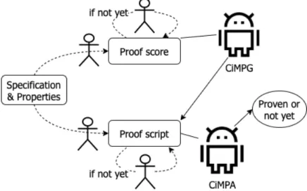
(18) 2.3. CafeInMaude, CiMPA and CiMPG. CafeInMaude [5] is a tool to introduce CafeOBJ [4] specifications into the Maude [6] system. It can be regarded as the second implementation of CafeOBJ in addition to the original one, which was done in Common Lisp. This second implementation has a number of advantages. It improves the performance of some CafeOBJ commands, such as search. It makes CafeOBJ environment easily extensible. That is, it allows us to change the syntax of existing features as well as to introduce new syntax, to add new commands, etc. just by using Maude code, thanks to Maude meta-level features and Full Maude. Using CafeInMaude, we can load the module SIMPLE-NAT in Sect. 2.2 into Maude environment. We can also execute the proof scores with CafeInMaude instead of CafeOBJ to prove the associative property of the plus operator.. Figure 2.1: The relation between proof score, proof script, CiMPA, and CiMPG CafeInMaude is introduced with two extension tools: CiMPA and CiMPG. The former is a proof assistant of CafeInMaude that allows users to write what are called proof scripts to prove invariant properties on their CafeOBJ specifications. The latter is a proof generator of CafeInMaude that provides a minimal set of annotations for identifying proof scores and generating CiMPA scripts for these proof scores. Given a specification in CafeOBJ, to check the satisfiability of some desired properties, users can choose to write proof scripts and executing them with CiMPA. If CiMPA finishes successfully, then the properties are proved; otherwise, we need to revise the proof scripts and make the verification attempt again. However, it is often the case that work9.

(19) ing with proof scores is easier and more flexible. Therefore, users can decide to write proof scores, then use CiMPG to generate proof scripts for CiMPA. Note that proof scores are subject to human errors such that users can overlook some cases, leading to incorrect proofs. CiMPA can get rid of this kind of flaw. If CiMPA does not work on the proof scripts successfully, the proof scores have something wrong and we need to revise the proof scores, making our verification attempt again. Figure 2.1 graphically describes the relation between the proof score, proof script, CiMPA, and CiMPG.. 10.

(20) Chapter 3 Formal verification of an abstract version of Anderson protocol This chapter presents three ways to formally verify that an abstract version of Anderson protocol enjoys the mutual exclusion property. We first give the details of the Anderson protocol and its abstract version in Sect. 3.1 and Sect. 3.2, respectively. Sect. 3.3 describes how to fomally specify the protocol in CafeOBJ. Then, three last sections present three ways of formal verification.. 3.1. Anderson protocol. Anderson protocol [8] is a mutual exclusion protocol. The protocol uses a finite Boolean array whose size is the same as the number of processes participating in the protocol. It also uses the modulo operation of natural numbers and an atomic operation fetch&incmod. fetch&incmod takes a natural number variable x and a non-zero natural number constant N and atomically does the following: setting x to (x+1) % N, where % is the modulo operation, and returning the old value of x. Suppose that there are N processes participating in the protocol. The pseudo-code of Anderson protocol for each process p can be written as follows: Loop “Remainder Section” rs : place[p] := fetch&incmod(next, N ); ws : repeat until array[place[p]]; “Critical Section” cs : array[place[p]], array[(place[p] + 1) % N ] := false, true; 11.

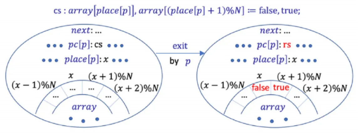
(21) Suppose that each process is located at rs, ws or cs and initially located at rs. place is an array whose size is N and each of whose elements stores one from {0, 1, . . . , N − 1}. Initially, each element of place can be any from {0, 1, . . . , N − 1} but is 0 in this thesis. Although place is an array, each process p only uses place[p], and then we can regard place[p] as a local variable to each process p. array is a Boolean array whose size is N . Initially, array[0] is true and array[j] is false for any j ∈ {1, . . . , N − 1}. next is a natural number variable and initially set to 0. fetch&incmod(next, N ) atomically does the following: setting next to (next + 1) % N and returning the old value of next. x, y := e1 , e2 is a concurrent assignment that is processed as follows: calculating e1 and e2 independently and setting x and y to their values, respectively.. Figure 3.1: The change of state of Anderson when a process p moves to rs from cs Fig. 3.1 graphically visualizes the change of state when a process p moves to rs from cs. The state, which is represented by the right circle, is the successor state of the one which is represented by the left circle. Note that we use pc[p] to denote the location of process p. The changes are highlighted by red color. Since array in Anderson is finite, in the figure, we use a circle (precisely half of a circle) to represent it.. 3.2. A-Anderson protocol. It is challenging to formally verify that Anderson protocol enjoys desired properties, such as the mutual exclusion property, in a sense of theorem proving. This is because the protocol uses a finite array and the modulo operation of natural numbers. Briefly, these reasons make it so difficult for 12.

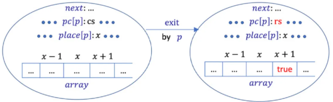
(22) us to conjecture some good lemmas to complete the proof. Then, we make an abstract version of the protocol, which is called A-Anderson protocol. In A-Anderson, we use an infinite Boolean array instead of a finite one, fetch&inc instead of fetch&incmod, and no longer use the modulo operation. The assumption that there are N process participating in the protocol is also removed now. It means that the number of process participating in A-Anderson can be infinite. The pseudo-code of A-Anderson protocol for each process p can be written as follows: Loop “Remainder Section” rs : place[p] := fetch&inc(next); ws : repeat until array[place[p]]; “Critical Section” cs : array[place[p] + 1] := true; where fetch&inc is an atomic operation, taking only one parameter next, and atomically does the following: setting next to next + 1 and returning the old value of next. We also suppose that each process is located at rs, ws or cs and initially located at rs. Initially, each element of place can be any natural number but is 0 in this thesis, array[0] is true, array[j] is false for any non-zero natural number j and next is 0.. Figure 3.2: The change of state of A-Anderson when a process p moves to rs from cs Fig. 3.2 graphically visualizes the change of state when a process p moves to rs from cs. The state, which is represented by the right circle, is the successor state of the one which is represented by the left circle. Let us repeat again that we use pc[p] to denote the location of process p and red color is 13.

(23) used to indicate the changes. Since array in A-Anderson now becomes an infinite array, we represent it in the straight form with infinity on the right side.. 3.3. Specification of A-Anderson protocol in CafeOBJ. In order to specify A-Anderson protocol in CafeOBJ, we first need to define the module LABEL. This module is in charge of defining process locations, i.e., rs, ws and cs. The definition starts with mod! to indicate that it has tight (initial) semantics. This module defines the sort Label and declares three constructors (denoted by the constr attribute): rs, ws, cs. It also defines three equations for the equality predicate to indicate that each label is not equal to any others. mod! LABEL { [Label] ops rs ws cs eq (rs = ws) eq (rs = cs) eq (ws = cs) }. : = = =. -> Label {constr} . false . false . false .. The module SIMPLE-NAT below is in charge of defining natural numbers. In contrast to the module LABEL, this module is defined with keyword mod*, which indicates that it has loose semantics. It first introduces three sorts SZero, SNzNat and SNat represent zero, non-zero numbers and numbers (either zero or non-zero), respectively. The operation s is in charge of defining the successor function of a number, that is it takes a natural number as the input and returns a non-zero number (successor of a natural number n is n + 1). The first three equations define some inequalities. For instance, the first equation says that zero is different from any non-zero number. Then, SIMPLE-NAT declares a predicate “<” that is in charge of defining less-than comparison between two natural numbers. For example, the first equation following the predicate declaration indicates that any natural number is not less than zero. mod* SIMPLE-NAT { [ SZero SNzNat < SNat ] op 0 : -> SZero {constr} 14.

(24) op s : SNat -> SNzNat {constr} vars I J L : SNat vars K G H : SNzNat eq (0 = K) = false . eq (0 = s(I)) = false . eq (I = s(I)) = false . pred _<_ : SNat SNat . eq (I < 0) = false . eq (0 < K) = true . eq (I < s(I)) = true . eq (I < s(s(I))) = true . eq (I < I) = false . ceq (I < s(J)) = true if I < J . ceq (s(I) < J) = false if (I < J) = false . eq (s(I) = s(J)) = (I = J) . ceq (I < s(0)) = false if (I = 0) = false . ceq (I < s(J)) = false if (I = J) = false and (I < J) = false . ceq (s(I) < s(J)) = true if I < J . ceq (I = J) = true if ((I < J) = false and (J < I) = false) . } Then, the module ANDERSON specifies the behavior of the protocol as an OTS SADS . It first imports two modules LABEL, SIMPLE-NAT, and defines the sorts Sys and Pid representing the set of reachable states and the set of process identifiers, respectively as follows: mod* ANDERSON { pr(LABEL + SIMPLE-NAT) [Sys] [Pid] Each state of A-Anderson protocol can be characterized by the following pieces of information: the location of each process, the value stored in next, the value stored in each element of place and the value stored in each element of array. Therefore, we use the following observation functions: op op op op. pc : Sys Pid -> Label . next : Sys -> SNat . place : Sys Pid -> SNat . array : Sys SNat -> Bool .. where Bool is the sort of Boolean values. We do not use any infinite arrays in the specification. Instead, we use the observation function array to observe the value stored in each element that is given to array as its second argument. A constructor is used to represent an arbitrary initial state as follows: 15.

(25) op init : -> Sys {constr} . init is defined in terms of equations, specifying the values observed by the four observation functions in an arbitrary initial state as follows: eq eq eq eq. pc(init,P) = rs . next(init) = 0 . place(init,P) = 0 . array(init,I) = (if I = 0 then true else false fi) .. where P is a CafeOBJ variable of Pid and I is a CafeOBJ variable of SNat. We use three transition functions that are also constructors: op want : Sys Pid -> Sys {constr} op try : Sys Pid -> Sys {constr} op exit : Sys Pid -> Sys {constr} The three transition functions capture the actions that each process moves to ws from rs, tries to move to cs from ws and moves back to rs from cs, respectively. The reachable states are composed of the four constructors. Each of the three transition functions is defined in terms of equations, specifying how the values observed by the four observation functions change. Let S be a CafeOBJ variable of Sys, P & Q be CafeOBJ variables of Pid and I & J be CafeOBJ variables of SNat. want is defined as follows: ceq pc(want(S,P),Q) = (if P = Q then ws else pc(S,Q) fi) if c-want(S,P) . ceq place(want(S,P),Q) = (if P = Q then next(S) else place(S,Q) fi) if c-want(S,P) . ceq next(want(S,P)) = s(next(S)) if c-want(S,P) . eq array(want(S,P),I) = array(S,I) . ceq want(S,P) = S if c-want(S,P) = false . where c-want(S,P) is pc(S,P) = rs. s of s(next(S)) is the successor function of natural numbers. The equations say that if c-want(S,P) is true, the location of P changes to ws, the location of each other process Q does not change, the P’s place changes to next, each other process Q’s place does not change, next is incremented and array does not change in the state denoted want(S,P); if c-want(S,P) is false, nothing changes. try is defined as follows:. 16.

(26) ceq pc(try(S,P),Q) = (if P = Q then cs else pc(S,Q) fi) if c-try(S,P) . eq place(try(S,P),Q) = place(S,Q) . eq array(try(S,P)) = array(S) . eq next(try(S,P),I) = next(S) . ceq try(S,P) = S if c-try(S,P) = false . where c-try(S,P) is pc(S,P) = ws and array(S,place(S,P)) = true The equations say that if c-try(S,P) is true, the location of P changes to ws, the location of each other process Q does not change, place does not change, array does not change and next does not change in the state denoted try(S,P); if c-try(S,P) is false, nothing changes. exit is defined as follows: ceq pc(exit(S,P),Q) = (if P = Q then rs else pc(S,Q) fi) if c-exit(S,P) . eq place(exit(S,P),Q) = place(S,Q) . eq next(exit(S,P)) = next(S) . ceq array(exit(S,P),I) = (if I = s(place(S,P)) then true else array(S,I) fi) if c-exit(S,P) . ceq exit(S,P) = S if c-exit(S,P) = false . } where c-exit(S,P) is pc(S,P) = cs. The equations say that if c-exit(S,P) is true, the location of P changes to rs, the location of each other process Q does not change, place does not change, next does not change, the Ith element of array is set true if I equals s(place(S,P)) and each other element of array does not change in the state denoted exit(S,P); if c-exit(S,P) is false, nothing changes.. 3.4 3.4.1. Formal verification with proof scores The mutual exclusion property. One desired property A-Anderson protocol should satisfy is the mutual exclusion property. To specify the property, the following module ADS-INV is introduced:. 17.

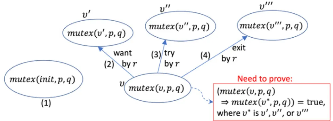
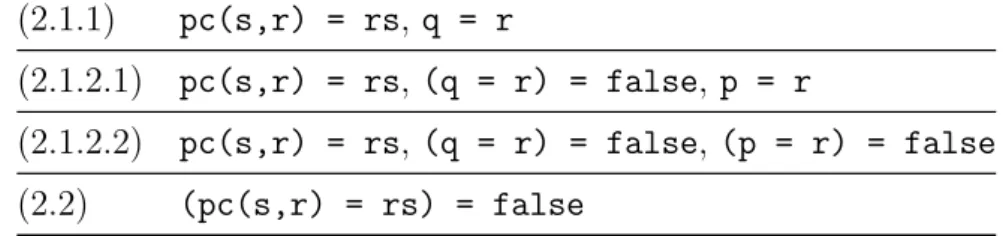
(27) mod ADS-INV { pr(ANDERSON) var S : Sys . vars P Q : Pid . vars G H : SNzNat . vars I J K : SNat . op mutex : Sys Pid Pid -> Bool eq mutex(S,P,Q) = ((pc(S,P) = cs and pc(S,Q) = cs) implies (P = Q)) . } The mutual exclusion property is formalized as the following invariant wrt SADS : (∀υ ∈ RSADS )(∀p, q ∈ Pid) mutex(υ, p, q). Let us use “the proof of mutex wrt SADS ” (and “to prove mutex wrt SADS ”) to mean the proof of (∀υ ∈ RSADS )(∀p, q ∈ Pid) mutex(υ, p, q) (and to prove (∀υ ∈ RSADS )(∀p, q ∈ Pid) mutex(υ, p, q)). This calling is applied for not only SADS or mutex, but also other OTSs as well as other similar CafeOBJ operators invi that takes one state variable and zero or more data values and returns a Boolean value in this thesis. We may omit “wrt S” if S is clear from the context. Note that, initially, ADS-INV only has mutex that is used to formalized the mutual exclusion property, but while conducting the formal verification, we gradually conjecture lemmas and add them to ADS-INV on the fly.. Figure 3.3: The proof of mutex wrt SADS The proof of mutex wrt SADS is essentially done by applying structural induction on the state variable. The approach is graphically depicted in Fig. 3.3. There are four cases to tackle: base case (1) and three induction cases (2), (3), (4). In (1), we need to show that mutex holds in any initial states. In (2), (3) and (4), we want to prove that if mutex holds in state υ, it 18.

(28) Table 3.1: Case splittings for case (2) in the proof of mutex wrt SADS (2.1.1). pc(s,r) = rs, q = r. (2.1.2.1) pc(s,r) = rs, (q = r) = false, p = r (2.1.2.2) pc(s,r) = rs, (q = r) = false, (p = r) = false (2.2). (pc(s,r) = rs) = false. also holds in the successor states υ 0 , υ 00 and υ 000 of υ, where υ 0 , υ 00 and υ 000 are made by transitions when an arbitrary process r moves to ws from rs, tries to move to cs from ws and moves to rs from cs, respectively. Firstly, the proof score of the base case (1) init is as follows: open ADS-INV . ops p q : -> Pid . red mutex(init,p,q) . close Feeding the proof score into CafeInMaude, CafeInMaude returns true meaning that the case is discharged. Next, let us consider case (2). What to prove is mutex(want(s,r),p,q), where s is a fresh constant of Sys representing an arbitrary state and p, q & r are fresh constants of Pid representing arbitrary process IDs. The induction hypothesis is mutex(s,P,Q) for all process IDs P & Q. Let us note that s is shared by mutex(want(s,r),p,q) and mutex(s,P,Q), while the variables P and Q can be replaced with any terms of Pid, such as p and q. Unlike the base case (1), case (2) can not be discharged directly, instead, it requires us to conduct case splitting. We first split case (2) into two subcases: (2.1) pc(s,r) = rs and (2.2) (pc(s,r) = rs) = false. Case (2.2) can be discharged, its proof score is as follows: open ADS-INV . op s : -> Sys . ops p q r : -> Pid . eq (pc(s,r) = rs) = false . red mutex(s,p,q) implies mutex(want(s,r),p,q) . close Feeding the proof score into CafeInMaude, true is returned. Case (2.1) needs to be split into two sub-cases: (2.1.1) q = r and (2.1.2) (q = r) = false. Case (2.1.1) can be discharged, while we need to split case (2.1.2) into two sub-cases one more time: (2.1.2.1) p = r and (2.1.2.2) 19.

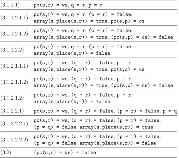
(29) Table 3.2: Case splittings for case (3) in the proof of mutex wrt SADS (3.1.1.1). pc(s,r) = ws, q = r, p = r. (3.1.1.2.1.1). pc(s,r) = ws, q = r, (p = r) = false, array(s,place(s,r)) = true, pc(s,p) = cs. (3.1.1.2.1.2). pc(s,r) = ws, q = r, (p = r) = false, array(s,place(s,r)) = true, (pc(s,p) = cs) = false. (3.1.1.2.2). pc(s,r) = ws, q = r, (p = r) = false, array(s,place(s,r)) = false. (3.1.2.1.1.1). pc(s,r) = ws, (q = r) = false, p = r, array(s,place(s,r)) = true, pc(s,q) = cs. (3.1.2.1.1.2). pc(s,r) = ws, (q = r) = false, p = r, array(s,place(s,r)) = true, (pc(s,q) = cs) = false. (3.1.2.1.2). pc(s,r) = ws, (q = r) = false, p = r, array(s,place(s,r)) = false. (3.1.2.2.1). pc(s,r) = ws, (q = r) = false, (p = r) = false, p = q. (3.1.2.2.2.1). pc(s,r) = ws, (q = r) = false, (p = r) = false, (p = q) = false, array(s,place(s,r)) = true. (3.1.2.2.2.2). pc(s,r) = ws, (q = r) = false, (p = r) = false, (p = q) = false, array(s,place(s,r)) = false. (3.2). (pc(s,r) = ws) = false. (p = r) = false. Both sub-cases now can be discharged. The case splittings for case (2) also can be seen through Table 3.1. So far, we have completely resolved two cases (1) and (2) in the proof of mutex wrt SADS . These are two simple cases since case (1) is discharged directly and case (2) is discharged just after three times of case spitting without using any other invariants as lemmas. Unfortunately, it is not simple likewise to discharged case (3). In case (3), we need to prove mutex(try(s,r),p,q), where s is a fresh constant of Sys and p, q & r are fresh constants of Pid. Table 3.2 shows the case splittings for case (3) in the proof of mutex wrt SADS . For example, the open-close fragment of case (3.1.1.2.1.1) is as follows: open ADS-INV . op s : -> Sys . ops p q r : -> Pid . eq pc(s,r) = ws . 20.

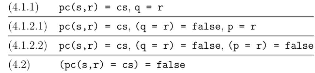
(30) eq q = r . eq (p = r) = false . eq array(s,place(s,r)) = true . eq pc(s,p) = cs . red mutex(s,p,q) implies mutex(try(s,r),p,q) . close Feeding the fragment into CafeInMaude, CafeInMaude returns false. Case (3.1.1.2.1.1) says that process p is located at cs, process r (or q since q = r) is located at ws and array(s,place(s,r)) is true. In that case, process r can move to cs, breaking the property concerned since there are two processes p and r located at cs. Therefore, we need to conjecture a lemma to discharge case (3.1.1.2.1.1). Such a lemma can be conjectured from the assumptions made in case (3.1.1.2.1.1). We have conjectured inv1 as such a lemma. inv1 is declared in the module ADS-INV as follows: eq inv1(S,P,Q) = ((array(S,place(S,P)) = true and pc(S,P) = ws and (P = Q) = false) implies (pc(S,Q) = cs or (pc(S,Q) = ws and array(S,place(S,Q)) = true)) = false) . where S is a CafeOBJ variable of Sys, P and Q are CafeOBJ variables of Pid. The red command in the above open-close fragment now becomes as follows: red inv1(s,r,p) implies mutex(s,p,q) implies mutex(try(s,r),p,q) . CafeInMaude now returns true for the proof score fragment. The proof of case (3.1.2.1.1.1) needs the use of inv1(s,r,q) as a lemma. The remaining sub-cases of case (3) (in Table 3.2) can be discharged without any lemmas. Table 3.3: Case splittings for case (4) in the proof of mutex wrt SADS (4.1.1). pc(s,r) = cs, q = r. (4.1.2.1) pc(s,r) = cs, (q = r) = false, p = r (4.1.2.2) pc(s,r) = cs, (q = r) = false, (p = r) = false (4.2). (pc(s,r) = cs) = false. Case (4) can be discharged likewise by applying case splittings as shown in Table 3.3. Let us repeat again that s is a fresh constant of Sys, while p, q & r are fresh contants of Pid, and in (4) we need to prove mutex(exit(s,r),p,q). All of the sub-cases can be discharged straightforwardly, without any lemmas. 21.

(31) 3.4.2. The other lemmas. Since the proof of mutex uses inv1 as a lemma, we need to prove that inv1 is also an invariant wrt SADS to complete the formal verification. The proof of inv1 requires four other invariants that are inv2, inv3, mutex and inv6. The proof of inv3 uses another invariant inv4 as a lemma. The proof of inv4 uses another invariant inv5 as a lemma. inv2 and inv5 can be proved independently without the use of any other lemmas. The proof of inv6 uses inv1, inv4, mutex and inv7 as lemmas. The proof of inv7 uses inv2, inv6 and inv8 as lemmas. The proof of inv8 uses inv2 as a lemma. These invariants are declared in the module ADS-INV as follows: eq inv2(S,P) = ((pc(S,P) = cs) implies (array(S,place(S,P)) = true)) . eq inv3(S,P,Q) = ((place(S,P) = place(S,Q) and (P = Q) = false) implies (place(S,P) = 0)) . eq inv4(S,P) = (place(S,P) = next(S) implies (next(S) = 0)) . eq inv5(S,P) = (place(S,P) < s(next(S))) = true . eq inv6(S,P) = ((pc(S,P) = ws and array(S,place(S,P)) = true) or pc(S,P) = cs) implies array(S,next(S)) = false . eq inv7(S) = array(S,s(next(S))) = false . eq inv8(S,I,J) = (array(S,J) = true and I < s(J)) implies array(S,I) = true . where s in s(next(S)) and s(J) is the successor function of natural numbers. Let us note that although the proof of mutex uses inv1 as a lemma and the proof of inv1 uses mutex as a lemma, our argument is not circular. We use simultaneous induction to conduct our proof. The correctness of this method has been formally proved in the papers [2, 3]. To prove each invariant for an OTS by writing proof scores, we first use simultaneous induction on states and do the following: for the base case, it is usually straightforward to discharge the case, and for each induction case, we conduct case splittings and use instances of induction hypotheses (or lemmas) as premises of implications. It took much less than 1s to run all proof scores with CafeInMaude so as to formally verify that A-Anderson protocol enjoys the mutual exclusion property. The experiment used a computer that carried 3.4GHz microprocessor and 32GB main memory. The same computer was used to conduct the other experiments mentioned in the thesis. 22.

(32) 3.5. Formal verification with CiMPA. We have presented in the previous section the proof score approach proving that A-Anderson protocol enjoys the mutual exclusion property. The proof score approach is flexible in a sense of theorem proving. The approach, however, has a disadvantage. Proof scores are subjected to human errors. From the previous section, it can be seen that humans can overlook some cases, but they are not pointed out. Using CiMPA can help us get out of this disadvantage. The proof score approach to formal verification does not require to explicitly construct proof trees. The outcomes of the approach are open-close fragments that correspond to leaf parts of proof trees. Conducing formal verification by writing proof scores, however, we implicitly construct proof trees. Once we have completed formal verification by writing proof scores and executing them with CafeInMaude, we must be able to conduct the formal verification with CiMPA. We partially describe the formal verification with CiMPA that A-Anderson enjoys the mutual exclusion property. We first introduce the goals to prove for CiMPA with the command :goal as follows: open ADS-INV . :goal{ eq [inv1 :nonexec] : inv1(S:Sys,P:Pid,Q:Pid) = true . eq [inv2 :nonexec] : inv2(S:Sys,P:Pid) = true . eq [inv3 :nonexec] : inv3(S:Sys,P:Pid,Q:Pid) = true . eq [inv4 :nonexec] : inv4(S:Sys,P:Pid) = true . eq [inv5 :nonexec] : inv5(S:Sys,P:Pid) = true . eq [inv6 :nonexec] : inv6(S:Sys,P:Pid) = true . eq [inv7 :nonexec] : inv7(S:Sys) = true . eq [inv8 :nonexec] : inv8(S:Sys,I:SNat,J:SNat) = true . eq [mutex :nonexec] : mutex(S:Sys,P:Pid,Q:Pid) = true . } where :nonexec instructs CafeInMaude not to use the equations as rewrite rules. Then, we select S with the command :ind on as the variable on which we start proving the goals by simultaneous induction: :ind on (S:Sys) :apply(si) where si stands for simultaneous induction. The command :apply(si) starts the proof by applying simultaneous induction on S, generating four 23.

(33) Table 3.4: Sub-goals of 3-9 3-9-1-1-1 csb3_9_1, csb3_9_2, csb3_9_3 3-9-1-1-2. csb3_9_1, csb3_9_2, ¬csb3_9_3. 3-9-1-2. csb3_9_1, ¬csb3_9_2. 3-9-2. ¬csb3_9_1. Table 3.5: Sub-goals of 3-9-1-1-2 3-9-1-1-2-1-1 csb3_9_4, csb3_9_5 3-9-1-1-2-1-2. csb3_9_4, ¬csb3_9_5. 3-9-1-1-2-2. ¬csb3_9_4. sub-goals: 1, 2, 3 and 4 corresponding to exit, init, try and want. Note that, the order between four sub-goals is different from that in the proof score approach since CiMPA generates them in alphabetical order. Each sub-goals consists of nine equations to prove, corresponding to inv1, ..., mutex. We skip the sequence of commands that discharge the first two sub-goals for exit and init. We partially describe how to discharge the third sub-goal for try. To this end, the first command used is as follows: :apply(tc) where tc stands for theorem of constants. The command generates nine sub-goals as follows: 3-1. > TC eq [inv1 :nonexec]: inv1(try(S#Sys,P#Pid),P@Pid,Q@Pid) = true . ... 3-9. TC eq [mutex :nonexec]: mutex(try(S#Sys,P#Pid),P@Pid,Q@Pid) = true . where seven more equations should be written in the place ..., the > symbol indicates that this is the current goal. The command :apply(tc) replaces CafeInMaude variables with fresh constants in goals. S#Sys and P#Pid are fresh constants introduced by :apply(si), while P@Pid and Q@Pid are fresh constants introduced by :apply(tc). Let us consider goal 3-9, to discharge goal 3-9, we first use the following commands: 24.

(34) :def csb3_9_1 = :ctf {eq pc(S#Sys,P#Pid) = ws .} :apply(csb3_9_1) :def csb3_9_2 = :ctf {eq Q@Pid = P#Pid .} :apply(csb3_9_2) :def csb3_9_3 = :ctf {eq P@Pid = P#Pid .} :apply(csb3_9_3) Based on the three equations, four sub-goals are generated as in Table 3.4. In the table, we use the names of equations (where based on them we apply case splitting) such as csb3_9_1, csb3_9_2 to express for the corresponding equation holds. For example, csb3_9_1 expresses for pc(S#Sys,P#Pid) = ws, and ¬csb3_9_1 expresses for (pc(S#Sys,P#Pid) = ws) = false. For sub-goal 3-9-1-1-1 (three equations hold), we use the following commands: :imp [mutex] by {P:Pid <- P@Pid ; Q:Pid <- Q@Pid ;} :apply (rd) The induction hypothesis is instantiated by replacing the variables P:Pid and Q:Pid with the fresh constants P@Pid and Q@Pid and the instance is used as the premise of the implication. Then, :apply(rd) is used to check if the current goal can be discharged. The goal is discharged in this case. The goal corresponds to case (3.1.1.1) in the previous section. The current goal is now switched to 3-9-1-1-2. We then use the following commands: :def csb3_9_4 = :ctf [ array(S#Sys,place(S#Sys,P#Pid)) .] :apply(csb3_9_4) :def csb3_9_5 = :ctf {eq pc(S#Sys,P@Pid) = cs .} :apply(csb3_9_5) Based on one Boolean term and one equation, three sub-goals are generated as in Table 3.5. In the table, we use csb3_9_4 to express for array(S#Sys, place(S#Sys,P#Pid)) = true, and ¬csb3_9_4 to express for array(S#Sys, place(S#Sys,P#Pid)) = false. For sub-goal 3-9-1-1-2-1-1 (the Boolean term is true and the equation holds), we use the following commands: :imp [inv1] by {P:Pid <- P#Pid ; Q:Pid <- P@Pid ;} :imp [mutex] by {P:Pid <- P@Pid ; Q:Pid <- Q@Pid ;} :apply (rd). 25.

(35) The lemma inv1 is instantiated by replacing the variables P:Pid and Q:Pid with the fresh constants P#Pid and P@Pid, respectively, then the instance is used as a part of the premise of the implication. Next, the induction hypothesis is instantiated by replacing the variables P:Pid and Q:Pid with the fresh constants P@Pid and Q@Pid, respectively, and the instance is also used as a part of the premise of the implication. After that, :apply(rd) is introduced to check if the current goal can be discharged. The goal is discharged in this case. The goal corresponds to case (3.1.1.2.1.1) in the proof score approach presented in Sect. 3.4. The remaining goals can be resolved likewise. When CiMPA is used to formally verify invariant properties for an OTS, what to do is essentially the same as we do formal verification by writing proof scores. The difference is, obviously, we need to use the commands given by CiMPA when conducting formal verification with CiMPA. It took about 22s to run the proof scripts with CiMPA so as to formally verify that A-Anderson protocol enjoys the mutual exclusion property.. 3.6. Formal Verification with CiMPG. After writing proof scores to prove that A-Anderson protocol enjoys the mutual exclusion property, we can confirm that the proof scores are correct by doing the formal verification with CiMPA as described in the last section. Although we are able to conduct the formal verification with CiMPA once we have completed formal verification by writing proof scores, it would be preferable to automatically confirm the correctness of proof scores. CiMPG makes it possible to automatically confirm the correctness of proof scores by generating proof scripts for CiMPA from the proof scores. To use CiMPG, we need to add one more open-close fragment to the proof scores. The open-close fragment is as follows: open ADS-INV . :proof(ander) close where ander is just an identifier, can be replaced by another one that is more preferred. Furthermore, we need to add :id(ander) in each open-close fragment. For example, the open-close fragment of case (3.1.1.2.1.1) introduced in Sect. 3.4 becomes as follows:. 26.

(36) open ADS-INV . :id(ander) op s : -> Sys . ops p q r : -> Pid . eq pc(s, r) = ws . eq q = r . eq (p = r) = false . eq array(s,place(s,r)) = true . eq pc(s,p) = cs . red inv1(s,r,p) implies mutex(s, p, q) implies mutex(try(s, r), p, q) . close Feeding the annotated proof scores into CiMPG, CiMPG generates the proof scripts for CiMPA. The generated proof scripts are quite similar to the one written manually. Feeding the generated proof scripts into CiMPA, CiMPA discharges all goals, confirming that the proof scores are correct. In A-Anderson case study, CiMPG took about 626s to generate the proof scripts from the correct proof scores. This chapter has presented three ways of formal verification that AAnderson protocol enjoys the mutual exclusion property. Each of the three verification techniques has advantages as well as disadvantages, but by conducting formal verification in three ways, we triple-check the correctness of our proof. We can summarize what has been presented in this chapter as well as some lessons learned from the case study as follows: • Once we have completely conducted formal verification by writing proof scores, it is rather straightforward to develop the verification with proof scripts and CiMPA. • Although CiMPG can automatically generate the proof scripts for CiMPA from proof scores, it takes time to do so. However, in the case study, 10 minutes waiting is still acceptable, at least in comparison with writing proof scripts manually. • Abstraction makes it possible to achieve formal verification. Three verification techniques helped us complete the formal verification of A-Anderson, but could not achieve the same result with Anderson. However, we have successfully used “simulation-based verification for invariant properties [10]” so as to formally verify that Anderson enjoys the mutual exclusion property even though this part is not presented in this thesis.. 27.

(37) • Auxiliary lemmas are required in all three ways of formal verification. Lemma conjecture is the most intellectual task while conducting formal verification of A-Anderson. In the upcoming chapter, a lemma conjecture technique will be introduced.. 28.

(38) Chapter 4 Formal verification of MCS protocol This chapter describes how to formally verify that MCS protocol enjoys the mutual exclusion property. We first present a lemma conjecture technique called Lemma Weakening (LW). Then, the usefulness of this technique is demonstrated along with the formal verification of MCS.. 4.1. Lemma Strengthening (LS) and Lemma Weakening (LW). Suppose that we want to prove that a state predicate p is an invariant wrt an OTS S. It is often the case that p is not inductive and then there is a transition instance that does not preserve p such that p(υ) holds but p(υ 0 ) does not, where υ → υ 0 is a transition instance, which is shown in Fig. 4.1 (a), where ∆p is {υ ∈ Υ | p(υ)}. This is the reason why invariant proofs become non-trivial or even can become very hard. If we can successfully show that the source υ is not reachable wrt S, then we do not need to consider the transition instance, being able to discharge the case. One possible way to do so is to find pstr that is stronger than p such that pstr (υ) does not hold and to prove that pstr is an invariant wrt S, which is shown in Fig. 4.1 (b). If pstr is inductive wrt S, we do not need to use any more lemmas. This approach has been summarized as the proof rule Inv by Manna and Pnueli [11]. To prove that p is an invariant of S (or a state machine), in general, we need to find an inductive invariant q wrt S such that q(υ) ⇒ p(υ) for all states υ ∈ Υ. In practice, q is often in the form p ∧ p0 , and p0 is often in the form q1 ∧ . . . ∧ qn . q1 , . . . , qn are the lemmas of the proof that p is an invariant wrt S. It is often the case that we do not know any of q1 , . . . , qn 29.

(39) Figure 4.1: The reason why invariant proofs become non-trivial and two approaches to tackling the non-trivial situation in advance. We need to gradually conjecture q1 , . . . , qn one by one when we encounter the situation shown in Fig. 4.1 (a). For example, in the previous Chapter, to prove that mutex is an invariant wrt SADS , it requires to use inv1 as a lemma, and during the proof of inv1, we conjecture some more other lemmas. mutex corresponds to p, while mutex ∧ inv1 ∧ . . . ∧ inv8 corresponds to the inductive invariant q. qi (υ) for the source υ needs not to hold but does not need to be properly stronger than p because p ∧ q1 ∧ . . . ∧ qn is surely stronger than p. In general, when we have conjectured up to qk , we do not know how many more lemmas we need to conjecture. The reason why invariant proofs become non-trivial or even can become very hard is because there exists a transition instance υ → υ 0 as shown in Fig. 4.1 (a). The proof rule Inv gets rid of such a transition instance as shown in Fig. 4.1 (b). Another possible way to get rid of such a transition instance is to find pwk that is weaker than p such that pwk (υ 0 ) holds and to prove that pwk is an invariant wrt S, which is shown in Fig. 4.1 (c). Even though pwk is an invariant wrt S, however, it does not guarantee that p is an invariant wrt S. This is because ∆p may not contain all reachable states in RS . Therefore, the second approach is not used to prove that p is an invariant wrt S. This might be the reason why the second approach has been rarely used. Although the second approach is not very useful for p, it may be useful for some qi , a lemma of the proof that p is an invariant wrt S. In this thesis, strengthening lemmas qi is called Lemma Strengthening (LS), while weakening lemmas qi is called Lemma Weakening (LW). While proving that MCS enjoys the mutual exclusion property, we have encountered a situation where use of only LS did not seem to make the proof converge. We got over the situation by using LW to weaken some lemmas. Note that we have used both LS and LW for the proof that MCS enjoys the mutual exclusion property. We will describe in which way LW makes the 30.

(40) proof attempt converge in Sect. 4.4. Two upcoming sections describe MCS and formal specification of SMCS that formalizes the protocol.. 4.2. MCS list-based queuing lock protocol. MCS is a mutual exclusion protocol invented by Mellor-Crummey and Scott [1]. Variants of MCS have been used in Java VMs and therefore the 2006 Edsger W. Dijkstra Prize in Distributed Computing went to their paper [1]. This protocol has the following properties: • it guarantees FIFO ordering of lock acquisitions; • it spins on locally-accessible flag variable only; • it requires a small constant amount of space per lock; and • it works equally well (requiring only O(1) network transactions per lock acquisiion) on machines with and without coherent caches. The pseudo-code of MCS protocol for each process p can be written as follows: rs : l1 : l2 : l3 : l4 : l5 : l6 : cs : l7 : l8 : l9 : l10 : l11 : l12 :. “Remainder Section” nextp := nop; predep := fetch&store(glock , p); if predep 6= nop { lockp := true; nextpredep := p; repeat while lockp ; } “Critical Section” if nextp = nop { if comp&swap(glock , p, nop) goto rs; repeat while nextp = nop; } locknextp := false; goto rs;. There is one global variable glock shared by all processes participating in MCS protocol. Its value is a process ID (Pid) or nop, a dummy process ID. glock basically refers to the bottom element if the queue is not empty. Each process p maintains three local variables nextp , lockp and predep whose types are Pid, Bool and Pid, respectively. Initially, glock, nextp , lockp and predep are nop, nop, false and nop, respectively. nextp and predep are used to construct a global queue of processes (or process IDs). Basically, nextp 31.

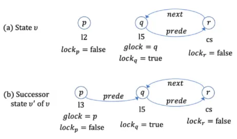
(41) Figure 4.2: The change of state of MCS when a process p moves to l3 from l2 refers to the next element of the queue if p is in the queue. Note that nextp may be nop even though p is not the bottom element of the queue. predep refers to the predecessor element of the queue. lockp is the local lock on which process p is spinning while lockp is true to wait for entering the critical section. MCS uses two non-trivial atomic instructions: fetch&store and comp&swap. For a variable x and a value α, fetch&store(x, α) atomically does the following: x is set to α and the old value of x is returned. For a variable x and values α, β, comp&swap(x, α, β) atomically does the following: if x equals α, then x is set to β and true is returned; otherwise false is just returned. Fig. 4.2 graphically visualizes the change of state of MCS when a process p moves to l3 from l2. In the state υ, which is represented by Fig. 4.2 (a), processes p, q, and r, located at l2, l5, and cs, respectively; glock is q; next of r is q; and prede of q is r. When process p moves to l3, glock is set to itself, and its prede is set to q (depicted in Fig. 4.2 (b)).. 4.3. Specification of MCS protocol in CafeOBJ. In order to specify MCS protocol in CafeOBJ, we first need to define the module LABEL, which is in charge of defining process locations. This module first introduces the sort Label and declares fourteen constructors (denoted by the constr attribute): rs, l1, l2, l3, l4, l5, l6, cs, l7, l8, l9, l10, l11. 32.

(42) and l12. It also defines many equations for the equality predicate to indicate that each label is not equal to any others. mod! LABEL { [Label] ops l1 l2 l3 l4 l5 l6 l7 l8 l9 l10 l11 l12 rs cs : -> Label {constr} . eq (l1 = l2) = false . eq (l1 = l3) = false . ... eq (l1 = rs) = false . eq (l1 = cs) = false . eq (l2 = l3) = false . eq (l2 = l4) = false . ... eq (l2 = cs) = false . eq (l3 = l4) = false . ... eq (l12 = cs) = false . eq (rs = cs) = false . }. where many other equations should be written in the place ..., constr indicates that rs, l1, l2,..., l12 are constructors of sort Label. The module PID is in charge of defining process identifiers. Sort Pid represents the (correct) process identifiers, while sort Nop expresses for the erroneous identifiers which are the dummy processes. Sort Pid&Nop is a supersort of sorts Pid and Nop. The module also states that any correct identifier is different from nop. mod* PID { [Nop Pid < Pid&Nop] op nop : -> Nop {constr} . var P : Pid . eq (P = nop) = false . }. Finally, the module MCS specifies the behavior of the protocol as an OTS SMCS . It first imports two modules LABEL, PID, and defines the sort Sys representing the set of reachable states as follows: mod* MCS { pr(LABEL + PID) [Sys]. Each state of MCS protocol can be characterized by the following pieces of information: the value of glock; the location, next process, previous process, lock value of each process. Therefore, the following observation functions are used: 33.

(43) op op op op op. glock : Sys -> Pid&Nop . pc : Sys Pid -> Label . next : Sys Pid -> Pid&Nop . prede : Sys Pid -> Pid&Nop . lock : Sys Pid -> Bool .. since the values of glock, next_p, prede_p can be nop, thus we need to use sort Pid&Nop instead of sort Pid. Then, a constructor is used to represent an arbitrary initial state as follows: op init : -> Sys {constr} .. init is defined in terms of equations, specifying the values observed by the five observation functions in an arbitrary initial state as follows: eq eq eq eq eq. glock(init) = nop . pc(init,P) = rs . next(init,P) = nop . prede(init,P) = nop . lock(init,P) = false .. where P is a CafeOBJ variable of Pid. Fourteen following functions specify the transitions of MCS: -op -op -op -op -op -op -op -op -op -op. moves want moves stnxt moves stprd moves chprd moves stlck moves stnpr tries chlck moves exit moves chnxt moves chglk. to l1 from rs : Sys Pid -> Sys {constr} to l2 from l1 : Sys Pid -> Sys {constr} to l3 from l2 : Sys Pid -> Sys {constr} to l4 or cs from l3 : Sys Pid -> Sys {constr} to l5 from l4 : Sys Pid -> Sys {constr} to l6 from l5 : Sys Pid -> Sys {constr} to move to cs from l6 : Sys Pid -> Sys {constr} to l7 from cs : Sys Pid -> Sys {constr} to l8 or l11 from l7 : Sys Pid -> Sys {constr} to l9 or l10 from l8 : Sys Pid -> Sys {constr}. 34. . . . . . . . . . ..

(44) -op -op -op -op. moves to go2rs : tries to chnxt2 : moves to stlnx : moves to go2rs2 :. rs from l9 Sys Pid -> Sys {constr} move to l11 from l10 Sys Pid -> Sys {constr} l12 from l11 Sys Pid -> Sys {constr} rs from l12 Sys Pid -> Sys {constr}. . . . .. Each of the above fourteen functions is followed by a comment line that describes the corresponding transition of a process it captured. For example, if a process p is located at l1 in state s, then stnxt(s, p) denotes the state just after p has executed the statement at l1 and moves to l2 from l1. The reachable states are composed of these fourteen transition functions plus init function. Each of the fourteen transition functions is defined in terms of equations, specifying how the values observed by the five observation functions change. Let S be a CafeOBJ variable of Sys, P & Q be CafeOBJ variables of Pid. want transition is defined as follows: eq glock(want(S,P)) = glock(S) . ceq pc(want(S,P),Q) = (if P = Q then l1 else pc(S,Q) fi) if pc(S,P) = rs . eq next(want(S,P),Q) = next(S,Q) . eq lock(want(S,P),Q) = lock(S,Q) . eq prede(want(S,P),Q) = prede(S,Q) . ceq want(S,P) = S if (pc(S,P) = rs) = false .. the equations say that if the location of process P currently is rs, then P’s location changes to l1, the location of each other process Q does not change; next, lock, prede of every processes and glock do not change. If currently process P is not located at rs, nothing changes. In the same way, chlck transition is defined as follows: eq glock(chlck(S,P)) = glock(S) . ceq pc(chlck(S,P),Q) = (if P = Q then (if lock(S,P) then l6 else cs fi) else pc(S,Q) fi) if pc(S,P) = l6 . eq next(chlck(S,P),Q) = next(S,Q) . eq lock(chlck(S,P),Q) = lock(S,Q) . eq prede(chlck(S,P),Q) = prede(S,Q) . ceq chlck(S,P) = S if (pc(S,P) = l6) = false .. 35.

(45) the equations say that if currently the location of process P is l6 and lock of P is true, then P’s location changes to cs. next, lock, prede of every processes and glock do not change. If currently process P is not located at l6, nothing changes. The remaining transitions can be defined likewise. All of them can be found at the webpage presented in Chapter 1.. 4.4. Formal verification with proof scores. This section presents the proof score approach to formal verification that MCS protocol enjoys the mutual exclusion property. Since the complete proof is quite long, we will only present here a part of it. We will separately describe the use of LS and LW in the verification.. 4.4.1. Use of Lemma Strengthening (LS). Similar to the A-Anderson case study, we introduce the module MCS-INV to specify the mutual exclusion property. The module is as follows: mod MCS-INV { pr(MCS) var S : Sys vars P Q : Pid op mutex : Sys Pid Pid -> Bool eq mutex(S,P,Q) = ((pc(S,P) = cs and pc(S,Q) = cs) implies (P = Q)) . }. The equation mutex says that there is always at most one process located at the critical section at any given time. mutex(S,P,Q) is proved for all reachable states S and all process IDs P & Q by structural induction on S. There are fifteen cases to tackle including: (1) init, (2) want, (3) stnxt, (4) stprd, (5) chprd, (6) stlck, (7) stnpr, (8) chlck, (9) exit, (10) chnxt, (11) chglk, (12) go2rs, (13) chnxt2, (14) stlnx, (15) go2rs2. Similar to the A-Anderson case study, the base case (1) init can be discharged straightforwardly. Considering case (2), we need to prove mutex(want(s,r),p,q), where s is a fresh constant of Sys representing an arbitrary state and p, q and r are fresh constants of Pid representing arbitrary process IDs. The induction hypothesis is mutex(s,P,Q) for all process IDs P & Q. Let us repeat again that s is shared by mutex(want(s,r),p,q) and mutex(s,P,Q), while the variables P and Q can be replaced with any 36.

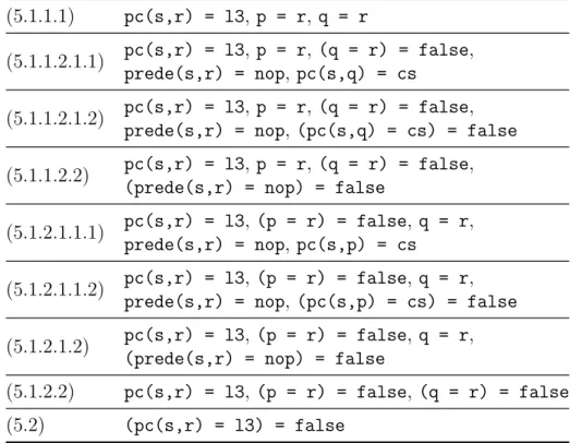
(46) Table 4.1: Case splittings for case (2) in the proof of mutex wrt SMCS (2.1.1). pc(s,r) = rs, q = r. (2.1.2.1) pc(s,r) = rs, (q = r) = false, p = r (2.1.2.2) pc(s,r) = rs, (q = r) = false, (p = r) = false (2.2). (pc(s,r) = rs) = false. terms of Pid, such as p and q. Case (2) is discharged by splitting it into four sub-cases as shown in Table 4.1. It is not always straightforward likewise to discharged the thirteen remaining cases. We are required either to split cases much more times or to conjecture new lemma to discharge a case. The former creates a huge number of open-close fragments as well as lines of code. The latter is always considered as one of the most challenging tasks in theorem proving. Next, let us consider case (5) as the evidence for this argument. Table 4.2: Case splittings for case (5) in the proof of mutex wrt SMCS (5.1.1.1). pc(s,r) = l3, p = r, q = r. (5.1.1.2.1.1). pc(s,r) = l3, p = r, (q = r) = false, prede(s,r) = nop, pc(s,q) = cs. (5.1.1.2.1.2). pc(s,r) = l3, p = r, (q = r) = false, prede(s,r) = nop, (pc(s,q) = cs) = false. (5.1.1.2.2). pc(s,r) = l3, p = r, (q = r) = false, (prede(s,r) = nop) = false. (5.1.2.1.1.1). pc(s,r) = l3, (p = r) = false, q = r, prede(s,r) = nop, pc(s,p) = cs. (5.1.2.1.1.2). pc(s,r) = l3, (p = r) = false, q = r, prede(s,r) = nop, (pc(s,p) = cs) = false. (5.1.2.1.2). pc(s,r) = l3, (p = r) = false, q = r, (prede(s,r) = nop) = false. (5.1.2.2). pc(s,r) = l3, (p = r) = false, (q = r) = false. (5.2). (pc(s,r) = l3) = false. In case (5), what we need to prove is mutex(chprd(s,r),p,q), where s is a fresh constant of Sys and p, q & r are fresh contants of Pid. Table 4.2 shows 37.

(47) the case splittings for case (5). Let us consider sub-case (5.1.1.2.1.1). In (5.1.1.2.1.1), mutex(s,p,q) reduces to true, whille mutex(chprd(s,r),p,q) reduces to false, and then mutex(s,p,q) implies mutex(chprd(s,r),p,q) reduces to false. The pair of states s and chprd(s,r) is a transition instance as shown in Fig. 4.1 (a). We need to conjecture and use a lemma to discharge (5.1.1.2.1.1). One possible lemma conjectured most straightforwardly can be constructed by combining the equations that characterize (5.1.1.2.1.1) with conjunction, negating the whole formula and replacing the fresh constants s, p, q & r with variables S, P, Q & R [12]. Since the formula constructed is in the form (not P = R) or F that is equivalent to (P = R) implies F . Thus, the lemma constructed is F in which R is replaced with P , which is equivalent to the following: eq inv1’(S,P,Q) = ((pc(S,P) = l3 and prede(S,P) = nop and (P = Q) = false) implies (pc(S,Q) = cs) = false) .. Since inv1’(s,p,q) reduces to false, we can use inv1’ as a lemma to discharge (5.1.1.2.1.1) as follows: red inv1’(s,p,q) implies mutex(s,p,q) implies mutex(chprd(s,r),p,q) .. In the proof of inv1’, however, we encounter a sub-case (1’.8.1.1.2.2.1.1) in which CafeInMaude returns false for its proof score. The open-close fragment is as follows: open MCS-INV . op s : -> Sys . ops p q r : -> Pid . eq pc(s,r) = l6 . eq p = r . eq (q = r) = false . eq lock(s,r) = false . eq pc(s,q) = l3 . eq prede(s,q) = nop . red inv1’(s,p,q) implies inv1’(chlck(s,r),p,q) . close. By applying the same technique that has been explained above to conjecture inv1’, we can conjecture another lemma to discharge (1’.8.1.1.2.2.1.1) as follows: eq inv1’’(S,P,Q) = ((pc(S,Q) = l3 and prede(S,Q) = nop and (P = Q) = false) implies (pc(S,P) = l6 and lock(S,P) = false) = false) .. 38.

(48) The conditional part of inv1’’ is exactly the same as that of inv1’. The reason why we use the forms of inv1’ and inv1’’ is because we emphasize what are shared by inv1’ and inv1’’. The proof of inv1’’ needs yet another lemma whose conditional part is exactly the same as that of inv1’. We need several different lemmas when we only use the most straightforward lemmas. Therefore, we strengthen them to obtain the following lemma: eq inv1(S,P,Q) = ((pc(S,Q) = l3 and prede(S,Q) = nop and (P = Q) = false) implies ((pc(S,P) = cs or pc(S,P) = l7 or pc(S,P) = l8 or pc(S,P) = l10 or pc(S,P) = l11 or (pc(S,P) = l6 and lock(S,P) = false)) = false)) .. And the red command in the open-close fragment of case (5.1.1.2.1.1) now becomes as follows: red inv1(s,p,q) implies mutex(s,p,q) implies mutex(chprd(s,r),p,q) .. The proof of inv1 needs totally less lemmas than that of inv1’. More precisely, the set of lemmas that need to be used in the proof of inv1 is a subset of those in the proof of inv1’. Table 4.3: Case splittings for case (8) in the proof of mutex wrt SMCS (8.1.1.1). pc(s,r) = l6, p = r, q = r. (8.1.1.2.1). pc(s,r) = l6, p = r, (q = r) = false, lock(s,r) = true. (8.1.1.2.2.1). pc(s,r) = l6, p = r, (q = r) = false, lock(s,r) = false, pc(s,q) = cs. (8.1.1.2.2.2). pc(s,r) = l6, p = r, (q = r) = false, lock(s,r) = false, (pc(s,q) = cs) = false. (8.1.2.1.1). pc(s,r) = l6, (p = r) = false, q = r, lock(s,r) = true. (8.1.2.1.2.1). pc(s,r) = l6, (p = r) = false, q = r, lock(s,r) = false, pc(s,q) = cs. (8.1.2.1.2.2). pc(s,r) = l6, (p = r) = false, q = r, lock(s,r) = false, (pc(s,q) = cs) = false. (8.1.2.2). pc(s,r) = l6, (p = r) = false, (q = r) = false. (8.2). (pc(s,r) = l6) = false. The proof of case (8) also requires another lemma. Table 4.3 shows the case splittings for case (8). Let us repeat again that s is a fresh constant 39.