JAIST Repository: Generalized kernel canonical correlation analysis : criteria and low rank kernel learning

Japan Advanced Institute of Science and Technology

JAIST Repository

https://dspace.jaist.ac.jp/

Title Generalized kernel canonical correlation analysis : criteria and low rank kernel learning

Author(s) Nguyen, Canh Hao; Ho, Tu Bao; Renders, Jean-Michel; Cancedda, Nicola

Citation

Research report (School of Knowledge Science, Japan Advanced Institute of Science and Technology), KS-RR-2009-002: 1-21 Issue Date 2009-02-20

Type Technical Report

Text version publisher

URL http://hdl.handle.net/10119/8449

Rights

Description リサーチレポート（北陸先端科学技術大学院大学知識

Genera踊zedKernelCanonicalCorrelationAna【ysis= CriteriaandLowRankKernelLearning CanhHaoNguyen,TuBaoHo,Jean-MEChelRenders andNico[aCancedda February20,2009 KS-RR-2009-002

Generalized

Kernel Canonica

Criteria

and Low Rank

1 Correlation

Analy

Kernel Learning

sis:

Canh Hao Nguyen, Tu Bao Ho, Jean-Michel Renders and Nicola Cancedda

Email: [email protected]

School of Knowledge Science

Japan Advanced Institute of Science and Technology

JAIST Research Report: KS-RR-2009-002 February 22, 2009

Abstract

Canonical Correlation Analysis is a classical data analysis technique for computing common correlated subspaces for two datasets. Recent advances in machine learning enable the technique to operate solely on kernel matrices, making it a kernel method with the advantages of modularity, efficiency and nonlinearity. Its performance is also improved with appropriate regularization and low-rank approximation methods, making it applicable to many practical applications.

However, the classical technique is applicable to find correlation of only two datasets. It is a practical problem that we wish to consider correlation of more than two datasets at the same time. Such problems occurs in many domains such as multilingual text processing, where we wish to find a common represen-tation of parallel document corpora from more than two languages altogether

(we call this situation multiple view or multiview for short). Generalizing CCA to more than two views face some problems, namely: finding criteria for multi-view CCA and available computational solutions for these criteria.

In this report, we analyze the criteria that have been proposed to be ob-jective functions for multi-view CCA. We obtain that only some of them are suitable for our purpose. In these criteria, only one of them, namely MAX-VAR, has an efficient solution. We describe our algorithm for this criterion. We conduct experiments on a multi-lingual corpora. Experiment results show

that multi-view CCA brings an advantage over two view CCA when there are not too many training data are available.

We then show that low rank approximation of kernels are done indepen-dently from views. This could be a disadvantage as different views may be projected onto subspaces that may not result in correlation. We then propose a new incomplete Cholesky decomposition procedure that simultaneously de-composes all views. Experiment results show that the new ICD, by making sure the alignment of subspaces from different views, give a higher performance for multiview CCA when there are many views and a few dimensions for ap-proximation.

1 Introduction

Introduction: Canonical Correlation Analysis (CCA) is a statistical method to find linear correlation between two (or more) multidimensional variables. It was proposed by H. Hotelling [9]. CCA can be kernelized, therefore it inherits all advantages of kernel methods [14], namely computational efficiency, modularity and nonlinearity.

The starting idea of CCA is that we may receive different views, or different data rep-resentations of inherently the same objects. In biological samples express differently

in different biological experiments [17, 5] . The same documents are translated into different languages [12]. From multiple views to the same object, one wishes to find a common, latent semantic representation of the object itself. This may seem to be impossible as it is task-dependent. However, the good news is that in that common semantic representation, the object is uniquely represented. This leads to the fact that there exist transformations from different views into the common semantic space that should result in the common representation. To this end, it is the purpose of CCA to enforce the correlation of different views after being transformed into the common semantic space.

Background: CCA is the problem of finding each basic vectors sets, one for each

set of (multidimensional) variables, such that the correlation between the projections

of these variables onto their corresponding basics are maximized. We describe only the first basic vectors for each set for now.

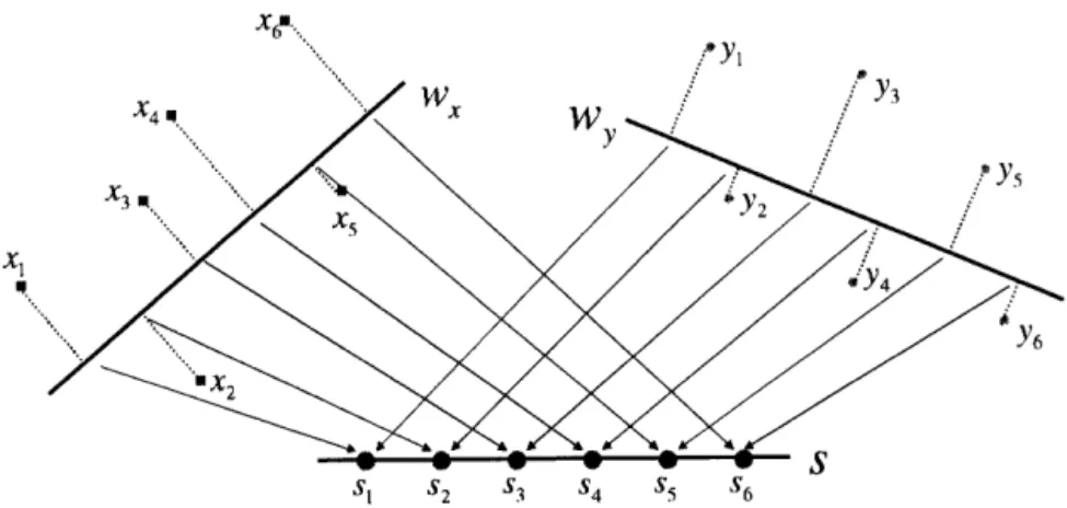
Given X = {x1, x2 • • • x,,,} and Y = {yl, y2 • • • yn} where xi E Rn' and yi E Rn2, the problem is to find wx E Rill and wy E Rn2 so that the projections of X onto wx and Y onto wy are maximized. Without loss of generality, we assume that E 1 xi = 0 and Eni=1 yi = 0.

Projection on wx: xi --> (xi, wy), therefore the projections of X become {wx X }T = XT wx (X is considered as a column vector). Similarly, projections of Y onto wy are YT wy. The objective of CCA is to maximize the correlation with respect to wx and

x1 I X4 X3 X6111.._. x5 wx Wy Y, Y2 Y3 Y4 Y5 R Y6 • x2 S Si S2 S3 S4 S5 S6

Figure 1: Canonical Correlation Analysis: projecting two sets of data onto subspaces that are maximally correlated.

p= max corr(XT wx, YT w) = max

wz,wyWs,wy (XT wx, YT wy) p = max wx,w6, IIXTwxII . IIYTwyI wx X YT wy wT X X T wX.wT YYT wy

Denote: CCx = X XT , Cyy = YYT (these are correlation matrices), Cyx = YXT (cross-correlation matrices).

T

p = max

_wx,wy

l/wxxxwx

. wy

cyywy

(1)

(2)

Cxy = XYT and

(3)

Here, p is called canonical correlation and wx, wy are called canonical variates or canonical variables. A pictorial description of the algorithm is shown in figure 1. In this paper, we first describe the CCA algorithm in the next section, followed by its kernelization, regularization and low rank versions using Incomplete Cholesky Decomposition for computational efficiency. We then analyze its multiple views gen-eralization criteria to see which ones are suitable and solvable for very large scale applications. We describe the formulations for the criteria and show their interpreta-tions. Experiments are presented to show that advantage of multiview version when there are a few training data points. We when propose a new ICD algorithm that simultaneously decompose kernel matrices from different views, which is supposed to preserve more correlation so that the multiview CCA would have a higher

perfor-mance.

2 Canonical Correlation Analysis

Formula 1 is equivalent to maximizing its numerator subject to the following con-straints: wI CCxwx = 1 and wT Cyywy = 1.

Lagrangian is

L(A, Ay,

wx,

wy)

=wTCyywy—Ax

(wxCCxwx—1)—Ay(wyCyywy

—

1). (4)

Taking derivatives in respect to wx and wy give us: Cyywy—AxCxxwx=0(5)

Cy,w, — AyCyywy = 0•(6) Taking the constraints into account, we have A = Ay = A. The solution:Assuming Cyy is invertible.

CyyCyXWX

wy=---A(7)

CyyCCXw~

--- ACxxwx

—

0•(8)

Cyy

CyXWX

= A2C„w,(9)

Therefore, the solution to the problem can be calculated using an inversion of a matrix 7 and a generalized eigenvalue problem 9.

Note 1: Equations 5 and 6 can be rewritten as:

0 CyywX _{_ A CCx 0 wx(10)}

Cyx 0wy0 Cyy wy

(CxxCxy(Wx(l+A)(Cxx

0

wx(11)

Cyx Cyy wy0 Cyy wy

2.1 Kernelization

Above is the linear version of CCA where we need to find canonical covariates that after linear projections, views are correlated. However, the class of linear functions is not able to capture nonlinear relations among views, which is the case in practice. For that reason, one needs to use a larger class of functions. It is usually the case

that one settles to the space called Reproducing Kernel Hilbert Space [15], which is large enough to capture nonlinear relation and small enough not to contain many non-smooth functions. The space is defined to be any combination of kernel function k (being a positive semidefinite function):

f(.) _ aik(•, x). (12)

By the virtue of the Representer theorem [16], we know that in this particular case, canonical covariates have its representation (for both X and Y):

wx

= Eaik(•,xi), xi E X.

Having known that wx lies in the span of columns of X and wy lies in the span of columns of Y, we may rewrite the equation 3 using wx = Xa and wy = Y/3, where aERn and ,3eRn:

aT XT • XYT • Ya

p max_{, ,/(aTXT • XXT • Xa) • (,3TYT • YYT • Ya)} (14)

p = max a,Q

aT KxKy,d

given that KK = XT X and Ky = YT Y. Again, Lagrangian is:

aT K2a . /3T2/3

(15)

L(Aa,A

,a,,(3)

=aTKxKyi3—

Aa(aTK~a—

1) —2~(,3TKy,3—

1)

2

(16)

In a similar fashion as before, taking derivatives in respect to a and ,3, we have Aa=Aa=Aand

KX

Ky,d

—

AKK

a = 0

KyKXa—AKK/3=0

The solution: When Ky is invertible then:

K-'K~a

,Q= yA(19)

and

KKKKa = A2KKKKa(20)

This means that perfect correlation (A = 1) can be obtained with any a. We have the problem of overfitting here.

Note 2: Equations 17 and 18 can be rewritten as:

0 KxKy a KxKx 0 a(21)A

Ky KX 0 ,Q0 KyKy ,Q

KXKX KxKy a _{= (1 + A) KxKx 0a (22)}

KyKX KyKy,Q0KyKy,Q

We arrive at one generalized eigenvalue problem (of the 2n * 2n matrix) .

Note 3: Since the solution can be computed using kernel matrices KK and Ky, nonlinear transformation of original variables can be introduced into this problem in

a similar fashion as other kernel methods.

2.2 Regularization

As mention before, the cases, in which perfect correlation and any a can be a canonical covariate, would happen. Therefore, regularization is necessary to avoid nonsense

solution (overfitting). It is introduced as follows:

p= max _a7 aT K~Ky~ (23)

V (aTicza+kI wxl 2) . (13TKy/3"+ IIwyII2)

aT KxKy/

p=max

_{a,Q /(aTKa + kaT}

_{Kxa) . (13T}

K2/3

+ k/3TK

13)

Lagrangian is:

L(A ,A ,a,13)

= aTKxKy,Q—

a2a(aTK2a+kaTKxa-1)—a213(13TKyfi+k13TKy13-1)

Taking derivatives, proving as = )Q = A, we arrive at:

KXKy/3 — A(KX + kI)KKa = 0,"(26) KyKKa—A(Ky+kI)Ky,Q=0.(27)

The solution: If Ky is invertible, we have:

(Ky + kI)-1KXa(28)

A and substituting into 26 give us:

KXKy(Ky + kI)-1KKa = A2KX(KX + kI)-1a(29)

This give us the generalized eigenvalue problem. When KC is also invertible, we have:

(KC + kI)-1Ky(Ky + kI)-1KKa = A2a(30)

Note 4: Equations 26 and 27 can be rewritten as:

0

KXKya

(KK

+ kI)KK

0a

(31)

Ky

K,

0Q0

(Ky + kI) Ky,Q

(KK

+ kI) KK

KKKya

= (1+~)(KK+ kI) KK

0

KyKK

(Ky + kI )Ky0

(Ky + kI )Ky

(32)

Note 5: In Bach & Jordan, (KC

+ kI)KK is approximated

with (KC

+ 2I)2, arriving

at:

(Kr + k J)2

KKKa(Kr+t_020a

KyKK (Ky

+ZI)2

—

(1+A) 0(Ky + ZI)2

(33)

2.3 Efficient Computation

To reduce the computation load, it is better to approximate the kernel matrices with lower rank ones. The reasons are:

• Efficient matrix inversion and eigen-decomposition, making these methods ear in n - number of data objects, as opposed to n3 originally.

7

• It is observed that many kernel matrices have low ranks. Advantages have

already been taken for SVMs [4] .

• It is natural to expect much linear dependency among variables in the same sets

when working with CCA (if they are independent, overfitting may happen and meaningless correlations occur). Therefore, the kernel matrix is likely to be of

low rank.

An efficient approximation is Incomplete Cholesky decomposition [6] or its dual imple-mentation Gram-Schmidt orthogonalization. In the end, we will have lower rank ap-proximations of kernel matrices as: KK = RXRTx and Ky = RyRT , where Rx E Rn*ml and Ry E Rn*m2. Both Rx and 14 are lower triangular matrices and ml, m2 << n. In the reduced dimensional space, d = Rx cx E Rml and ,C3 = RT 13 E Rm2. Plugging

into formulas 26 and 27, we have:

Putting RTx an

RX

Rx

Ry

Ry

,Q

—

ARX

(RTx

RX

+ kI) Rx a = 0

RyRTR,Rxa

—

ARy(RTRy

+ kI)RT13

= 0

d Ry into the left hand side of the above

equations

gives

us:

RT

RX

RT

Ry

Ry

,Q

—

ART

RX

(Rx

RX

+ kI) Rx cx

= 0

RTRyRTRXRTcx

—

ARTRy(RTRy

+ kI)Ry,Q

= 0

(34) (35) (36) (37) Let ZXX Zyy Zxy Zyx = Rx Rx e Rml*ml, = RT RyERm2*m2 , = RT Ry E Rml*m2 = RT RXERm2*m1• ₍₃₈₎ We have finally:

ZXXZXy,Q — AZXX(ZXX + kI)d = 0 ZyyZyXE — AZyy (Zyy + kI)13 = 0 Assuming (again) that ZZx and Zyy are invertible, then:

Zxy—A(Zxx+kI)d=0 Zyxa—A(Zyy+kI)13=0 (39) (40) (41) (42)

The solution: _ (Zyy + kI)-1 Zyxa To compute composition SyE Rm2 *m2 Zyx ( Zyy A

+ kI)-1Zyxii = A2(ZZx + kI)a (ZZx + kI)-1 and (Zyy + kI)-1 efficiently, do , (ZZx + kI) = SXST and (Zyy + kI) = SyST

are lower triangular matrices.

a complete where SS E Cholesky Rm1*M1 (43) (44) de-and Note 6: S; 1 Zxy The formulas 41 (sT)-1S-1Z

1~.7yyyx (SD-1a = A2a.

and 42 can be rewritten in a matrix form:

(45) 0 Zyx Zxy 0 a _(ZZx+kI) 0 0 (Zyy + kI ) a 13 (46) (ZZx+kI) Zyx Zxy (Zyy + kI) a (1 + A) (ZZx + kI) 0 0 (Zyy + kI)

We then arrive at a generalized eigenvalue problem of a matrix with size Once a and ,Q are computed, original solution can be recovered as:

a

13)

•

So far, we are dealing with correlation of two sets of variables. This section describe how to deal with m sets of variabels, called m views. here we first analyze criteria to generalize CCA to m views. We then describe MAXVAR, the criterion with known efficient solutions.

In practice, it is anticipated that sometimes data express in more than two views. It is the case of documents are translated in many languages. An example is Acquis, the European constitutional body. Each document are translated into 23 languages. Of course, taking into account two views would be a solution. However, having only two views may bring more canonical covariates than it should, spurious correlations may

happen. Having additional views would give a more reliable estimations of correlation among view, making the set of canonical covariates smaller. By having a smaller set of canonical covariates, with the assumption that all semantic representations arc

x, x4111_. x31 x6 ^ x5 wx Wy Y1 Y2 w Y3 Y4 Y5 Y6 x2 s, s2 S3 s4 s5 S ZIA Z3 _Z4 1 Z2 A 6 wz 1 Zs

Figure 2: Generalizing CCA into multiview: projecting data from different views into a common subspace S, where semantically equivalent data points arc projected into an unique point.

captured by those covariates, we expect to have a more concise (smaller and more reliable) representation of semantics. A pictorial description of multiview CCA is

shown in figure 3

The central problem for generalizing CCA into multiview is the objective function of the multiview correlation. As in the classical two-view case, correlation is the objective function. However, correlation is defined for two random variables only. When generalizing into more than two views, there is nothing such as correlation. Here come the problem of defining what is a correlation for multiview version. There are attempts to define correlation for multiview, but one must bear in mind that there are several constraints. First, it must carry the meaning of correlation for our purpose of capturing common semantics of different views. Second, for a practical reason, the computational mean must be available for such objective functions. Here, we mean that there must be a solution to optimize the objective functions that scales well with large or massive data sets.

The next subsection will discuss the proposed criteria and we will analyze to see if they satisfy those constraints.

Criteria SUMCOR MAXVAR SSQCOR MINVAR GENVAR Usage in ML Min-sum-of-distance MKCCA No KerICA KerICA Suitability Yes Yes Yes No No Has solutions No Yes No Yes Yes Table 1: Analysis of CCA generalization criteria.

3.1 Analysis of criteria

For the two view problem

as before,

correlation

is the only objective

function

has

been taken into account

so far. However,

when

having

more than two views,

there

are many

ways

to define

correlation

among

a set of projections

from

different

views.

The objectives

for multiview

CCA

can be analyzed

from

the correlation

matrix

of all

projected

vectors.

Here, we discuss

only the objective

functions

for solving

the first

correlation

variates.

The following

correlation

variates

can be computed

in the same

way,

with an additional

constraint

of orthogonality

of projections.

Fortunately,

this

constraint

is automatically

satisfied

by the solutions.

First is some notations. Suppose

that having

m views,

Xi, X2 ... Xm, which

are

row-wise

centered.

The target is to find m projections

into w1, W2

... w.,,,,

such that

XT

wi are maximally

correlated

(the meanings

of maximally

correlated

are defined

later). Denote:

_{Ci.7 = XiXT}

_{, li = f(wT Ciiwi)}

_{be the length}

_{of the projected}

_vector,

ei =xwiwould be the normalized projected vector. Denote: C is the full covariance matrix comprising of and D is the block-diagonal matrix of Cii. We now have:

= 1 and 1T ei = 0. The correlation matrix of ei is a m * m matrix = {Oij } _1

satisfying:

=< ei, ei > .(49)

There are some works in Statistics that propose criteria for generalizing CCA into

more than m views [13], [10], and [7]. All the criteria basically measure how well projections of views are grouped together in the feature space. Hence, most of them are based on the matrix 43. The criteria proposed in [10] arc milestones. Other works just modify them to incorporate other information such as covariance into the criteria. The list of criteria is in the first column of table 3.1. It is noteworthy that all these criteria are equivalent to each other when m = 2.

The second column shows how these criteria are known and used in the Machine Learning community. We analyze these criteria to see if which ones would be suitable for our purpose, named Suitability in the table 3.1. The last column shows if using

these criteria may give a efficient enough algorithm for large scale application. SUM-COR is known to be the sum of square distance measure. It is the most intuitive criterion without any known efficient solution. In fact, it is equivalent to a multivari-ate eigenvalue problem where there exist no theories to shed a light on its solutions.

It is known to have a very large number of solutions in [3] . MAXVAR is known to be a generalized eigenvalue problem and has been proposed and used in [1, 13, 17].

SSQ-COR has not been used due to the fact that it is not known to be formulated to any easily solvable problem. The two criteria MINVAR and GENVAR are not considered to be suitable for generalized CCA for the following reason. As long as there is any linear dependency among projections of all the views, MINVAR and GENVAR would get the maximum value, indicating a perfect correlations among all projections. In fact, linear dependency does not guarantee perfect correlations for more than two random variables. These criteria are, therefore, used to measure independency in

ICA [1] .

3.2 MAXVAR

We start with another objective function:

m m

p3

= max

E

wT

Cijwj,

i=1 j=1

(50)

subject to: E wT Ciiwi = 1.

Theorem 1: p3 is the maximum generalized eigenvalue (Amax) of the following

gen-eralized eigenvalue problem. C11 C12 • • Clm C21 C22 • • • C2m Cml Cm2 • • Cmm wl W2 turn = A . Diag(C11, C22, .. • Cmm)

Proof: Lagrangian of the objective function:

m m

L(w,

A)

= E >wC3w3

—

A(> wT

Ciiwi

- 1).

Taking derivatives with respect to wi for all is

ECijwj = ^Ciiwi.

j=1

Multiplying wT to the left hand side of each part of 53, we have:

E wT

Cijwj

= AwT

Ciiwi.(54)

j=1 Summing over i from 54 then:

m m

EE wT

Cijwj

= A.(55)

i=1 j=1

We have p3 is an eigenvalue of 51. Now we need to prove it is the largest one.

If p3 = A < Amax then the exists a (normalized) wmax is the generalized eigenvector

corresponding to the eigenvalue Amax. Then:

m m

Amax

= EE Wi

maxCijwj—max

> A = p3-(56)

i=1 j=1

This contradicts the optimality of p3. Hence, p3 = Amax.

Note 7: One can conclude that maximizing p3 is equivalent to finding the maximum eigenvalue of the generalized eigenvalue problem.This is different from the problem in ?? only at having the same A instead of different Ai. The difference between pi and

p3 is the weighting of each (normalized) projected vector ei with its length i . p3 is,

in fact, a weighted version of pi.

Geometrical interpretation of the weights: The weights li are introduced from wi, which are, in turn, introduced by the generalized eigenvalue problem. However, we can get some ideas from equation 54.

Having liei = XTwi, the right hand side of the equation 54 is: AwT Ciiwi = A • l2.

The left hand side is

mmm

E wT

Cijwj

= wT

Xi E WT

xj =< liei,

E13e3

> .

j=1 j=1j=1

Denote le =E jm 1 ljej be the sum of all un-normalized projected vectors, then A•li

liei, le >. li= <ei,e>. A < ei, le > = Ali. (57) (58) =< (59) (60) 13

Hence, the weight of a projected vector ei in the objective function is the dot product between it and the weighted mean.

In light of the correlation matrix 43, we can see that:

/ 011 012 ... Olm11>j _{< el, lie.; >< el, le >11} 021 022 • • • 02m l2 _{_Ej < e2, lie.;>=< e2, le >_12}

\Oml 0m2•• 0mm imE. < em,lie >< em, le >lm ( 61)

Refer to 60 for the last equation.

This means that the weights Ii form a eigenvector for the correlation matrix. This also

means that the objective function p3, equivalently A (see 55), is actually maximizing an eigenvalue of the correlation matrix 4).

Theorem 2: Amax is the maximum eigenvalue of all the correlation matrices obtained from projections of Xi into wi.

Proof: Denote li = 1 XTwi l l , L = I/1,12 _{• • • lm }T , e, =x awti as usual.}

AmaxWTCW ^max— max WTDW `

immT

L_i=1Lj=1wicijwj

= max m

Ei=1wT ciiwi Eim=1~j=1 < liei, ljej >

= maxn+ 2 w~i=1 li Eim—i1lilj< ei,ej> = max~m_ wLm _{i=1 li} 2 T = maxL(1)L(62) w LT L •

One can observe that we can scale wi independently of other wj, therefore li can receive any value independently of other l j . As W runs all over its space, L also runs all over its space.

Therefore, LT (13LA max = max --- w LT L T = maxL(DI, L LTL•

Then, Amax is also the maximum eigenvalue of all eigenvalues of all correlation

ma-trices. This means that p3 is the MAXVAR criterion in [10].

3.2.1 Kernelization and Regularization

In a similar fashion as [1], we can come to the kernelized form of the objective as

finding the maximal eigenvalue of:

K1K1 K1K2 • • • KiKm alal K2 K1 K2K2 ... K2Km a2a2

. = A•Diag(KiK1, K2K2, ... KmKm) . KmKi KmK2 • • • KmKmam"

(64)

If we regularize like PLS wT w, then the above problem becomes:

0 K1 K2 ... KiKmal1 K2 K1 0 • • • K2Km a2

•

KmK1 KmK2 ... 0am/

(al)

= A • Diag(K1K1 + kK1i K2K2 + kK2, . . . KmKm + kK,,)a2.(65)

am

If we want to regularize futher aT a, the it becomes: 0 K1 K2 ... KiKmal K2 K1 0 ... K2Km a2 KmK1KmK2 • .. 0 am a1 a2 =A•Diag(K1K1+kI,K2K2+kI,... KmKm +kI)(66) am/ 3.2.2 Efficient Computation

For the PLS regularization, proceeding similarly as in section 5 or previous subsection, we arrive at the reduced dimensional form:

0 Z12 ••• Zim Z21 0 •.. Z2m Zml Zm2 •.• 0 al a2 am _ A•Diag(Z11+kI,Z22+kI,... Zmm+kI) al a2 am (67)

If the aTa regularization then:

0 Z12 ••• Zlm Z21 0 ... Z2m Zml Zm2 - .. 0 al a2 am = ,\•Diag(Z11+kZ111, Z22+kZ21, ... Zmm+kZmm) al a2 am (68)

Original solution can be recovered by:

ai = K22 l l ~i ai = UiAZV , Kii1=UZAI2Ui,

wi = XiUiAi lUai. (69)

4 Algorithm and Experiments

4.1 Algorithm

The algorithm we implemented is using MAXVAR criterion, which is known to be the generalized eigenvalue problem. There are two part of the algorithms: learning, i.e. determining the canonical covariate and testing, i.e. projecting test data into the common subspace. Learning part follows strictly the description in section 2.3 and

3.2. The the generalized eigenvalue problem, we use the BLOPEX package [11] . There are two ways for the testing part. One is to go from di to ai and wi, then testing data is projected into these canonical covariate directly. Another way, as described in [8], is to project the data into the low dimensional space and perform projections there. We found that the second way is not only much more efficient, but also give much more stable results. Unstability and inefficiency come from the fact that in the former way, one needs to pseudo-inverse the reduced dimensional kernel matrices. Matrix pseudo-inversion is very expensive and unstable.

We has tried and found that the implementation is scalable so far for 30000 training

data for 4 languages (totalling 120000 training data points).

4.2 Experiments

We would like to evaluate this algorithm to see whether having more than two views can be beneficial for some cross language information retrieval tasks. We choose the Mate Retrieval task in our experiments. The data is the alignments of the JRC-Acquis Corpus 1. It contains alignment of sentences from pair languages. As we

need a multiple view corpus, we merged from different pairs together to create on multiple alignment corpus. About merging alignment pairs, about 90% are retained after merging. Any conflict in merging is discarded.

The experiments were setup as follows. The baseline is the two language case, en and fr, and multiple view version is four languages: de, en, fr, and es. We trained models for the two and four view settings. In the testing face, we query in en and expect the answer in fr in both cases. Euclidean distance is used to retrieve mates. We used two measures for the result, top 1% retrieval and average mate rank. Training data were randomly sampled from the corpus. The sizes of training data were 50, 100, 200, 500, 1000, 2000 and 5000. For each size, we sampled 5 training data sets. For testing, we sampled 10 testing sets of size 1000.

Parameters of the experiments were set as follows. We used linear kernel. The maximum dimension of the low dimensional approximation was 300. Regularization

with k were set as recommended in [1] . For the generalized eigenvalue problem, we

run the 4000 iterations. We extracted 30 eigenvalue-eigenvector pairs. Results are depicted in the figure 4.2. On the horizontal axes are the sizes of training sets. The vertical axes are the measures with respect to different training sizes. Any point in

the graphs is the average of 50 measures from 5 models on 10 data sets.

The conclusion we derived from this graph is that having four views does not improve the retrieval rates when the training sizes are 500 or more. The two view version is more tailored to the language pair. The multi-view version is beneficial when there are few training data. The reason is that in that case, two view version is not relible enough and additional data helps. When there are more data, the two view version is more tailored to the task.

5

Low Rank Kernel

Learning

Suppose that views lie in spaces R1 R2, • • • Rm. We wish to find for each view a subspace Ri C Ri so that after projecting data onto these subspaces, data from

ihttp://www .jrc.it/langtech

90 88 86 84 82 80 78 76 Top 1% Retrieval $• P P P •• •. 2 languages + w 4 languages 50 100 200 500 1000 2000 5000 32 30 28 26 24 22 20 18 16 14

Average Mate Rank

z q i • • • 2 languages + — 4 languages •ViV 50 100 200 500 1000 2000 5000

Figure 3: Retrieval results of different sizes of the set.

different views become correlated.

However, using original spaces RZ to discover RZ is, being a generalized eigenvalue problem with MAXVAR as analyzed in the previous section, is computationally ex-pensive for moderate sizes. One usually use some efficient approximation. As for mKCCA, in the kernel setting, the usual technique is using low rank approximation of kernel matrices to have efficient training.

Customizing Incomplete Cholesky Decomposition for CCA. The problem is that not the same semantic space from different views are attracted as ICD is carried out independently from each view. We found that in the 5000 sizes data sets, for the two view version, about 80% of the data objects are in common when ICD picks them for the spanning set of the low dimensional space. For four-view version, the number drops to about 64%. In order to ensure that the same semantic space are extracted from different languages, one needs to have a customized ICD for this purpose. This

resembles the work in [2], and indeed is mentioned as a future work.

5.1 Incomplete Cholesky Decomposition with side tion

Our idea is to use ICD that makes sure that 100% of data picked are in common. This can be done by simultaneously decomposing all data matrices at the same time. The data object picked by by ICD each time is common among all views; the one which overall reduces the most the trace of the projected data matrices is picked.

5.2 Experiments

As before, we train on 5 data samples of different sizes (from 50 to 5000). The models are then used to test on 10 samples of size 1000. The figure shows an average of 50 results, which are the success rates of retrieving the right mate within the top 1%. mKCCA setting is as the previous section, with the low rank approximation of kernel matrices of 50 (set fixed on these experiments).

It shows that for two-view version, the new ICD algorithm gives a some performance improvement. However, on the four-view version, the improvements are seen more clearly. The reason could be the fact that the four-view version has less data points in common.

6 Conclusion and Future Works

The contributions of this paper are: an overall analysis of criteria for generalizing CCA into multiple views and a new ICD algorithm specially for generalized CCA. We showed that the MAXVAR, as proposed and used by others are the only crite-rion with known efficient solution. We provided an implementation. On the dataset we evaluated on, the multiple view versions show to improve performances of Mate Retrieval tasks when there are few training data. The new ICD algorithm we pro-posed simultaneously decompose kernels from different views to make sure that they retain more correlation on the projected subspaces. Experiments show that new ICD algorithm gives generalized CCA a higher performance.

References

[1] Francis R. Bach and Michael I. Jordan. Kernel independent component analysis.

Journal of Machine Learning Research, 3:1-48, 2003.

[2] Francis R. Bach and Michael I. Jordan. Predictive low-rank decomposition for kernel methods. In ICML '05: Proceedings of the 22nd international conference

on Machine learning, pages 33-40, New York, NY, USA, 2005. ACM Press. [3] Moody T. Chu and J. Loren Watterson. On a multivariate eigenvalue

lem, part is algebraic theory and a power method. SIAM Journal on Scientific

Computing, 14(5):1089-1106, 1993.

[4] Shai Fine and Katya Scheinberg. Efficient svm training using low-rank kernel

representations. Journal Machine Learning Research, 2:243-264, 2002.

[5] Bernd Fischer, Volker Roth, and Joachim M. Buhmann. Time-series alignment

by non-negative multiple generalized canonical correlation analysis. BMC forrnatics, to appear.

2 view version 86 84 82 80 78 76 74 72 70 .^• —Old ICD ---I-41-- new ICD

50 100 200 500 1000 2000 5000 4 view version d m 0, u 84 82 80 78 76 re74 72 70 50 100 200 500 1000 Data size 2000 5000

Figure 4: Comparing the original and new ICD algorithms for mKCCA. New ICD algorithm gives mKCCA a higher performance, especially when there are more views and smaller rank is used to approximate kernels.

[6] Gene H. Golub and Charles F. Van Loan. Studies in Mathematical Sciences). The Jo

1996.

Matrix Computations (Johns Hopkins

has Hopkins University Press, October

[7] Mohamed Hanafi and Henk A. L. Kiers. Analysis of k sets of data, with

tial emphasis on agreement between and within sets. Computational Statstistics

and Data Analysis, 51(3):1491-1508, 2006.

[8] David R. Hardoon, Sandor R. Szedmak, and John R. Shawe-Taylor. Canonical

correlation analysis: An overview with application to learning methods. Neural

Computation, 16(12):2639-2664, 2004.

[9] Harold Hotelling. Relations between two sets of variables. Biometrika,

372, 1936.

[10] Jon R. Kettenring. Canonical analysis of sevaral sets of variables. Biometrika,

58:433-451, 1971.

[11] A. V. Knyazev, M. E. Argentati, I. Lashuk, and E. E. Ovtchinnikov. Block locally optimal preconditioned eigenvalue xolvers (blopex) in hypre and petsc.

IAM Journal on Scientific Computing (SISC), to appear.

[12] Yaoyong Li and John Shawe-Taylor. Using kcca for japanese-english language information retrieval and document classification. Journal of Intelligent

Information Systems, 27(2):117-133, 2006.

[13] George Michailidis and Jan de Leeuw. The gifi system for descriptive multivariate analysis. Statistical Science, 1998.

[14] John Shawe-Taylor and Nello Cristianini. Kernel Methods for Pattern Analysis. Cambridge University Press, New York, NY, USA, 2004.

. [15] Vladimir N. Vapnik. Statistical Learning Theory. Wiley-Interscience, September

1998.

[16] Grace Wahba. Spline models for observational data. SIAM [Society for Industrial

and Applied Mathematics], 1990.

[17] Yoshihiro Yamanishi, Jean-Philippe Vert, A. Nakaya, and Minoru Kanehisa.

traction of correlated gene clusters from multiple genomic data by generalized

kernel canonical correlation analysis. ISMB (Supplement of Bioinformatics),

pages 323-330, 2003.