Japan Advanced Institute of Science and Technology
JAIST Repository
https://dspace.jaist.ac.jp/Title
Accurate finite element method for atomic calculations based on density functional theory and Hartree-Fock method
Author(s) Ozaki, Taisuke; Toyoda, Masayuki
Citation Computer Physics Communications, 182(6): 1245-1252
Issue Date 2011-03-03
Type Journal Article
Text version author
URL http://hdl.handle.net/10119/10843
Rights
NOTICE: This is the author's version of a work accepted for publication by Elsevier. Taisuke Ozaki, Masayuki Toyoda, Computer Physics Communications, 182(6), 2011, 1245-1252, http://dx.doi.org/10.1016/j.cpc.2011.02.010 Description
Copyright 2011 Elsevier B.V. This article is provided by the author for the reader’s personal use only. Any other use requires prior permission of the author and Elsevier B.V. NOTICE: This is the author’s version of a work accepted for publication by Else-vier. Changes resulting from the publishing process, including peer review, editing, cor-rections, structural formatting and other quality control mechanisms, may not be reflected in this document. Changes may have been made to this work since it was submitted for publication. A definitive version was subsequently published in Computer Physics Com-munications 182,1245-1252 (2011), DOI:10.1016/j.cpc.2011.02.010 and may be found at http://dx.doi.org/10.1016/j.cpc.2011.02.010
Accurate finite element method for atomic calculations
based on density functional theory and Hartree-Fock
method
Taisuke Ozaki and Masayuki Toyoda of JAIST
April 18, 2011
Abstract
An accurate finite element method is developed for atomic calculations based on density functional theory (DFT) within local density approximation (LDA) and Hartree-Fock (HF) method. The radial wave functions are expanded by cubic Hermite spline functions on a uniform mesh for x = √r, and all the associated integrals are
analyti-cally evaluated in conjunction with fitting procedures of the hartree and the exchange-correlation potentials to the same cubic Hermite spline functions using a set of recur-rence formulas. The total energy of atoms systematically converges from above, and the error algebraically decays as the mesh spacing decreases. When the mesh spacing
d is taken to be 0.025/√Z bohr1/2, the total energy for an atom of atomic number Z
can be calculated within error of 10−7 hartree for both the LDA and HF methods. The
equal applicability of the method to DFT and the HF method with a similar degree of high accuracy enables the method to be a reliable platform for development of new functionals in DFT such as hybrid functionals.
1
INTRODUCTION
The electronic structure calculation of atoms[1, 2] is one of most fundamental bases in not only understanding electronic structures of molecules and solids, but also developing effi-cient and accurate electronic structure methods. For the latter case, it is indispensable to distinguish the intrinsic error produced by the theoretical framework itself from that caused by the other numerical problems such as incompleteness of basis set and inaccurate numerical integration,[3] which will be referred to as non-intrinsic error hereafter. If the non-intrinsic error is extremely small, the validation of electronic structure methods can be
very precisely performed, which may highlight strength and weakness of each method with-out suffering from any appreciable numerical error. By the recent advance of the electronic structure methods, requirement for the intrinsic error has been approaching chemical accu-racy (1mHartree).[4, 5, 6] One can imagine that the requirement for the intrinsic error should be smaller than the chemical accuracy for further development of accurate electronic struc-ture methods. A potential approach which can minimize the non-intrinsic error is a finite element (FE) method in which wave functions are expressed by a linear combination of piece-wise polynomial functions. [7, 8, 10, 9, 11, 12, 13, 14, 15, 16] Since the approach based on the FE method can be regarded as a traditional basis set method, once a highly accurate FE method is established, it is apparent for the FE method to be widely used as a platform for development of new functionals in density functional theory (DFT)[17, 18] and post Hartre-Fock (HF) methods. The equal applicability of the method to DFT and the HF method with a similar degree of high accuracy is also highly important because hybrid methods, in which DFT and wave function theories such as the HF method are unified in a single framework, have recently attracted much attention.[6, 19, 20, 21, 22, 23] Although a wide variety of FE methods have been already developed for atomic calculations so far,[7, 8, 10, 9, 11, 12] the equal applicability of the method to DFs and wave function theories has not been clearly established. In DFT calculations numerical integrations have to be essentially employed due to non-analytic nature of exchange-correlation functionals, while two electron repulsion in-tegrals can be calculated analytically in wave function theories such as the HF method. The difference in evaluating matrix elements for exchange-correlation potentials limits the equal applicability of each method to DFs and wave function theories with a similar degree of high accuracy. In this paper, in order to establish a basis for development of electronic structure methods which may consist of a DF and a wave function theory, we present an accurate finite element method for atomic calculations based on not only DFT, but also the HF method. To address the equal applicability of the method to DFs and wave function theories, we use one of the simplest piecewise polynomial functions, i.e., cubic Hermite spline functions, as basis functions, and show that the use of the cubic Hermite spline functions allows one to analytically evaluate all of integrals involved in conjunction with fitting procedures of the hartree and the exchange-correlation potentials to the same cubic Hermite spline functions. As a result of the analytic evaluation of matrix elements, it is found that the non-intrinsic error in the DFT and HF calculations can be systematically reduced by only decreasing the mesh spacing, and that eventually the FE method can provide numerically exact solutions within machine precision for all the atoms (Z=1-103) in the periodic table. This paper is organized as follows: In Sec. II the theoretical framework of the FE method using the cubic Hermite spline functions is presented for DFT within local density approximation (LDA) and
the HF method. In Sec. III numerical accuracy of the FE method is demonstrated by the total energy energy calculations of all the atoms (Z=1-103) in the periodic table. In Sec. IV we summarize the FE method, and discuss a future possible application of the method in development of a new functional in DFT. Throughout the paper, we use atomic units, where ¯h = e2 = m
e = 1.
2
FINITE ELEMENT METHOD
2.1
Local density functional
Let us start to write the one particle wave function ψnlm as
ψnlm(r) = Ylm(ˆr)Rnl(r), (1)
where Ylm and Rnl are a spherical harmonic and a radial wave function, respectively. By
introducing change of variables r = x2,[24] which allows us to eliminate the cusp of wave functions at the origin in x-coordinate, and assuming a spherical potential V (x), the radial Schr¨odinger equation is given by
ˆ
HRnl(x) = εnlRnl(x) (2)
with
ˆ
H = ˆT0+ ˆT1+ V (x), (3) where the operators ˆT0 and ˆT1 are defined by
ˆ T0 = − 1 8x2 d2 dx2 − 3 8x3 d dx, (4) ˆ T1 = l(l + 1) 2x4 , (5)
and the potential V (x) is the sum of three contributions:
V (x) = −Z
x2 + VH(x) + Vxc(x). (6)
The first term is the attractive potential of the nucleus with atomic number Z, and the second and third are the hartree and exchange correlation potentials, respectively. Although we restrict ourselves to the spherical potential in the paper, the FE method we discuss may be generalized to the non-spherical case by combining with the Slater method.[2] We now
expand the radial function R(x) using cubic Hermite spline functions S as basis functions[28], which are placed on a regular mesh with spacing d in x-coordinate, as follows:
Rnl(x) = N −1X i=0 1 X k=0 c(nl)ik Sk(i)(x − xi d ), (7)
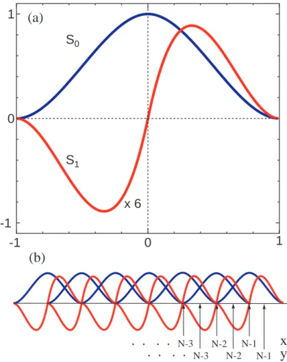
where the spacing is determined by d ≡ xmax/(N − 1), and S0 and S1, shown in Fig. 1(a), are defined by S0(x) = 1 − 3x2+ 2x3, 0 ≤ x ≤ 1 S0(−x), −1 ≤ x < 0 0, otherwise (8) S1(x) = x − 2x2+ x3, 0 ≤ x ≤ 1 −S1(−x), −1 ≤ x < 0 0, otherwise (9)
The spline function S0 satisfies a set of conditions that S0(0) = 1, S00(0) = 0, and S0(±1) =
S0
0(±1) = 0, while S1 satisfies S1(0) = 0, S10(0) = 1, and S1(±1) = S10(±1) = 0. The superscript (i) for Sk(i) in Eq. (7) means that the origin of Sk is shifted to xi, where xi is
given by id. The accuracy in description of R can be systematically controlled by increasing
N as shown later. Employing Eq. (7) for Eq. (2) readily gives the following generalized
eigenvalue problem:
Hc = εSc, (10)
where H and S are the hamiltonian and overlap matrices, respectively, and these matrices becomes septuple diagonal in LDA, since basis functions S(i) interact with basis functions
S(i±1) in the nearest neighbor sites i ± 1. All the matrix elements, except for that of the
exchange-correlation potential such as LDA,[25, 26] can be analytically evaluated. For ex-ample, all the non-zero matrix elements for the operator ˆT0 are found to be
off-site elements hS0(i)| ˆT0|S0(i+1)i = −3d2 280 (5 + 24i + 42i 2+ 28i3), (11) hS0(i)| ˆT0|S1(i+1)i = d2 560(−5 − 12i + 14i 3), (12) hS1(i)| ˆT0|S0(i+1)i = −d2 560(7 + 30i + 42i 2+ 14i3), (13) hS1(i)| ˆT0|S1(i+1)i = −d2 3360(11 + 36i + 42i 2+ 28i3), (14)
-1 0 -1 0 1 x 6 S0 S1 1 N-1 N-1 N-2 N-3 N-2 N-3
. . . .
. . . .
y
ix
i(a)
(b)
Figure 1: (Color online) (a) Cubic Hermite spline functions S0 and S1 defined by Eqs. (8) and (9). (b) Two sorts of regular meshes {xi} and {yi} in x-coordinate, which are used for
fitting of the hartree and exchange-correlation potentials.
on-site elements for i 6= 0
hS0(i)| ˆT0|S0(i)i = 3d2
35(6i + 7i
3), (15)
hS0(i)| ˆT0|S1(i)i = hS1(i)| ˆT0|S0(i)i =
d2 40(1 + 6i 2), (16) hS1(i)| ˆT0|S1(i)i = d2 105(3i + 7i 3), (17)
on-site elements for i = 0
hS0(0)| ˆT0|S0(0)i = 15d2 208 , (18) hS0(0)| ˆT0|S1(0)i = hS1(0)| ˆT0|S0(0)i = d2 80, (19) hS1(0)| ˆT0|S1(0)i = 11d2 3360. (20)
It turns out that the matrix elements depend on the site i as a result that the extent of region spanned by the basis function in r-coordinate varies depending on the site i. Also it is noted that four on-site matrix elements at i = 0 have to be calculated by taking account of a fact that the basis functions S(0) span only the region ranging from 0 to d in x-coordinate, resulting in Eqs. (18)-(20). As well as ˆT0, the matrix elements for ˆT1, −Z/x2, and VH(x) and the overlap matrix elements can be analytically evaluated, and all the analytic formulas and Mathematica codes for generating them are provided in Secs. S-1-12 of the supplemental material. Although the matrix elements for VHcan be analytically evaluated as shown in the section of HF method, for the LDA calculation we present an alternative numerical method which is much faster than the analytic counterpart, while keeping numerical accuracy. Thus, one may see that in LDA the remaining matrix elements which are numerically evaluated are only those for the hartree and exchange-correlation potentials in the FE method.
Here we show that even the matrix elements for the hartree and exchange-correlation potentials can be very accurately evaluated by utilizing the same cubic spline functions in the FE method. Let us introduce two sorts of regular meshes with spacing d in x-coordinate, that is, one is xi as defined before and the other yi ≡ d(i + 12), as shown in Fig. 1(b).
We evaluate the charge density n on the two regular meshes, where, by recalling that the basis functions are strictly localized in real space, one can compute the charge density n by considering only contributions of the neighboring sites at each mesh point, and fit the charge density on the meshes to the following function:
n(x) = N −1X i=0 µ aiS0(i)( x − xi d ) + biS (i) 1 ( x − xi d ) ¶ , (21)
where ai and bi are uniquely determined by a set of recurrence formulas:
ai = n(xi), (22) bi = 8n(yi) − 4ai, i = N − 1
8n(yi) − 4ai− 4ai+1+ bi+1, i 6= N − 1,
(23) The recurrence formulas are derived by noting that only S0(i) is non-zero at xi as shown in
Fig. 1(b) and that bi is only the unknown parameter if we start to fit {Vxc(yi)} to the function
Eq. (21) from yN −1, which results in that Eq. (23) has to be recursively solved starting from
i = N − 1. Once n is expanded in terms of the Hermite spline functions, by considering the
spherical charge density distribution, we can analytically evaluate the hartree potential as
VH(xi) = 8π x2 i Z xi 0 n(x 0)x05dx0+ 8πZ ∞ xi n(x0)x03dx0, (24)
where the integrals are analytically evaluated due to the integrands by simple polynomial functions. As well, {VH(yi)} on the other mesh yi are calculated in the same way as for
{VH(xi)}. The explicit formulas of the integrals can be found in Secs. S-13 and 14 of the
supplemental material. Using the similar way to the expansion of charge density, the set of
{VH(xi)} and {VH(yi)} can be fitted to
VH(x) = N −1X i=0 µ AiS0(i)( x − xi d ) + BiS (i) 1 ( x − xi d ) ¶ , (25) where the coefficients Ai and Bi are uniquely determined by the similar recurrence formulas
to Eqs. (22) and (23). Once {VH(xi)} and {VH(yi)} are fitted to Eq. (25), the calculation of
matrix elements for VH(x) is straightforward as follows:
hSk(i)|VH|Sk(j)0 i = N −1X p=0 ³ AihSk(i)|S (p) 0 |Sk(j)0 i + BihSk(i)|S1(p)|Sk(j)0 i ´ . (26)
The integrals involved survive only if p = i − 1, i, or i + 1 for i = j, and p = i or j for |i − j| = 1, and there are 24 and 16 non-zero elements for the former and the latter, respectively, which can be easily evaluated in analytic formulas. The other combinations give always zero elements due to the strictly localized spline functions. All the analytic formulas and Mathematica codes for generating them are provided in Secs. S-15-21 of the supplemental material. The matrix elements for the exchange-correlation potential can be calculated by just replacing VH with Vxc in Eqs. (25) and (26) after {Vxc(xi)} and {Vxc(yi)} are calculated
by LDA. Thus, from the above derivation we see that all the matrix elements required in the FE method within LDA are evaluated without introducing numerical integration which can be a serious source of numerical error. It is also pointed out that the extension of the method to generalized gradient approximation (GGA)[27] has no difficulty. We only have to perform the evaluation of Vxc by GGA instead of LDA.
Since the resultant hamiltonian and overlap matrices are septuple diagonal, the eigenval-ues and eigenstates can be efficiently calculated by a combination of a shift-and-inverse Lanc-zos method and a shift-invert method,[29] which are used to estimate approximate eigenstates and to refine the approximate eigenstates, respectively. To calculate approximate eigenstates by the shift-and-inverse Lanczos method, the generalized eigenvalue problem Eq. (10) is now transformed to
where the transformed hamiltonian H0, eigenvalues λ, and eigenvectors c0 are given by H0 = (H − ε 0S)−1, (28) λ = 1 ε − ε0 , (29) c0 = Sc. (30)
The shift ε0 for the eigenvalues is taken to be an approximate lowest eigenvalue for each angular momentum l, which can be found from the results at the previous self-consistent field (SCF) step. Then, the Lanczos iteration for Eq. (27) is performed by the following recurrence formulas: αn = hun|H0|uni, (31) |rni = SH0|uni − βn|un−1i − αn|uni, (32) βn+1 = q hrn|S−1|rni, (33) |un+1i = |rni/βn+1, (34)
where the initial vector |u0i is generated by random numbers, but normalized with respect to S−1. The multiplication between a matrix and a vector, (H − ε
0S)−1|uni and S−1|uni,
can be calculated by making use of the LU and Cholesky factorizations, respectively, in O(N) operations. The recursion level of 100-200 is used to obtain sufficient convergence. By diagonalizing the tridiagonal matrix of which diagonal elements are αn and the off-diagonal
elements are βn, and back-transforming {λ} and {c0} by Eqs. (29)-(30), one can obtain a
set of approximate eigenvalues {ε} and eigenvectors {c} starting from the lowest state. The approximate eigenvalues {ε} and eigenvectors {c} obtained by the shift-and-inverse Lanczos method can be further refined by the following shift-invert method:
|dn+1i = (H − εnS)−1S|cni, (35) εn+1 = εn+ 1 hcn|S|dn+1i , (36) |cn+1i = |dn+1i hdn+1|S|dn+1i , (37)
where one of the approximate vectors, corresponding to an occupied state, is chosen as the initial vector |c0i. The iteration is repeated until a condition |εn+1− εn| < 10−16is satisfied.
Only less than 10 iterations are enough to achieve the condition for each eigenstate. It is also noted that the shift-and-inverse Lanczos method can be skipped as the SCF iteration converges, since the eigenvectors found at the previous SCF step are good approximation for the shift-invert method at the next SCF step, which allows us to accelerate the calculation.
2.2
HF method
The difference between the LDA and HF methods lies in treatment of the exchange potential. In the HF method, the following potential is used instead of Eq. (6)
ˆ
V = −Z
x2 + VH(x) + ˆVX, (38)
where ˆVX is the nonlocal exchange operator which acts as
ˆ VXψα(r) = occ. X β Z d3r0ψ∗ β(r0) 1 |r − r0|ψα(r 0)ψ β(r). (39)
One can analytically evaluate matrix elements for the nonlocal exchange potential thanks to the simple polynomial of the Hermite spline functions. In addition, the matrix elements for the hartree potential are also analytically evaluated to keep consistency in evaluating the matrix elements for the hartree and exchange potentials in the HF method, while the matrix elements are evaluated in an alternative way in the LDA calculation. To evaluate the exchange potential with the one particle wave functions Eq. (1), the Coulomb operator is expanded in terms of the spherical harmonics
1 |r − r0| = ∞ X λ=0 λ X µ=−λ Ã rλ < rλ+1 > ! Y∗ λµ(ˆr)Yλµ(ˆr0), (40)
where r> and r< are the greater and lesser of r and r0, respectively. By using the expansion
of the radial function Eq. (7) along with Eq. 40, the exchange energy is computed as follows:
EX = 12 P αhψα| ˆVX|ψαi =Plmax l=0 PN −1 i1,i2=0 P1 k1,k2=0ρ l i1,k1,i2,k2hS (i1) k1 , l| ˆVX|S (i2) k2 , li (41)
where ρ is the spherically averaged density matrix for each l channel
ρl i,k,i0,k0 = (2l + 1) occ. X n0l0 δll0c(n 0l0) ik c (n0l0) i0k0 , (42) and hS(i1) k1 , l| ˆVX|S (i2)
k2 , li is l-dependent matrix elements of the exchange potential in a
repre-sentation with the Hermite spline basis functions. Similarly, the Hartree energy is computed as EH = Plmax l=0 PN −1 i1,i2=0 P1 k1,k2=0ρ l i1,k1,i2,k2hS (i1) k1 | ˆVH|S (i2) k2 i, (43)
with l-independent matrix elements hS(i1)
k1 | ˆVH|S
(i2)
k2 i. After performing the integration in the
angular coordinates, the matrix elements of ˆVH and ˆVX, which are parts of the hamiltonian
matrix elements, are obtained as
hS(i1) k1 |VH|S (i2) k2 i = lXmax l0=0 1 X k3,k4=0 N −1X i3,i4=0 ρl0 i3,k3,i4,k4h13|24iλ=0, (44)
and hS(i1) k1 , l| ˆVX|S (i2) k2 , li = − 1 2 lXmax l0=0 1 X k3,k4=0 N −1X i3,i4=0 ρli03,k3,i4,k4 × l+l0 X λ=|l−l0| Cl0 l,λh13|42iλ, (45)
where the coefficient Cl0
l,λ is Cl0 l,λ ≡ (2l+1)(2l4π0+1)(2λ+1) Pl m=−l Pl0 m0=−l0 Pλ µ=−λ (R dΩrYl∗0m0(ˆr)Ylm(ˆr)Yλµ(ˆr))2, (46)
and the quantity denoted by a closed bracket is the two-electron integrals
htu|vwiλ ≡ Z ∞ 0 dr Z ∞ 0 S (it) kt (r)S (iu) ku (r 0) Ã rλ+2 < rλ−1 > ! ×S(iv) kv (r)S (iw) kw (r 0) = 4 Z ∞ 0 dx Z ∞ 0 dx 0x3−2λ > x5+2λ< ×S(it) kt (x)S (iu) ku (x 0)S(iv) kv (x)S (iw) kw (x 0). (47)
The factor of a half in Eq. 45 appears because degenerate spin configurations are assumed here. Note also in Eq. 45 that the summation over λ is truncated due to the fact that the coefficient Cl0
lλ is always zero when λ > l + l0 or λ < |l − l0|. The integral 47 is invariant under
the following rotations of indices
h12|34iλ = h32|14iλ = h14|32iλ = h34|12iλ
= h21|43iλ = h41|23iλ = h23|41iλ = h43|21iλ. (48)
Due to this invariance, the ordering among the mesh indices
i1 ≤ i3, i1 ≤ i2 ≤ i4, (49) can be assumed without losing generality. Furthermore, by considering that the integral has a non-zero value only when i1 and i3 specify the same mesh point or the neighboring points with each other, and so are i2 and i4, it is also possible to assume
i3 ≤ i4. (50)
To summarize above, one can safely assume that
and
i2 = i4 or i4− 1, i3 = i1 or i1+ 1. (52) This is validated because the integral is always zero whenever Eqs. 51 and 52 cannot be satisfied simultaneously under any rotation in Eq. 48. Then, within this assumption, the integration ranges for x and x0 in Eq. 47 are
x ∈ [x0, x1], x0 = d(i3− 1), x1 = d(i1+ 1), (53)
x0 ∈ [x0
0, x01], x00 = d(i4− 1), x01 = d(i2+ 1). (54) These ranges may and may not overlap with each other. The simpler case is when x1 ≤ x00 or, equivalently, i4 ≥ i1+ 2 and thus they have no overlap. In this case, the integral is given as h12|34iλ = 4d10D5+2λi1,k1,i3,k3D 3−2λ i2,k2,i4,k4, (55) where Dl i,k,i0,k0 ≡ Z i+1 i0−1 dt t lS k(t − i)Sk0(t0− i0). (56)
Note that the integration range is bounded to be non-negative. Therefore, the actual lower limit of the above integral is sup(i0 − 1, 0), although we denote it as i0 − 1 for simplicity.
Readers must keep in mind that the similar notations are also used in the following equations. For the other case where x1 > x00 or, equivalently, i4 = i1 or i1+ 1, the ranges have overlap with each other for
x ∈ [x0
0, x1]. (57)
Then, the integral is given as
h12|34iλ = 4d10 ³ L5+2λ,i4 i1,k1,i3,k3D 3−2λ i2,k2,i4,k4 + Q λ {it},{kt} + Di5+2λ1,k1,i3,k3R3−2λ,i1 i2,k2,i4,k4 ´ , (58) where Qλ{it}{kt} ≡Ri1+1 i4−1 dt Ri1+1 i4−1 dt 0 t5+2λ < t3−2λ> Sk1(t − i1) ×Sk2(t0− i2)Sk3(t − i3)Sk4(t0− i4), (59) Lλ,i4 i1,k1,i3,k3 ≡ Ri4−1 i3−1 dt t λS k1(t − i1)Sk3(t − i3), (60) Rλ,i1 i2,k2,i4,k4 ≡ Ri4+1 i1+1 dt t λS k2(t − i2)Sk4(t − i4). (61)
All the integrals D, Q, L and R in Eqs. 56, 59, 60 and 61, respectively, can be analytically solved. For example, the integral D with l = 5 are:
When i0 = i = 0, D5 0,0,0,0 = 19807 , (62) D5 0,0,0,1 = D50,1,0,0= 1386013 , (63) D50,1,0,1 = 1 3960. (64) When i0 = i > 0, D5 i,0,i,0 = 26i 5 35 +38i 3 63 +775i, (65) Di,0,i,15 = D5 i,1,i,0 = i 4 6 + 4i 2 63 +693013 , (66) D5 i,1,i,1 = 66i 5+110i3+15i 3465 . (67) When i0 = i + 1, D5 i,0,i+1,0 = 9i 5 70 + 9i4 28 + 23i3 63 + 19i2 84 + 23i 308 + 41 3960, (68) D5 i,0,i+1,1 = −13i 5 420 − i 4 14− 19i 3 252 − 11i 2 252 −184825i −39607 , (69) D5i,1,i+1,0 = 13i5 420 + i 4 12+ 25i 3 252 +4i 2 63 +79217i + 3301 , (70) D5 i,1,i+1,1 = −i 5 140 − i4 56− 5i3 252 − i2 84 − i 264 − 1 1980. (71)
It turns out that the combinations of the mesh indices which gives non-zero values of Q are classified into the following cases
Case 1: i1 = i2 = i3 = i4 = 0 Case 2: i1 = i2 = i3 = i4 > 0 Case 3: i1 = i2 = i, and i3 = i4 = i + 1 Case 4: i1 = i2 = i3 = i, and i4 = i + 1 Case 5: i1 = i, and i2 = i3 = i4 = i + 1 Case 6: i1 = i3 = i, and i2 = i4 = i + 1
and otherwise Q is zero. All the analytic formulas for D, Q, L, and R and Mathematica codes for generating them are provided in Sec. S-22 of the supplemental material.
Since the exchange term is nonlocal, the hamiltonian is not septuple diagonal. Therefore, one cannot apply the same techniques as the LDA calculations to solve the generalized eigen-value problem. However, by noting that the septuple diagonal elements in the hamiltonian are still dominant, the refinement procesure can be generalized even for the dense hamilto-nian matrix in the HF method. To derive the generalized method, we first divide H and εS into H = HSD+ (H − HSD) and εS = (ε − ε0)S + ε0S, where HSD is the septuple diagonal
hamiltonian and ε0 is a reference energy. By putting these expressions into Eq. (10), one can derive the following equation:
c = (ε − ε0)(HSD− ε0S)−1Sc
−(HSD− ε0S)−1(H − HSD)c. (72)
Based on the equation, the shift-invert method of Eqs. (35)-(37) can be generalized as follows:
|dn+1i = (HSD− εnS)−1S|cni, (73) |en+1i = (HSD− εnS)−1(H − HSD)|cni, (74) εn+1 = εn+ 1 + hcn|S|en+1i hcn|S|dn+1i , (75) |fn+1i = (εn+1− εn)|dn+1i − |en+1i, (76) |cn+1i = |fn+1i hfn+1|S|fn+1i , (77)
where one of the approximate vectors for an occupied state is chosen as the initial vector |c0i. As well as the shift-invert method by Eqs. (35)-(37), one can achieve sufficient convergence by only less than 10 iterations by Eqs. (73)-(77). The matrix multiplication with (HSD− εnS)−1
is performed by making use of the LU factorization in O(N) operations as in the LDA calculation. We employ the conventional scheme for the diagonalization in the initial stage of the SCF calculation, and switch it to the above shift-invert method after several SCF iterations, which accelerates the calculation, since a few eigenstates only have to be evaluated in the scheme.
3
NUMERICAL ACCURACY
The numerical accuracy of the solution for the Schr¨odinger equation can be evaluated by the virial theorem. If the solution is exact, the virial theorem rigorously holds. Thus, the numerical deviation in the virial theorem is a measure of examining numerical error of the solution. Considering that the correlation energy in LDA includes a part of kinetic energy, the virial theorem for LDA is defined by
2³Ekin+ Ekin(c)
´
where Ekin and Epot are the conventional kinetic and potential energies in LDA. The contri-bution from the correlation energy to the kinetic energy, Ekin(c), is given by
Ekin(c) =
Z
n(r)tc(n)dr (79) with the definition of an energy density
tc= 3µc− 4εc, (80) where εc is the correlation energy density, and µc ≡ d(nεc)/dn. The expressions, Eqs. (78)-(80), for the virial theorem can be derived as shown in Ref. [30] by using the generalized procedure by Slater.[31] On the other hand, the virial theorem simply holds in the HF method without any correction.
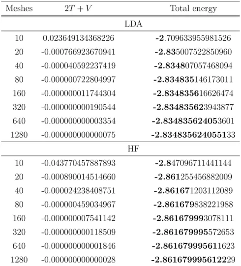
In Table I we show the convergence of the virial theorem and the total energy for the LDA and HF calculations of a helium atom as a function of the number of meshes, where
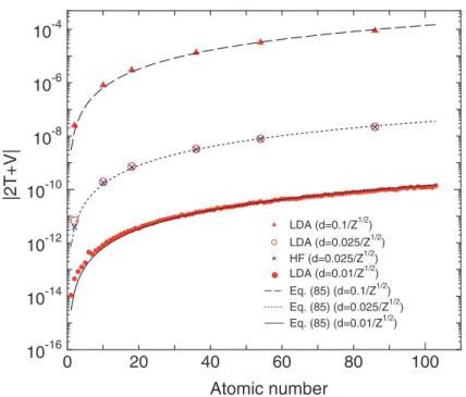
xmax of 10 bohr1/2 is used as the maximum range of x-coordinate for all the cases. The analytic functional form parametrized by Vosko, Wilk, and Nusair[26] is used for the LDA calculations. All the calculations in the study are performed using long double of 80 bit which has 19 significant digits decimally. It is found that the errors in the virial theorem and the total energy for the both cases algebraically decay as the number of meshes increases. Also we see that the order of the errors in the virial theorem and the total energy are almost equivalent to each other, which supports that the evaluation of the virial theorem can be a measure of checking the accuracy of the total energy. Using 1280 mesh points, corresponding to d = 10/1280 bohr1/2, the total energy is calculated with accuracy of 14 digits for the LDA and HF calculations.[32] It is worth mentioning that the total energy converges from above as the number of meshes increases for both the LDA and HF calculations, which indicates that the method can be regarded as a variational method in practice. We further verify the accuracy of the method by applying the FE method to all the atoms (Z=1-103) in the periodic table within LDA and a series of rare gas atoms within the HF method,[33] where the spherical charge density distribution is assumed for the non-spin polarized ground state electronic configuration in the LDA calculations. Figure 2 shows the absolute value of the virial theorem, |2T + V |, as a function of atomic numbers. By considering that the eigenenergies of hydrogen like atoms scales as Z2, the mesh spacing d are taken to be inversely proportional to √Z so that the bare Coulomb potential −Z/x2 at x
1 can be proportional to Z2. The error in the virial theorem for the LDA calculations with the mesh spacing of 0.01/√Z is 1.1 × 10⁻¹⁴ and 1.3 × 10⁻¹⁰ hartree for hydrogen and lawrencium atoms,
respectively, and the errors of the other cases are in between those of the two atoms, which suggests that using the mesh spacing the total energy for LDA can be computed within
Table 1: The virial theorem and the total energy in hartree calculated by the LDA and HF methods for the ground state of a helium atom. xmax of 10 bohr1/2 is used as the maximum range of x-coordinate. The bold font means that the number is exact.
Meshes 2T + V Total energy
LDA 10 0.023649134368226 -2.709633955981526 20 -0.000766923670941 -2.835007522850960 40 -0.000040592237419 -2.834807057468094 80 -0.000000722804997 -2.834835146173011 160 -0.000000011744304 -2.834835616626474 320 -0.000000000190544 -2.834835623943877 640 -0.000000000003354 -2.834835624053601 1280 -0.000000000000075 -2.834835624055133 HF 10 -0.043770457887893 -2.847096711441144 20 -0.000890014514660 -2.861255456882009 40 -0.000024238408751 -2.861671203112089 80 -0.000000459034967 -2.861679838221988 160 -0.000000007541142 -2.861679993078111 320 -0.000000000118509 -2.861679995572653 640 -0.000000000001846 -2.861679995611623 1280 -0.000000000000028 -2.861679995612229
error of 10−9 hartree for all the atoms in the periodic table. In addition to |2T + V |, we
also check a variant of the virial theorem |V /T + 2| (not shown), and find that |V /T + 2| is about 10−14 for all the atoms, indicating that the relative error is almost constant and
the number of accurate digits of the total energy is almost equivalent to each other, which is 13-14 digits in the case of the mesh spacing of 0.01/√Z. It is also confirmed that all the
calculated results by LDA are consistent with the results by Kotochigova et al.[34] The error in the virial theorem in the HF calculations with the mesh spacing of 0.025/√Z varies in
a similar way to that of the LDA calculations. The same analysis as the LDA case implies that the total energy of the HF calculations can be obtained within error of 10−7 hartree
and that the number of accurate digits of the total energy is 11-12 digits for all the rare gas atoms in the case of the mesh spacing of 0.025/√Z. The LDA calculations with the coarse
0 20 40 60 80 100 10-16 10-14 10-12 10-10 10-8 10-6 10-4 Atomic number |2T+V| LDA (d=0.01/Z1/2) LDA (d=0.025/Z1/2) HF (d=0.025/Z1/2) LDA (d=0.1/Z1/2) Eq. (85) (d=0.01/Z1/2) Eq. (85) (d=0.025/Z1/2) Eq. (85) (d=0.1/Z1/2)
Figure 2: (Color online) The absolute value (hartree) of the virial theorem, |2T + V |, as a function of atomic numbers calculated by the LDA and HF methods, and correspond-ing curves of error estimated by Eq. (85). The non-spin polarized ground state electronic configuration is considered for all the cases, and the spherical charge density distribution is assumed in the LDA calculations. The mesh spacing d is taken to be 0.01/√Z, 0.025/√Z,
0.1/√Z bohr1/2. x
max of 10 bohr1/2 is used as the maximum range of x-coordinate for all the cases.
mesh spacing are also presented for comparison, showing that the error in the HF calculation is comparable to the corresponding LDA calculation if the same grid spacing is used. The comparison leads to another conclusion that the numerical fitting of exchange-correlation and hartree potentials in the LDA calculations is not a source of numerical errors. In both the LDA and HF calculations the error in the total energy mainly comes from expansion of the wave functions by the finite basis functions.
We now derive a formula which gives the absolute error in the total energy calculated by the FE method. In this derivation it is assumed that a large xmax is used so that the truncation of tail of wave functions cannot be a source of numerical error. The calculation in Fig. 2 suggests that xmax of 10 bohr1/2 is large enough to avoid the error for all the elements (Z=1-103) in the periodic table. From the two observations that the error decreases algebraically as the mesh spacing decreases in Table I, and that the number of accurate digits of the total energy is nearly constant when the mesh spacing is taken to be inversely proportional to √Z, the number of accurate digits of the total energy, Nd, may be written
as
Nd = a log10
³√
Zd´+ b, (81)
where a and b are parameters to be fitted, and d is the mesh spacing as discussed before. Even if we have the same number of accurate digits of the total energy for different elements, the absolute error in the total energy depends on the absolute magnitude of the total energy. Therefore, as the next step, let us roughly estimate the total energy of atoms. Suppose that the total energy can be estimated by the sum of eigenvalues of hydrogen like atoms. Then, the total energy of an atom in which electrons fully occupy all the states up to the principal quantum number nmax is obtained by
E ∝ nXmax n=1 n−1X l=0 (2l + 1)(−Z2 n2) = −nmaxZ 2. (82)
In the case, the atomic number Z is calculated by
Z = nXmax n=1 n−1X l=0 2(2l + 1), = 2 3n 3 max+ n2max+ 1 3nmax (83)
which gives nmax ∝ Z1/3 as Z increases. Substituting the asymptotic form nmax ∝ Z1/3 for Eq. (82), we have
E ∝ −Z7/3. (84)
Noting that the number of accurate decimal places is given by Nd − log10|E|, and using Eqs. (81) and (84), one can derive the following expression to estimate the absolute error,
Eerr, in the total energy,
Eerr = 10−(Nd−log10|E|),
= αZ
7/3
10b(√Zd)a, (85)
where a, b, and α are found to be -6, 2, and 0.3 by fitting Eq. (85) to the data shown in Fig. 2. As shown in Fig. 2 the estimated error by Eq. (85) fits well with that in the whole range we study. Strictly speaking, the expression of Eq. (85) estimates the error in the the virial theorem, since the fitting is done using the virial theorem |2T + V |. However, the expression can be used to estimate the error in the total energy due to the near equivalence of the error between the virial theorem and the total energy. The expression implies that the error in the total energy approximately scales as Z16/3 or d6 when d or Z are fixed.
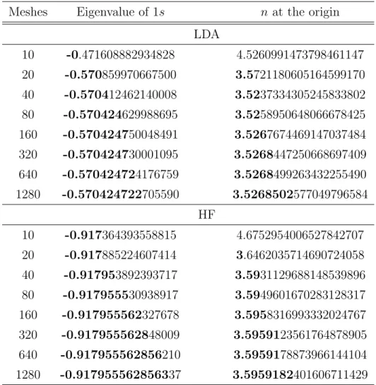
Table 2: The eigenvalue (hartree) of 1s state and charge density at the origin in the ground state of a helium atom. xmax of 10 bohr1/2 is used as the maximum range of x-coordinate. The bold font means that the number is exact.
Meshes Eigenvalue of 1s n at the origin
LDA 10 -0.471608882934828 4.5260991473798461147 20 -0.570859970667500 3.5721180605164599170 40 -0.570412462140008 3.5237334305245833802 80 -0.570424629988695 3.5258950648066678425 160 -0.570424750048491 3.5267674469147037484 320 -0.570424730001095 3.5268447250668697409 640 -0.570424724176759 3.5268499263432255490 1280 -0.570424722705590 3.5268502577049796584 HF 10 -0.917364393558815 4.6752954006527842707 20 -0.917885224607414 3.6462035714690724058 40 -0.917953892393717 3.5931129688148539896 80 -0.917955530938917 3.5949601670283128317 160 -0.917955562327678 3.5958316993332024767 320 -0.917955562848009 3.5959123561764878905 640 -0.917955562856210 3.5959178873966144104 1280 -0.917955562856337 3.5959182401606711429
As well as the convergence property of the total energy, the eigenvalue of 1s state and the charge density at the origin in the ground state of a helium atom are shown as a function of the number of meshes in Table II. Although these quantities slowly converge compared to the total energy shown in Table I, it can be seen that the systematic convergence produces highly accurate results for both the LDA and HF calculations.
4
CONCLUSIONS
We have developed an accurate FE method for atomic calculations based on DFT within LDA and the Hartree-Fock method. Cubic Hermite spline functions on a uniform mesh for
integrations being a source of numerical error can be avoided due to the simplicity of the cubic Hermite spline functions, and all the associated integrals are analytically evaluated in conjunction with fitting of the hartree and exchange-correlation potentials to the same cubic Hermite spline functions. By taking account of the localized nature of the basis functions in real space, the generalized eigenvalue problem is efficiently solved using a generalized shift-invert iterative method for not only the LDA but also HF calculations. The numerical calculations show that the convergence is systematically controlled by the mesh spacing and in practice numerically exact solutions can be obtained within machine precision for all the elements (Z=1-103) in the periodic table. The convergence of the total energy from above implies that the FE method can be regarded as a variational scheme with respect to the Hermite spline functions for both the LDA and HF methods. Based on the virial theorem and an intuitive analysis the absolute error in the total energy is estimated to be proportional to Z16/3/d6. The absolute error is less than 10−7 hartree for the LDA and HF calculations
when the mesh spacing d is taken to be 0.025/√Z bohr1/2. Since the FE method can provide high quality numerical solutions with a similar degree of accuracy for both DFT and the HF method, this can be utilized as a platform, which is free from the non-intrinsic numerical error in the validation of newly developed methods, for development of new functionals in DFT such as hybrid functionals. Along this line, we have been trying to develop a hybrid exchange hole model based on the FE method, which will be discussed elsewhere.
ACKNOWLEDGMENT
The authors were partly supported by the Fujitsu lab., the Nissan Motor Co., Ltd., Nip-pon Sheet Glass Co., Ltd., and the Next Generation Super Computing Project, Nanoscience Program, MEXT, Japan.
References
[1] J.C. Slater, Quantum Theory of Atomic Structure, Vol. 1, McGraw-Hill, New York, 1960.
[2] J.C. Slater, Quantum Theory of Atomic Structure, Vol. 2, McGraw-Hill, New York, 1960.
[3] D. Feller, K.A. Peterson, and T.D. Crawford, J. Chem. Phys. 124 (2006) 054107. [4] R.M. Martin, Electronic Structure: Basic Theory and Practical Methods, Cambridge
[5] T. Helgaker, P. Jorgensen, and J. Olsen, Molecular Electronic-Structure Theory, Wiley, 2000.
[6] C.E. Dykstra, G. Frenking, K.S. Kim, and G.E. Scuseria, Theory and Applications of
Computational Chemistry: The First 40 Years (A Volume of Technical and Historical Perspectives), Elsevier, Amsterdam (2005).
[7] B.W. Shore, J. Chem. Phys. 58 (1973) 3855.
[8] J.L. G´azquez and H.J. Silverstone, J. Chem. Phys. 67 (1977) 1887. [9] C.F. Fischer and W. Guo, J. Comp. Phys. 90 (1990) 486.
[10] H.T. Jeng and C.S. Hsue, Chin. J. Phys. 35 (1997) 215.
[11] Z. Romanowski, Modelling Simul. Mater. Sci. Eng. 16, 015003 (2008); ibid. 17 (2009) 045001.
[12] D. Engel, M. Klews, and G. Wunner, Comp. Phys. Comm. 180 (2009) 302. [13] S.R. White, J.W. Wilkins, and M.P. Teter, Phys. Rev. B 39 (1989) 5819. [14] E. Tsuchida and M. Tsukada, Phys. Rev. B 54 (1996) 7602.
[15] J.E. Pask and P. Sterne, Modelling Simul. Mater. Sci. Eng. 13 (2005) R71. [16] E.J. Bylaska, M. Holst, and J.H. Weare, J. Chem. Theory Comput. 5 (2009) 937. [17] P. Hohenberg and W. Kohn, Phys. Rev. 136 (1964) B864.
[18] W. Kohn and L. J. Sham, Phys. Rev. 140 (1965) A1133. [19] A.D. Becke, J. Chem. Phys. 98 (1993) 1372.
[20] T. Leininger, H. Stoll, H.-J. Werner, and A. Savin, Chem. Phys. Lett. 275 (1997) 151. [21] H. Iikura, T. Tsuneda, T. Yanai, and K. Hirao, J. Chem. Phys. 115 (2001) 3540. [22] J. Heyd, G.E. Scuseria, and M. Ernzerhof, J. Chem. Phys. 118 (2003) 8207.
[23] T.M. Henderson, A.F. Izmaylov, G. Scalmani, and G.E. Scuseria, J. Chem. Phys. 131 (2009) 044108.
[24] In addition to the change of variables, r = x2, we tried two other cases, r = exp(x) and r = exp(x2) − 1, and found that the latter two cases lead to complication in the formalism.
[25] D.M. Ceperley and B.J. Alder, Phys. Rev. Lett. 45 (1980) 566.
[26] S.H. Vosko, L. Wilk, and M. Nusair, Can. J. Phys. 58, (1980) 1200; S.H. Vosko and L. Wilk, Phys. Rev. B 22, (1980) 3812.
[27] J.P. Perdew, K. Burke, and M. Ernzerhof, Phys. Rev. Lett. 77 (1996) 3865.
[28] In addition to the cubic Hermite spline functions, we investigated the convergence of the quintic Hermite spline functions, and found that the convergence ratio with respect to the total number of basis functions is comparable to the cubic case. Thus, it is concluded that the cubic Hermite spline functions is an optimum choice with respect to the convergence ratio and the simplicity of analytic expressions derived for matrix elements.
[29] Z. Bai, J. Demmel, J. Dongarra, A. Ruhe, and H. van der Vorst, Templates for the
Solution of Algebraic Eigenvalue Problems: A Practical Guide, Society for Industrial
Mathematics (1987).
[30] F.W. Averill and G.S. Painter, Phys. Rev. B 24 (1981) 6795. [31] J.C. Slater, J. Chem. Phys. 57 (1972) 2389.
[32] The total energy we obtain corresponds to that in the nonrelativistic HF limit, which lacks the correlation energy of 0.042044 hartree compared to the exact energy of -2.903724 hartree.
[33] The program code, ADPACK, and the calculated results are available on a web site (http://www.openmx-square.org/).
[34] S. Kotochigova, Z.H. Levine, E.L. Shirley, M.D. Stiles, and C.W. Clark, Phys. Rev. A 55, 191 (1997); a web site of the database