Evaluation of the Effects of Capital Inflows on
the Real Economy and Monetary/ Financial
Sector in Indonesia: Lessons from the
Post-IMF Policy Reform on Capital
Account Management and Controls
Hideaki O
HTA ※Abstract
This paper analyses the effects of the policy changes in capital account liber-alization and controls in Indonesia during the post-IMF program since 2004 and compare the previous period of liberalization regime before/after the Asian Crisis as well as the period under the IMF program in 1994-2003. The analysis based on the VAR (vector autoregressive) and Bayesian VAR models confirmed that capital controls and management of the Indonesian authority have actually worked to stabilize the economy, and to minimize the effects of capital inflows in the markets after the termination of the IMF program during the period 2004-2016Q1. The results indicate that the Indonesian economy has become less dependent on capital flows in the real economy as well as the monetary/ financial sector, which would mitigate the risk of speculative short capital flows since 2004.
Keywords: International Capital Flows, Capital Account Liberalization and Controls, Real Economy, Foreign Exchange and Monetary /Financial Markets
JEL Classification codes: E44, F21, F37, O23, O53
1. Introduction
The issue on capital account management and controls has been recognized as one of the important economic policies among the academics, as well as the parties
※ Professor, College and Graduate School of International Relations, Ritsumeikan University
© The International Studies Association of Ritsumeikan University:
concerned including international organizations especially after the global
finan-cial crisis in 20081. Capital controls and management are important policy tools for
emerging market economies under the current global economies and markets, where massive capital flows have put constant pressure on the economies concerned for the risk of capital account crises.
This paper examines the effectiveness of capital management and controls not only as short-term measures to avoid speculative capital flows, but also medium-to long-term policy tools to achieve stable economic growth and stabilization of the
domestic financial market2. Capital account and foreign exchange controls have
widely been introduced among major emerging economies in Asian countries, in-cluding Indonesia. Indonesia was one of the most seriously affected countries, during the Asian Crisis in 1997/8. With termination of the IMF program in 2003, Indonesia introduced several measures for capital account and foreign exchange controls (e.g. a one-month minimum holding period for certain securities) to stabi-lize the economy since mid-2000s.
One of the major purposes of this paper is to identify the effectiveness of capital controls and regulations in Indonesia, by comparing between the period of liberal-ization under the IMF program and pre- and the post-Asian crisis (1994-2003) with the period after the termination of IMF program (2004-2011) in terms of indepen-dence of monetary policies, including capital / financial controls.
The result of the analysis in this paper shows that several measures of capital controls have worked to stabilize the real economy and the financial market (money stocks, interest rate, and real effective exchange rate) and minimized the negative effects of capital flows on the domestic market since 2004, compared with the period 1994-2003. Among the capital inflow variables, portfolio and other capital inflows, which are usually short-term and speculative in nature, have more positive re-sponse functions of the real economy (GDP growth, production) than that of FDI. This trend is more apparent in the later period (2004-2016Q1) than the previous period over 1994-2003. The impulse response function of ‘other’ capital inflows (mostly external bank loans) have constantly positive for manufacturing in general, including nondurable manufacturing and energy sectors. The impulse response of manufacturing to FDI inflows has positive one in the nondurable and energy based manufacturing especially during the period 2004-2016Q1.
The results indicate that the effectiveness of overall capital controls which have been introduced in Indonesia.
2. Capital Flows and Controls in Indonesia
2. 1 General Overview: the Economy and Capital Flows
Indonesia has achieved stable economic growth especially after the termina-tion of the IMF program in 2003. Several factors, including independent economic policy, as well as monetary and fiscal policy, may have contributed to such a high performance. The global market conditions of mineral resources, including oil and gas prices, have also benefited the Indonesian economy for economic growth since mid-2000s. -10 -8 -6 -4 -2 0 2 4 6 8 10 1990 1995 2000 2005 2010 2015 Surce: IFS database (IMF)
(%, y/y) 1998: -13.1% -10 10 30 50 70 90 110 130 1990 1995 2000 2005 2010 2015
Source: IFS daatabe (IMF) (2010=100)
Fig.1-1: Indonesia: GDP Growth Fig1-2: Indonesia: Manufacturing
Indonesia substantially liberalized the capital/ financial account since 1980s, which is relatively early among the ASEAN countries. The external borrowing from offshore centers, especially Singapore, increased substantially among the non-fi-nancial entities besides banks. Most of the firms had no currency hedging for transactions of foreign exchange, under the inflexible (or nearly fixed) regime of
Rupiah during the period before the Asian Crisis (1997/8)3. In Indonesia Banks and
majority of large firms, which had external debt, had significant loss and suffered from deteriorating balance sheet of those local banks and firms after the Asian Crisis. However, the Indonesian economy has recovered especially since the mid-2000s, and is now joining the club of promising emerging economies after BRICs. It should be noted that it was only after the termination of the IMF program in 2003,
when Indonesia successfully completed early repayment to the IMF.
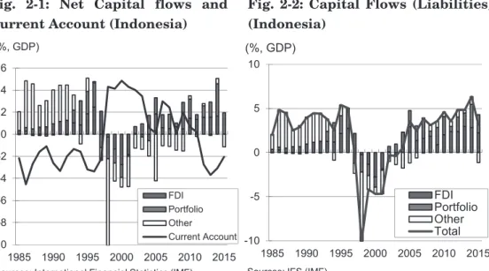
Capital inflows have affected the real economy as well as monetary and finan-cial markets in Indonesia, espefinan-cially in the 1990s. Capital inflows increased signifi-cantly before the Asian Crisis (1997/8), but the net capital outflows accelerated after the crisis. Although the current account improved after the Asian Crisis, it was the result of deterioration of the economy with significant decrease of imports, which put the current account surplus. The balance of payments has broadly improved and the net capital inflows of FDI and portfolio investment continued after 2004 with the stability of the economy.
Indonesia could not introduce extensive capital control measures under the
IMF program4, and it was only after the termination of the IMF program in 2003
that the intensive capital management and controls were undertaken. The domes-tic market has achieved stability since 2004 in terms of the component of the portfolio liabilities, where debt securities have become major component, changed from equity recently (Fig.2-1). The domestic economy and financial market in Indonesia have significantly improved and stabilized since the mid-2000s, even under the expansion of capital flows in the global market in the 2000s. It indicates that the capital market has become relatively stable, since debt securities are generally more stable than stocks or equity securities. Moreover, short-term capital liabilities have decreased significantly since the mid-2000s (Fig.2-2). These recent trends could be explained by the capital management and controls introduced
-10 -8 -6 -4 -2 0 2 4 6 1985 1990 1995 2000 2005 2010 2015 FDI Portfolio Other Current Account (%, GDP)
Sources: International Financial Statistics (IMF)
-10 -5 0 5 10 1985 1990 1995 2000 2005 2010 2015 FDI Portfolio Other Total Sources: IFS (IMF)
(%, GDP)
Fig. 2-1: Net Capital flows and Current Account (Indonesia)
Fig. 2-2: Capital Flows (Liabilities) (Indonesia)
intensively since the mid-2000s, It should be noted that the independence of mon-etary policy with flexibility of policy options after 2004 have made the Indonesian economy more stable and resilient to the external shocks of capital and financial turbulence
2. 2 Capital Account Liberalization and Controls in Indonesia: Historical Overview
As mentioned previously, capital account and foreign exchange controls in Indonesia were liberalized relatively early among the Southeast Asian countries since the latter part of 1980s. The KAOPEN (Chinn-Ito index) which shows capital account openness in each country indicates that Indonesia already started liberal-ization in the 1970s, due to the shortage of foreign exchange from the deterioration
of the current account, as well as increase in the interest rates5 (Fig.4). Major
cap-ital account liberalization measures were introduced mainly in the external trading by individual residents, while the overseas investment by the domestic firms was restricted until the end of 1980s.
Fig. 4: KAOPEN (Asia)
-2 -1 0 1 2 3 1970 1974 1978 1982 1986 1990 1994 1998 2002 2006 2010 2014 China Indonesia Korea Malaysia Thailand Source: 'Chinn-Ito ndex 'H.P. data
Source: 'Chinn-Ito ndex 'H.P. data Source: 'Chinn-Ito ndex 'H.P. data
Intensive liberalization of capital controls was initiated in the early 1990s, which accelerated capital inflows. However, many banks and firms in Indonesia suffered from ‘double mismatch’ of the currency (long-term domestic lending with short-term external borrowing of foreign currency that has foreign exchange risk) before the Asian Crisis (1997/8) in Indonesia. The government authority set the ceiling of the swap amount for non-residents just after the contagion of the Asian Crisis, but it was not effective to prevent the Rupiah currency from falling freely. Although some capital and foreign exchange management and controls were intro-duced, those measures were not introduced during the period of IMF programs (1997-2003), since the IMF in principle took negative approach towards capital
control and management6. During the period of the Crisis, the Government
author-ity introduced banking regulations, and facilitated improvement in the manage-ment of financial institutions under the specialized agency (Indonesian Bank
Restructuring Agency, IBRA)7. However, the Crisis became serious under the IMF
program, which put conditionality of drastic restructuring of the banking sector, including closure of 16 commercial banks.
The policy lesson of the Crisis in Indonesia indicates that a developing country with limited foreign reserves should set limits on its foreign currency debt through
capital and foreign exchange controls and management8.
It was the post-IMF program period since 2004 that the Indonesian govern-ment introduced intensive capital control and managegovern-ment measures. The offshore trading of foreign exchange with Rupiah and the exchange of local currency by the residents, as well as acquisition of foreign assets and the exchange of Rupiah are
now restricted (Table 1)9.
Restrictions of SBI trading for preventing from short-term and speculative in-vestment capital (the policy of One-Month Holding Period, OMHP) were introduced in June 2010, and additional measures including the ceiling of external borrowing and raising the reserve ratio of foreign exchange have been introduced since January 2011. Also, Bank Indonesia introduced regulations to restrict rupiah transactions and foreign currency credit by banks in January 2011.
In principle, all major transactions of foreign exchanges through offshore banks and non-banks are to be reported to the Bank Indonesia. The transactions in the domestic market are to be made by Rupiah currency in principle.
2. 3 Financial / Monetary Markets in Indonesia
The Indonesian Rupiah significantly depreciated during the Asian Crisis, caused by the contagion of the capital outflows from the Asian region triggered by the fall of Thai Baht in July 1997. The real effective exchange rate of Indonesian Rupiah depreciated by 16% until April 1997 from April 1995, and Rupiah depreci-ated significantly as adjustment of the real exchange rate of the currency, which appreciated significantly before the Crisis. However, the level of current account deficit of Indonesia was relatively modest with 2.5% of GDP in the pre-Asian Crisis
(the 2nd quarter of 1996)10. Thus, the current account deficit was not the direct
cause of the Crisis, but rather the contagion of the Crisis triggered by the fall of Thai Baht in July 1997. The fundamental reason, however, was that Indonesia had liberalized capital account regime that was vulnerable to the capital outflows before the Crisis. Significant outflows of capital from financial organizations as well as
Year
1989 Deregulation of ceiling of offshore trading by banks/financial instituions 1989 Foreign investors allowed up to 49% shares
1989 Restriction of net open position(NPO) for forex trading banks/non-banks 1991 Banks' offshore borrowing up to 20% of capital (←25%);
premium for swap for 3 months raised 5%
1991 Approval required for external borrowings by national banks/public corp. 1991 Restriction of the net open positions(NPO) for forex trading banks/non-banks 1992 Allowed foreign investors to acquire a majority of share in commercial banks 1994 Approval required for commericial banks' external borrowins
1994 Deregulation on the net open positions(NPO) for forex trading banks/non-banks 1994 Deregulation on the external commercial borrowings
1995 Restriction on the external borrowings more than 2 years; The share of capital by non-residents to be less than 30%
1996 Foreign investment in mutual funds allowed in 100% foreign owned capital 1997 Future trading of forex to be restrcted less than US$5 million
1997 Liberalization on investment in domestic shares by foreign investors (except banking sector) 1998 Deregulation of prohibited business sectors in FDI
1999 Govt approval not required for M&A
2001 Deregulation on lending of foreign currencies to non-residents by domestic banks 2001 Trading by the domestic banks prohibited;(i)Rupiah denominated overdraft;
(ii)Lending to non-residents; (iii)Transactions of Rupiah-denominated bonds issued by non-residents;(iv) Rupiah trading among non-residents;
(v) Investment in stocks issued by non-residents in Rupiah currency 2004 Stirct regulation on the Reserves in Rupiah in bank accounts 2004 Reporting required for offshore borrowings by financial institutions 2005 Short-term borrowings to be less than 30% of total assets;
Central Bank(Bank Indonesia)'s approval required for lon-term external borrowings 2005 Reserve requirement in Bank Indonesia account raised
2005 Restrction of lending in foreign currencies to non-residents by domesitc banks 2006 Transfers of Rupiah currency to non-residents prohibited
2008 Requirement of report to the Authority on external borrowings from non-residents 2008 Ceiling of conversion of Rupiah to foreign exchange for non-residents over $100,000 monthly
(requirement of special approval for over $100,000)
2008 Conversiton of Rupiah to foreign currency limited for current account transactions in principle 2010 Requirement of holding SBI(Central Bank securities) more than 1 month.
2011 Banks' offshore short-term borrowing up to 30% of capital
Reserve requirement of 5 percent of total foreign-exchange holdings for Banks
All transactions of Banks are to be used by Rupiah; imposed restrictions of foreign currency credit and rupiah transfers to ofshore accounts
2012 Minimum capital raised to Rp10bn for investment (all sectors), and minimum paid in capital with Rp 3bn.
2014 External Borrowings are to be withrwan at thedomesticbanks to be reported at BI. Compulsory minimum hedge ceiling for non-bank firms introduced
2015 Compulsory report on offshore tradings of non-bank firms and financial firms All the transactions(cash/non-cash) in Indonesia should be made in Rupiah currency Note: The shaded area shows foreign exchange and capital controls/regulations
Sources: Author based on the resources of JETRO, Aramaki&Karikomi (2007), Magud&Reinhart(2006), etc.
business firms have resulted in increased external debt burden of banks and do-mestic firms, and the financial crisis accelerated deterioration of the economy.
The exchange rate regime in Indonesia shifted from practically dollar-pegged to more flexible regime after the Asian crisis. As a result, the real effective exchange rate has not appreciated significantly during the past decade, which could be one of the important factors that Indonesia has been able to avoid the risk of currency crisis in the past decade.
Fig.5: Nominal/Real Effective Exchange Rate (Indonesia)
0 20 40 60 80 100 120 0 2,000 4,000 6,000 8,000 10,000 12,000 14,000 16,000 1994 1996 1998 2000 2002 2004 2006 2008 2010 2012 2014 2016 Nominal(LHA) REER(RHA) (Rupiah/$)
Source: IFS (IMF) , BIS (effective exchange rate indices)
Moreover, the foreign exchange and capital controls, the foreign exchange rate has made the Indonesian economy more resilient to the global market conditions, which have been volatile, especially pre- and post-global financial crisis of 2008.
The financial and capital markets have also stabilized, and the money market
0 20 40 60 80 100 120 140 160 180 0 10 20 30 40 50 60 70 80 1995 1998 2001 2004 2007 2010 2013 2016 Interest rate(RHA) M2 (LHA)
Share price (LHA)
(y/y, %) (2010=100)
Source: IFS (IMF)
rate fell to the level of around 4% and stabilized during the first quarter of 2012. The share price also sharply recovered especially in the latter part of 2000s, with stabilization of the economy.It rose again after the Lehman Shock since 2011, though some external factors have affected the level of stock price.
3. Effects of Capital Inflows
3. 1 Past Studies
On the effectiveness of capital controls and management, Goh (2005) indicates that the controls not only reduce the total flows (hence increase monetary autono-my), but to some extent affected the private long-term flows, citing the experience of Malaysia in 1998. The IMF has officially endorsed capital management and controls, as described in the staff notes (see Ostry et al. 2010. 2011), which admitted the effectiveness of capital inflow controls officially for the first time as official documents by the IMF. However, as Habermeier et al. (2011) put it, the IMF has not completely authorize capital controls on outflows of capital and put more em-phasis on macro-prudential measures and market based policy measures on capital management.
In the case of Indonesia, after the termination of the IMF program, the author-ity has strengthened the capital management and financial controls, including prudential measures. The experience of Indonesia may be evaluated from the aca-demic point of view. As shown in this paper, the capital inflows have become limited effects on the Indonesian Economy and the market, and it could be result of the Indonesian authority’s efforts to control the instability of the capital flows especial-ly portfolio investment flows, which is shown in the paper by Bank Indonesia (Hendarsah, 2010).
There are several studies on the effect of capital inflows on economic growth in emerging and developing economies. Among the capital inflows, FDI is generally considered as one of the most important capital resources that could contribute to economic growth in several past studies. Indeed, FDI may raise economic growth in the recipient countries. However, the contribution of FDI to economic growth and expanding productive activities would depend on the circumstances in the recipient countries. Thus, several studies on the effect of FDI on the economy show inconclu-sive results.
Carkovic and Levine (2002), for example, argue that there is not a robust, causal link running from FDI to economic growth. Some empirical study (Alfaro, et
al., 2009, 2010) suggests that FDI could play an important role in contributing to economic growth where financial markets are developed enough; the host country benefits from backward linkages between the foreign and domestic firms. In this regard, Cipollina et al. (2011) suggest that FDI has positive and statistically signif-icant growth effect in recipient countries during 1992-2004, and the effect is stronger in capital intensive and in technologically advanced sectors. These studies indicate FDI could contribute economic growth under certain conditions (matured financial markets, capital and technology intensive sectors, etc.).
Ghosh and Qureshi (2016) also show that while capital inflows generally lead to macroeconomic imbalances and financial vulnerabilities, as well as to a greater likelihood of banking and currency crisis, other investment and portfolio flows (es-pecially portfolio debt flows) are the most risky, while FDI seems to be the safest type of capital inflow, based on a sample of 53 emerging economies over 1980–2013.
In the case of Indonesia, several studies indicate that FDI has limited impact on the economy in terms of economic growth. Dhanani and Hasnain (2002) found that contribution of FDI to economic growth in Indonesia is rather modest in total capital formation and development in industries, and that FDI put negative impact on the balance of payments due to the large propensity to import production inputs from the study in the late 1990s. The study by Effendi and Soemantri (2003) reveals that the effect of FDI on regional economic growth in Indonesia is relatively weak in accelerating the economic growth. These studies suggest that Indonesia may not fully utilize potential benefit of FDI for economic growth.
In terms of capital controls, Blundell-Wignall and Roulet (2014) suggested based on the panel regressions contrast with the idea that controls are most bene-ficial in a crisis, while there was no support for overall controls over the full sample.
This paper confirms the fact that capital inflows, including FDI, had very limited impact upon the real economy in Indonesia, and shows that capital man-agement and controls have contributed to the stability of the economy with rela-tively high growth since 2004 until today. The next section will examine the effects of capital inflows on the real economy and financial, as well as foreign exchange markets, dividing the period between the pre- and post-IMF Program.
3. 2 The Effects of Capital Inflows on the Real Economy and Foreign Exchange, Monetary/Financial Markets: Panel regression
capital controls and regulations introduced after the termination of the IMF pro-grams, to compare the period of liberalization under the IMF program during and after the Asian crisis (1994-2003) with the post-IMF program period during 2004-2016(Q1). Thus, the covered period is divided into the period 1994-2003, and the period 2004-2016(Q1). The latter period covers the period when the government authority became independent from the IMF’s conditionality in economic policy, in terms of monetary and exchange controls/management to stabilize the market and the real economy. The results of regression analyses indicate that the total capital inflows (net) had significant correlation with GDP growth during1994-2003, and the FDI had positive correlation with GDP growth, while portfolio investment had negative with GDP growth.
The regression equations during the period also indicate that the Asian Crisis (Crisis dummy 1) had significantly negative impact upon the GDP growth.
Table 2: Indonesia: Capital Flows and GDP growth [1994-2016] 【Dependent Variable: GDP growth】
6 1 0 2 -4 0 0 2 3 0 0 2 -4 9 9 1 (Q1) 【Explanatory Variables】 (1) (2) (3) (4) (5) (6) (7) (8) (9) (10) (10) 2 6 0 0 . 0 0 0 2 0 . 0 )t e N ( l a t o T ) 5 4 0 . 0 ( ) 3 9 0 . 0 ( ) 0 4 1 . 0 ( ) 4 1 2 . 0 ( 9 8 6 4 . 0 I D F * 0.0867 (% of GDP) (0.263) (0.119) ) 9 2 7 . 0 ( ) 5 8 7 . 1 ( 4 0 1 3 . 0 -o il o ft r o P ** -0.0467 -0.0516 -0.0587 (% of GDP) (0.125) (0.067) (0.062) (0.061) ) 3 6 9 . 0 -( ) 6 2 8 . 0 -( ) 6 9 6 . 0 -( ) 9 7 4 . 2 -( Others 0.2835* 0.0430 (% of GDP) (0.162) (0.053) ) 2 1 8 . 0 ( ) 5 4 7 . 1 ( 2 3 3 1 . 0 R E E R *** 0.047*** (0.031) (0.016) (4.263) (2.865) 4 3 9 . 4 1 -) g o l( 2 M ** -16.385 *** -0.441 (3.002) (2.776) (0.522) ) 5 4 8 . 0 -( ) 2 0 9 . 5 -( ) 5 7 9 . 4 -( 5 7 9 0 . 0 1 6 8 0 . 0 7 1 7 1 . 0 -e t a R t s e r e t n I -0.004
(money market rate) (0.105) (0.094) (0.091) (0.066) (-1.638) (0.921) (1.071) (-0.057) Mfg.Production 0.1783*** 0.1716*** 0.0589 0.0377 0.0621 (0.048) (0.046) (0.043) (0.033) (0.038) (3.695) (3.710) (1.375) (1.154) (1.640) Non-durable Mfg 0.0423 0.0148 0.0326 -0.0310 -0.045 0.0013 0.0017 0.0016 0.0015 (0.043) (0.041) (0.042) (0.035) (0.037) (0.001) (0.001) (0.001) (0.001) (0.980) (0.361) (0.784) (-0.878) (-1.221) (0.890) (1.153) (1.230) (1.093) 9 5 4 5 . 0 s e c ir P li O *** 0.6968*** 0.0124*** (0.158) (0.150) (0.004) (3.461) (4.658) (3.168) Crisis dummy -8.732*** -9.909*** -9.038*** -8.183*** -5.777 *** (1997/8) (2.029) (1.625) (1.826) (1.908) (1.884) -4.3029 -6.0991 -4.9496 -4.2888 -3.066 Crisis dummy -0.4327 -0.6291 -0.5444 -0.5243 (2008/9) (0.427) (0.448) (0.386) (0.402) ) 4 0 3 . 1 -( ) 0 1 4 . 1 -( ) 5 0 4 . 1 -( ) 4 1 0 . 1 -( Constant 4.175*** -5.946* 4.097*** 77.511*** 82.792*** 5.457*** 4.708*** 8.421** 1.420 4.699*** 5.645*** (0.77) (2.83) (0.74) (14.45) (13.28) (0.181) (0.662) (3.300) (1.623) (0.324) (0.125) (5.407) (-2.104) (5.529) (5.362) (6.235) (30.17) (7.115) (2.552) (0.875) (14.48) (45.17) R2 0.7273 0.7467 0.7497 0.8551 0.8289 0.0956 0.1106 0.0565 0.1729 0.2163 0.0810 9 4 0 4 . s b O
Notes 1. Each capital flow variable (Total. FDI, Portfolio, Other investment) are as percentage of GDP 2. Period is between 1994Q1 and 2015Q3.
3. Figures in parentheses are standard deviation (upper) and t-value (lower). Sources: Author's calculation based on database of IFS (IMF) and Bank Indonesia
On the other hand, capital inflows are not statistically correlated with the real economy (GDP growth and manufacturing production) during 2004-2016 (Q1). During the period, real effective exchange rate (REER) and oil price only had sig-nificantly positive correlation with GDP growth. It should be also noted that the Global Financial Crisis (Crisis dummy 2) did not have any significant impact on the GDP growth during the period. It could indicate that capital management and controls introduced during the period might have worked to stabilize the economy and the market in Indonesia.
The regression results show the fact that the real economy (GDP growth) has become more independent from the external capital flows since 2004, as compared with the period 1994-2003.
3. 3 Analysis: Vector Autoregressive Regression (VAR) / Bayesian VAR (BVAR) models
This section is devoted to an analysis of the effects of capital controls on the stabil-ity in the market and the real economy over the period 1994-2016(Q1) through the changes in the response of the shocks of capital inflows (Total, FDI, portfolio, other investment) based on the Vector auto regression (VAR) and Bayesian VAR (BVAR) models.
The impulse response functions based on the VAR model are used to produce the time path of the dependent variables in the VAR, to shocks from all the explan-atory variables. This study estimated the effects of capital inflows on the monetary and financial as well as the real economy in Indonesia based on VAR models com-prising GDP growth rate, financial market indicators (money market rate, money stock [M2]), foreign exchange market (real effective exchange rate), foreign ex-change reserves, manufacturing production index, BVAR method could be used to estimate the response to some shock variables with not sufficient variables, which would be the case in point (as quarterly data). The difference with standard VAR models lies in the fact that the model parameters are treated as random variables, and prior probabilities are assigned to them.
The VAR models in the analysis are classified into the real sector analysis and the financial market, and the former model includes variables of capital flows (Total, FDI, portfolio, other investment; quarterly, percent of GDP), GDP growth [quarterly, y/y], as well as manufacturing. Since the Indonesian economy has been affected significantly by oil/natural gas prices, the variables of manufacturing sec-tors are divided into two variables: total manufacturing and nondurable manufac-turing [including oil/gas sectors]).
The other model includes those variables of capital flows (Total, FDI, portfolio, other investment), the real effective exchange rate [REER], as well the monetary/ financial sectors respectively. Accordingly, the general equations of VAR model are as follows: (1) y1t α1 β1γ1χ1ψ1ω1 y1t-j u1 y2t α2 β2γ2χ2ψ2ω2 y2t-j y3t = α3 + ∑ β3γ3χ3ψ3ω3 y3t-j + u3 u2 y4t α4 β4γ4χ4 ψ4ω4 y4t-j u4
Where the explanatory variables of the regressions (indicated below) are
in-cluded as y1 (t-j indicates the previous period of t).
Variables of capital inflows, namely (i) Total capital inflows (net) of the previ-ous quarter (Total); (ii)Foreign direct investment inflows (net and gross) of the previous quarter (FDI); (iii) Portfolio inflows (net) (Portfolio); (iv) Other investment inflows (Other) are included in the first column of the VAR model.
The variables of the vector in the second and other columns could be any of the following variables: (a) GDP growth rate, (b) manufacturing (total), (c) nondurable manufacturing (including oil/gas and mineral related sectors), (d) real effective exchange rate, (e) money stocks (M2), (f) money market rate, and (g) foreign
re-serves. There are two models involved in the analysis as follows11:
The first model includes those variables of any of the capital inflow variables (Total, FDI, portfolio, other investment) and the real sector of the economy: GDP growth rate; total manufacturing production; nondurable manufacturing produc-tion (incl. oil and other mineral sector)
(i) Capital inflows (Total; FDI; Portfolio; Other investment) (quarterly, per-cent of GDP)
(ii) Manufacturing Production: Changes in total manufacturing production (y/y) [VAR]
Index (2010=100) [Bayesian VAR]
(iii) Nondurable manufacturing (incl. oil/energy sector) production (y/y) (same as (ii))
(iv) Real GDP Growth (y/y) [VAR]; (Index, 2010=100) [BVAR] As an example, the VAR model including total capital flows is shown as follows:
(2)
Totalt α1 β1 γ1 χ1 ψ1 Totalt-j u1
Mfgt = α2 +∑ β2 γ2 χ2 ψ2 Mfgt-j + u2
NDMfg α3 β3 γ3 χ3 ψ3 NDMfgt-j u3
GDPt α4 β4 γ4 χ4 ψ4 GDPt-j u2
The second model includes those variables of any of the capital inflow variables (Total, FDI, portfolio, other investment), and financial/monetary/foreign exchange markets: real effective exchange rate; money stocks (M2); interest rate (money market rate); and Share prices as follows:
(i) Capital inflows (Total; FDI; Portfolio; Other investment) (quarterly, per-cent of GDP)
(ii) Real effective exchange rate (REER) (Index) (iii) Money stocks : M2 (log)
(iv) Money market rate (Intrate) (v) Share prices: Share(Index)
From the above specifications, the VAR model entails 4 times of the equation (3), which has one of the variables other than capital inflow variables. For example, the equation on the Model 2, including Total and the exogenous shock to the other variables, is as follows:
The VAR model including total capital flows sis as follows:
(3) Totalt α1 β1 γ1 χ1 ψ1 ω1 Totalt-j u1 REERt α2 β2 γ2 χ2 ψ2 ω2 REERt-j u2 M2t = α3 +∑ β3 γ3 χ3 ψ3 ω3 M2t-j + u3 Intratet α4 β4 γ4 χ4 ψ4 ω4 Intratet-j u4 Sharet α5 β5 γ5 χ5 ψ5 ω5 Sharet-j u5
3.4.1 ADF test and Stationarity-y
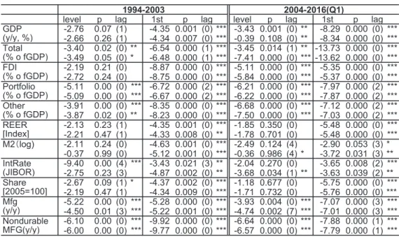
Prior to the analysis based on the VAR model stationarity of the variables in-volved in the regression is tested by ADF (augmented Dickey-Fuller) method for the unit root tests (Table 2).
Capital inflow variables (Total, FDI, portfolio, and other investment), manu-facturing (total and nondurable) production (y/y), as well as GDP growth (for the period 2004-2016Q1) has unit root without first lag. However, the ADF test results show that unit root is not rejected with level for GDP growth (1994-2003) and FDI (1994-2003), so that unit root is rejected for the first lag of each variable, which is
expressed as I (1)12. It should be noted that stationarity of some economic indicators
(GDP growth rate, FDI, REER, share) was not kept without first lag during the period 1994-2003, covering the Asian Crisis period (1997/8). For other variables, the stationarity is confirmed with level, except the variables of REER, LogM2 and Interest rate (Intrate), which are confirmed stationarity with first lag of variables during the whole period (1994-2016Q1).
Table 3: Augumented Dickey-Fuller (ADF)Test (Indoensia)
6 1 0 2 -4 0 0 2 3 0 0 2 -4 9 9 1 (Q1)
level p lag 1st p lag level p lag 1st p lag GDP -2.76 0.07 (1) -4.35 0.001 (0) *** -3.43 0.001 (0) ** -8.29 0.000 (0) *** (y/y, %) -2.66 0.26 (1) -4.34 0.007 (0) *** -0.39 0.108 (0) ** -8.34 0.000 (0) *** Total -3.40 0.02 (0) ** -6.54 0.000 (1) *** -3.45 0.014 (1) ** -13.73 0.000 (0) *** (% o fGDP) -3.49 0.05 (0) * -6.48 0.000 (1) *** -7.41 0.000 (0) *** -13.62 0.000 (0) *** FDI -2.19 0.21 (0) -8.87 0.000 (0) *** -5.11 0.000 (0) *** -5.35 0.000 (0) *** (% o fGDP) -2.72 0.24 (0) -8.75 0.000 (0) *** -5.84 0.000 (0) *** -5.37 0.000 (0) *** Portfolio -5.11 0.00 (0) *** -6.72 0.000 (2) *** -6.21 0.000 (0) *** -7.97 0.000 (2) *** (% o fGDP) -5.09 0.00 (0) *** -6.67 0.000 (2) *** -6.22 0.000 (0) *** -7.87 0.000 (2) *** Other -3.91 0.00 (0) *** -8.35 0.000 (0) *** -6.68 0.000 (0) *** -7.12 0.000 (2) *** (% o fGDP) -3.87 0.02 (0) ** -8.23 0.000 (0) *** -7.50 0.000 (0) *** -7.03 0.000 (2) *** REER -2.13 0.23 (1) -4.35 0.001 (0) *** -1.85 0.350 (0) -5.48 0.000 (0) *** [Index] -2.21 0.47 (1) -4.33 0.008 (0) ** -1.78 0.701 (0) -5.48 0.000 (0) *** M2(log) -2.11 0.24 (0) -4.63 0.001 (0) *** -2.49 0.124 (4) -2.90 0.053 (3) * -0.37 0.99 (0) -5.12 0.001 (0) *** -0.36 0.986 (4) * -3.72 0.031 (3) ** IntRate -9.40 0.00 (4) *** -3.43 0.021 (3) ** -2.04 0.270 (0) -3.65 0.008 (2) *** (JIBOR) -2.75 0.23 (3) -4.87 0.002 (0) ** -3.68 0.034 (1) ** -3.63 0.039 (2) ** Share -2.67 0.09 (1) * -4.37 0.002 (0) *** -1.18 0.677 (0) -5.75 0.000 (0) *** [2005=100] -2.19 0.47 (1) -4.34 0.009 (0) *** -1.71 0.732 (0) -5.76 0.000 (0) *** Mfg -5.22 0.00 (0) *** -5.28 0.000 (0) *** -3.93 0.004 (0) *** -7.07 0.000 (3) *** (y/y) -4.50 0.01 (3) *** -5.22 0.001 (0) *** -4.74 0.002 (7) *** -7.01 0.000 (3) *** Nondurable -6.10 0.00 (0) *** -9.92 0.000 (0) *** -6.64 0.000 (0) *** -7.88 0.000 (1) *** MFG(y/y) -6.00 0.00 (0) *** -9.77 0.000 (0) *** -6.57 0.000 (0) *** -7.79 0.000 (1) *** Notes 1 Upper: Cnstant; Lower: Constant and Trend 2 ***, **, * denotes significance at 1%, 5%, and 10%, respectively. 3. Real Effective Exchange Rate(REER), Foreign Reserves (log). Quarterly Figures.
4.Nondurable: Nondurable Manufacturing indusry ( incl. oil, coal and other energy related sectors) Sources: Author's calculation based on the data of International Financial Statistics (IMF)、BIS(REER)
3. 4. 2 Granger Causality Test
Granger causality tests are essentially those measures to improve in forecast-ing association and correlation between the variables. By usforecast-ing an F-test to jointly test for the significance of the lags on the explanatory variables, this in effect tests
for ‘Granger causality’ between these variables13.
This section focuses on the causality between the variables of capital inflows and foreign exchange rates, monetary and financial markets, as well as the real economy (real GDP growth rate, manufacturing production) based on the quarterly data through VAR model. The analysis is based on the quarterly data of each
variable during the period1994-2016Q1, dividing 1994-2003, and 2004-2016Q1, and the latter period is also divided into the pre-Global Financial Crisis (2004-2008Q2) and the post Global Financial Crisis (2008Q3-2016Q1) to verify the effects of changes in capital inflows in each period. In Indonesia, capital flow management and controls were not significantly introduced, especially under the IMF program continued between 1994 and 2003.
The results of Granger Causality test of each variable, with the average of the
first, 2nd, 3rd and 4th (quarter) lags are summarized in Table4.
Table 4: Granger Causality (Indonesia) [1994-2016(Q1)]
1994-2003 GDP Total FDI Portfolio Other REER M2 Intrate Share Mfg NdMFG 5 2 6 . 2 5 6 1 . 0 5 7 7 . 0 8 2 4 . 0 0 8 3 . 0 P D G * 17.80***2.154 0.587 1.841 1.878 Total 3.093*** 0.842 0.838 6.286***1.120 26.54 *** 2.262 2.093 4.683 ** 0.031 FDI 3.343* 0.425 0.607 2.207 0.886 6.664 ** 0.613 0.666 2.860 * 0.842 Portfolio 1.950 0.197 0.175 10.13 *** 1.326 21.47 *** 1.989 1.375 3.226 * 0.315 Other 5.162***0.149 0.549 0.759 2.328 4.089 ** 1.815 1.643 3.974 ** 0.462 REER 13.58***0.493 0.313 1.023 14.51 *** 12.71 *** 3.283 * 1.973 4.899 ** 0.870 M2 (log) 2.115 0.202 0.796 0.368 8.308 *** 1.038 4.502 ** 0.679 2.257 0.540 Interest rate 15.82***4.652 ** 0.815 9.171***3.030 ** 3.706 ** 2.132 5.742 *** 3.278 ** 2.027 Share 0.799 6.025 *** 1.253 4.792 ** 3.314 2.625 * 1.799 0.505 1.494 0.489 Manufacturing 3.535** 2.086 2.390 0.777 0.510 2.259 0.970 5.041 * 2.539 * 1.648 NdMfg 0.558 0.053 0.546 0.171 0.881 0.079 0.597 0.179 0.334 0.390
2004-2008(Q2) GDP Total FDI Portfolio Other REER M2 Intrate Share Mfg NdMFG 6 3 8 . 4 9 4 0 . 1 6 8 1 . 0 8 0 9 . 1 4 6 7 . 1 5 7 6 . 0 9 2 1 . 1 7 9 2 . 2 8 6 0 . 2 2 7 9 . 0 P D G ** Total 1.225 0.645 1.605 0.502 12.01***1.456 0.679 0.584 0.830 0.332 FDI 1.683 4.568** 1.311 5.391 ** 4.759 ** 2.750 * 0.273 0.102 2.904 * 0.836 Portfolio 0.409 1.523 0.277 0.951 0.878 0.376 0.501 0.534 0.637 1.656 Other 3.696 ** 0.068 0.511 3.652** 4.257 ** 1.563 0.866 0.213 5.463 ** 0.407 REER 0.593 1.619 0.272 1.691 0.304 2.326 1.899 0.424 0.758 0.407 M2 (log) 0.240 2.954 * 0.675 0.439 0.542 2.463 * 0.231 0.220 0.049 1.357 Interest rate 2.215 0.491 0.118 1.226 3.034 * 0.606 0.069 0.380 1.116 0.364 Share 1.717 0.318 0.206 1.879 0.646 1.419 0.623 0.171 2.825 * 3.481* Manufacturing 6.037***0.370 0.742 0.436 0.670 1.607 1.311 2.283 1.340 0.310 NdMfg 1.077 4.214 ** 2.477 * 1.145 1.847 37.80 *** 0.869 0.348 1.359 1.256
2008-2016(Q1) GDP Total FDI Portfolio Other REER M2 Intrate Share Mfg NdMFG 3 7 6 . 2 1 3 0 . 2 5 4 9 . 1 5 7 9 . 0 3 3 3 . 0 P D G * 1.879 1.818 0.283 0.508 7.165 *** Total 0.978 1.860 0.548 1.320 0.643 0.425 1.863 0.462 2.749 * 0.230 FDI 1.614 1.783 1.482 8.762 1.712 0.631 2.174 0.755 0.978 0.801 Portfolio 1.592 0.723 2.227 1.292 0.747 0.357 2.751 * 0.450 1.502 0.964 Other 1.676 0.917 0.588 0.865 1.287 0.794 0.809 0.493 0.900 0.743 REER 4.372 ** 0.269 0.197 0.597 0.264 0.762 0.350 1.151 0.689 1.719 M2 (log) 1.262 1.040 0.284 0.411 1.491 0.384 1.294 0.457 0.791 1.499 Interest rate 2.351 2.406 3.724 ** 0.553 2.696 * 2.685 * 0.874 0.472 4.290 ** 0.341 Share 1.668 0.818 1.436 0.335 1.306 1.530 1.260 1.864 1.273 0.566 Manufacturing 0.676 1.286 0.454 0.084 0.659 2.509 * 0.328 0.759 1.337 0.680 NdMfg 1.330 1.007 0.936 0.535 1.064 0.527 0.718 1.467 0.674 1.534
Notes 1 GDP: real GDP growth (%, y/y); Capital Inflows (Total, FDI, Portfolio, Other): % of GDP; Real Effective Exchange Rate(REER: 2010=100); money market rate for 'interst rate';
Share (Jakarta Stock Exchange Index, 2005=100); Manufacturing (y-o-y, %); NdMFG: NonDurable Manufacturing (y-o-y, %) 2 The period is from 1994Q1to 2016 Q1
3 Lags are average of 1st to 4th order (quarterly).
4 Figures are F-value. ***, **, * denotes significance at 1%, 5%, and 10%, respectively.
Sources: Author's calculation based on International Financial Statistics (IFS) database(IMF); BIS (Real Effective Exchange Rate
The variables involved in the analysis include quarterly figures of net capital inflows (Total, FDI, portfolio investment, and other investment) [percent of GDP], real effective exchange rates (REER [index]), money stocks (M2), money market rate (Interest rate or Intrate), manufacturing production (the whole sector [Mfg]
and nondurable manufacturing [NdMfg]) indices (year-on-year growth). This is in accordance with the results of ADF (Augmented Dickey-Fuller) tests of each able. The figures show that the validity of variables of left column causes the vari-able of right column.
The overall capital inflows, especially short-term capital flows (portfolio/ other investment had significant causality with both real economy (GDP growth, manu-facturing production) and the financial and monetary sector during 1994-2003. The total capital inflows Granger cause the GDP growth, manufacturing (Mfg), and money stocks (M2) during 1994-2003. FDI has Granger cause relationship with M2 but not with (total) manufacturing production, while portfolio and other investment not only Granger cause interest rate but also M2 significantly during the 1994-2003. Significant impact of interest rate (money market rate) on the real economy is also observed, since it Granger causes GDP growth rate, manufacturing produc-tion, as well as REER, through short-term capital flows (portfolio/ other invest-ments) during 1994-2003. The overall impact of the capital flows on the real econo-my and markets are significant under the free capital flow regime during the period.
On the other hand, Granger causality between the capital inflows and the market significantly weakened during the period 2004-2016(Q1).
The capital inflows during 2004-2008 Q2 (before the Lehman Shock), capital inflows had significant causality with REER. In general, capital inflows had signif-icant impact upon productive activities during the period. The FDI and other capital inflows also Granger caused manufacturing production during the period. It should be also noted that among the capital inflow variables, other investment Granger causes manufacturing significantly during 2004-2008 Q2, when the market was in ‘bubble’ situation under the abundant global liquidity with carry trade globally.
However, causality between capital flows and domestic market has become insignificant since 2008 Q3, after the ‘Lehman Shock’ followed by the Global Financial Crisis. The domestic market has become more in line with fundamental causality between interest rate and GDP growth. This indicates that normal mechanism in the financial sector has become worked: interest rate would cause manufacturing production and also FDI which has been one of the major forces productive activities in Indonesia.
It shows that the overall effects of capital as well as foreign exchange manage-ment and controls effectively contributed to such a significant change in the granger causality between the capital flows and the real economy and markets in Indonesia from 2008 Q3 to 2016 Q1.
The above Granger causality tests show that the impact of capital flows on the real economy as well as monetary/financial markets has become insignificant, and that the real and monetary/ financial sectors have much more independent with the capital inflows since 2004. This trend is also observed by the regression based analysis, as shown in the following sections.
3.5 Variance decomposition
The variance decomposition of GDP growth based on the VAR model is shown in Table 5-1(VAR) and 5-2 (BVAR). The overall results of VAR and BVAR share similar trends of decreasing the impact of capital flows on the real economy (GDP growth).
The share of the decomposition of GDP growth during 1994-2003 indicates that net capital flows had significant influence on the growth during the period. Particularly, the shares of short-term capital flows (portfolio and other investment) are very high as compared with that of FDI
However, the share of all the capital flows, especially portfolio and other capi-tal flows, significantly declined during 2004-2016 both in the VAR and BVAR models (Table 5-1, 5-2),
Thus, the overall results of variance decomposition with regard to GDP growth indicates that short-term (portfolio/other) investment have decreased significantly in in its share in the decomposition of economic growth since 2004, and the FDI has become less important component for GDP growth recently.
The changes in the variance decomposition of VAR analyses indicate that GDP growth has become more dependent on the domestic factors, rather than capital inflows in the decades. This would also suggest that the termination of the IMF
program has had some favourable effect on the real economy in terms of less
) 1 Q ( 6 1 0 2 -4 0 0 2 3 0 0 2 -4 9 9 1
Period Total MFG NDMFG GDP Total MFG NDMFG GDP
1 0.475 9.135 5.449 84.942 0.419 3.991 10.186 85.403 2 7.153 7.958 4.606 80.283 1.731 5.977 11.951 80.342 3 10.079 9.106 4.363 76.452 2.848 7.445 12.011 77.695 4 10.307 10.163 4.296 75.234 3.541 8.267 11.856 76.336 5 10.256 10.629 4.272 74.844 3.892 8.653 11.754 75.701 6 10.394 10.739 4.254 74.613 4.047 8.814 11.707 75.432 7 10.568 10.735 4.243 74.454 4.108 8.875 11.689 75.328 8 10.676 10.721 4.237 74.366 4.131 8.897 11.682 75.290 9 10.721 10.716 4.235 74.328 4.138 8.904 11.680 75.278 10 10.733 10.717 4.234 74.316 4.141 8.906 11.680 75.274
Period FDI MFG NDMFG GDP FDI MFG NDMFG GDP
1 3.860 10.222 1.789 84.128 0.559 4.853 11.058 83.530 2 9.352 8.455 1.514 80.679 1.692 7.769 12.775 77.763 3 9.380 8.756 1.485 80.378 2.327 9.588 12.608 75.478 4 9.327 9.277 1.476 79.920 2.658 10.458 12.378 74.507 5 9.374 9.604 1.468 79.554 2.810 10.807 12.269 74.114 6 9.372 9.726 1.464 79.438 2.872 10.931 12.228 73.969 7 9.377 9.761 1.462 79.399 2.895 10.971 12.215 73.919 8 9.378 9.769 1.462 79.392 2.903 10.984 12.210 73.903 9 9.378 9.770 1.462 79.391 2.905 10.988 12.209 73.898 10 9.378 9.770 1.462 79.391 2.906 10.989 12.209 73.897
Period PORT MFG NDMFG GDP PORT MFG NDMFG GDP
1 2.253 11.526 6.802 79.419 0.056 5.230 10.596 84.119 2 5.109 9.814 5.815 79.261 0.182 7.926 12.416 79.476 3 5.742 10.213 5.754 78.290 0.296 10.054 12.315 77.335 4 5.702 10.845 5.723 77.730 0.334 11.281 12.074 76.310 5 5.765 11.144 5.691 77.401 0.344 11.864 11.941 75.852 6 5.862 11.223 5.675 77.240 0.346 12.108 11.885 75.662 7 5.919 11.232 5.670 77.179 0.346 12.203 11.863 75.588 8 5.940 11.230 5.669 77.161 0.346 12.238 11.856 75.560 9 5.945 11.229 5.669 77.157 0.346 12.251 11.853 75.550 10 5.946 11.229 5.669 77.156 0.346 12.256 11.852 75.546
Period OTHER MFG NDMFG GDP OTHER MFG NDMFG GDP
1 14.853 2.515 10.722 71.910 1.452 2.711 10.651 85.186 2 28.384 3.936 9.101 58.579 4.665 4.233 12.136 78.966 3 28.992 4.945 9.028 57.034 6.216 5.167 12.197 76.420 4 28.877 5.318 9.013 56.792 6.992 5.609 12.067 75.332 5 28.958 5.427 8.986 56.628 7.333 5.785 11.992 74.890 6 29.055 5.452 8.969 56.523 7.464 5.848 11.962 74.727 7 29.111 5.456 8.962 56.472 7.509 5.869 11.951 74.670 8 29.134 5.456 8.959 56.451 7.525 5.876 11.948 74.651 9 29.142 5.455 8.958 56.444 7.530 5.879 11.947 74.645 10 29.145 5.455 8.958 56.442 7.531 5.879 11.946 74.643
Note:1 Standard errors are not shown in the table. 2 The period for 1994-2016Q1
Sources: Author's calculation based on the data of International Financial Statistics(IMF), Bank Indonesia
) 1 Q ( 6 1 0 2 -4 0 0 2 3 0 0 2 -4 9 9 1
Period Total MFG NDMFG GDP Total MFG NDMFG GDP
1 4.930 43.096 1.245 50.729 2.217 4.162 1.665 91.956 2 8.377 47.750 2.912 40.962 1.674 11.607 2.233 84.487 3 9.353 47.699 3.947 39.000 1.524 15.434 2.169 80.873 4 9.590 47.559 4.407 38.443 1.456 17.598 2.102 78.844 5 9.649 47.498 4.585 38.268 1.416 18.954 2.055 77.575 6 9.665 47.475 4.650 38.211 1.390 19.874 2.023 76.714 7 9.669 47.467 4.672 38.192 1.370 20.536 1.999 76.095 8 9.671 47.464 4.680 38.186 1.356 21.035 1.981 75.628 9 9.671 47.463 4.682 38.184 1.345 21.423 1.968 75.265 10 9.671 47.463 4.683 38.183 1.336 21.733 1.957 74.975
Period FDI MFG NDMFG GDP FDI MFG NDMFG GDP
1 1.761 54.683 3.501 40.054 1.725 6.433 1.172 90.670 2 1.754 59.878 5.047 33.322 1.860 15.022 1.589 81.528 3 1.786 60.061 5.771 32.382 1.801 19.491 1.469 77.238 4 1.789 60.049 6.003 32.159 1.746 22.019 1.376 74.859 5 1.788 60.040 6.072 32.100 1.708 23.596 1.315 73.380 6 1.787 60.037 6.091 32.084 1.682 24.663 1.273 72.381 7 1.787 60.036 6.097 32.080 1.664 25.429 1.243 71.664 8 1.787 60.036 6.098 32.079 1.650 26.005 1.221 71.125 9 1.787 60.036 6.099 32.079 1.639 26.453 1.203 70.706 10 1.787 60.036 6.099 32.078 1.630 26.810 1.189 70.371
Period PORT MFG NDMFG GDP PORT MFG NDMFG GDP
1 2.282 47.668 1.954 48.095 0.049 4.918 1.153 93.879 2 5.885 52.350 2.710 39.055 0.053 12.876 1.574 85.497 3 6.555 52.677 3.242 37.526 0.057 17.152 1.487 81.303 4 6.678 52.696 3.472 37.154 0.057 19.588 1.410 78.944 5 6.703 52.691 3.555 37.051 0.057 21.112 1.358 77.474 6 6.708 52.687 3.582 37.023 0.056 22.144 1.322 76.478 7 6.710 52.686 3.590 37.014 0.056 22.886 1.296 75.762 8 6.710 52.685 3.593 37.012 0.056 23.444 1.277 75.223 9 6.710 52.685 3.593 37.011 0.056 23.879 1.261 74.804 10 6.710 52.685 3.594 37.011 0.055 24.226 1.249 74.469
Period OTHER MFG NDMFG GDP OTHER MFG NDMFG GDP
1 12.592 44.775 0.520 42.113 7.009 5.098 2.429 85.464 2 13.717 47.995 2.456 35.832 6.925 11.697 3.229 78.149 3 14.160 47.607 3.814 34.419 6.840 15.279 3.153 74.729 4 14.268 47.306 4.438 33.988 6.783 17.321 3.065 72.832 5 14.293 47.180 4.678 33.850 6.746 18.597 3.003 71.654 6 14.299 47.134 4.762 33.805 6.721 19.460 2.961 70.858 7 14.301 47.118 4.790 33.791 6.703 20.080 2.931 70.287 8 14.301 47.113 4.800 33.786 6.689 20.545 2.908 69.858 9 14.301 47.112 4.803 33.785 6.678 20.907 2.890 69.525 10 14.301 47.111 4.803 33.784 6.670 21.195 2.876 69.259
Note:1 Standard errors are not shown in the table. 2 The period for 1994-2016Q1
Sources: Author's calculation based on the data of International Financial Statistics(IMF), Bank Indonesia
3. 6 Impulse Response Functions
In order to confirm the above tentative results, impulse response functions through VAR (vector autoregressive) model will be used to identify the effects of increase in the capital inflows (Total, FDI, portfolio, Other investment) and that of the policy changes of capital controls on the real economy, as well as the financial/ monetary markets and in Indonesia during 1994-2011. The variables include: i) GDP growth rate; ii) Manufacturing production (the whole sector [Mfg] and nondu-rable manufacturing [Nondunondu-rable Mfg]); iii) Real effective exchange rate (REER) ; iv) Money stock (M2) ; v) Interest rate (money market rate); VI) Share prices (Share).
The period is divided into two periods: the period 1994-2003, which covers the period of Asian Crisis under the IMF program, and the period of Post-IMF program during 2004-2016Q1, in order to study the difference between the two periods, in terms of independence of the policy on the real economy as well as financial/ mon-etary sectors. To test the accumulated effects of the capital inflows, accumulated impulse response functions are presented in the VAR models.
Two models are examined as follows:
(i) Capital inflow variables (Total/FDI/Portfolio/Other investment), manufac-turing (total and nondurable, including oil/gas sector), and GDP growth; (ii) Capital inflow variables, real effective exchange rate (REER); money
stocks (M2); interest rate (money market rate [Intrate]), and share price (Share).
In the first model, the effects of capital flows on the real economy, including GDP growth and manufacturing production are analysed. The manufacturing sec-tors are divided into total (including durable manufacturing) and nondurable manufacturing sectors (incl. Petroleum and Coal Products, Crude Petroleum Products), which is classified by the International Financial Statistics (IFS) data-base of IMF. It should be noted that the effects of capital inflows on the manufac-turing industry are different between the sectors, especially durable and nondura-ble manufacturing industries; the latter includes the energy sector, which is important for the Indonesian economy.
The second model includes foreign exchange rate (REER) and financial mar-kets (M2; interest rate; share prices), to examine the effects of capital inflows on the markets.
The two most common methods for estimating the optimal lag length for the VAR model are the Akaike and Schwarz information criterion (SBC, or the
Bayesian information criterion [BIC]). The analysis of VAR in this paper is based on the SBC, since the impulse response functions with SBC generally require shorter lags than that of AIC.
The other VAR model is Bayesian vector auto regression (BVAR) which uses Bayesian methods to estimate a vector auto regression (VAR) where parameters are treated as random variables, and prior probabilities are assigned to them. BVAR method could be used to estimate the response to some shock variables with not sufficient variables, which would be the case in point in the analysis is based on the as quarterly data.
In the following analysis, BVAR is also used together with VAR. In the impulse response functions are analysed by the VAR and BVAR in the following sub-sections.
3.6.1 Effects on the Real economy
In the first model, including variables of GDP growth and manufacturing sec-tor, the impulse response functions, are used to show clearly the magnitude of im-pact upon the real sector, while the second model including variables of financial/ monetary markets utilizes ordinary impulse response functions, in order to indicate duration of the effects of external shocks.
The order of the variables in the second model is determined in accordance with the possible sequencing of results relating to capital inflows. The order of each variable in the model is based on the following sequences of capital inflows and the monetary authority’s operations:
The followings are the results of impulse response functions of each variable, which may or may not be realized in such a reasoning stated above.
(a) Response of Real GDP Growth
The impulse response function of GDP growth to net capital flows changed significantly from the period 1994-2003 to 2004-2016(Q1) in terms of the standard deviation of the response function, where the response is much smaller in the latter period, capital flows has successfully constrained by the capital controls and man-agement (Table 6). This means that the impact of capital flows on the real GDP growth has become smaller since 2004, and this result is broadly in line with the results of the granger causality and variance composition of VAR presented in the former section. At the same time, the results generally indicate ‘pro-cyclical’ nature of capital flows on the real economy during 1994-2003 has become less significant since 2004.
While the response function of GDP growth had positively responded to the total capital inflows significantly during 1994-2003, it became insignificant during 2008-2016Q1. This could show that several measures for capital management/ controls have been successful to avoid pro-cyclical nature of capital flows that are caused by short-term capital investment. The response to FDI and other invest-ment became smaller and insignificant during the period 2004-2016(Q1) (Table 5, Fig.7-3). In the case of Indonesia, external borrowings (other capital inflows) have always been major resources for investment in the economy. However, the result indicates that the management of short term capital flows could be effective, since the response function during 2004-2016q1 is statistically insignificant.
(b) Response of Industrial (manufacturing) Production
The impulse response function of (total) manufacturing to total capital inflows over the period shows relatively limited effect on production activities, though the response functions are positive (Table 6, Fig.7-1).
While the response function of the manufacturing to portfolio and other invest-ment inflows and that of nondurable manufacturing (including oil and other energy sector) were positive during 1994-2003, the response of total manufacturing as well as nondurable manufacturing turned to insignificant during 2004-2016Q1. Also, the positive response of manufacturing to FDI inflows became insignificant, as shown in the response of BVAR. This could be explained by the fact that the real
economy has not been affected by the external capital flows in recent years14.
Thus, both VAR and BVAR based impulse response functions show that the overall effects of capital flows on manufacturing production and GDP growth have become less significant during 2004-2016(Q1), as compared with the period1994-2003.
The above results also suggest that the effect of capital inflows on the manu-facturing (both total and nondurable, oil and other sectors) sector as well as GDP growth has become much smaller, as shown in the standard deviation of the im-pulse response function during the period 2004-2016Q1. This indicates that the real economy - domestic production and GDP growth- has become less dependent on the external capital resources recently.
The overall results of impulse response functions of GDP growth and produc-tion are in accordance with the results shown in the Granger causality tests, and it indicates that several measures on capital account and foreign exchange controls / management have certain effects on the economy to minimize the volatile effects from the capital flows since 2004 until today.
VAR estimation 1994~2003 2004~2016 (Q1) Total Total MFG NDMFG GDP Total MFG NDMFG GDP 0.551970 0.588833 0.024907 0.176321 0.182851 0.393434 3.130254 0.023339 (0.15747) (0.23883) (0.28831) (0.08311) (0.14576) (0.16300) (4.47721) (0.03294) [ 3.50521] [ 2.46554] [ 0.08639] [ 2.12159] [ 1.25445] [ 2.41372] [ 0.69915] [ 0.70857] FDI FDI MFG NDMFG GDP FDI MFG NDMFG GDP -0.41614 2.528130 -1.41666 0.904783 0.247171 -0.49108 5.816285 -0.07061 (0.16870) (1.20486) (1.40159) (0.40791) (0.14125) (0.47909) (12.5389) (0.09186) [-2.46670] [ 2.09828] [-1.01075] [ 2.21808] [ 1.74992] [-1.02503] [ 0.46386] [-0.76862] Portfolio Portfolio MFG NDMFG GDP Portfolio MFG NDMFG GDP 0.182633 0.927585 0.295472 0.232188 0.086849 0.151622 8.773932 0.020522 (0.17322) (0.40262) (0.47852) (0.14224) (0.14727) (0.26933) (6.87885) (0.05145) [ 1.05437] [ 2.30388] [ 0.61747] [ 1.63232] [ 0.58973] [ 0.56296] [ 1.27549] [ 0.39891] Other Other MFG NDMFG GDP Other MFG NDMFG GDP 0.380364 1.231048 -0.04762 0.499072 0.036381 0.617389 -1.93699 0.037497 (0.20557) (0.64575) (0.75481) (0.21505) (0.15047) (0.19579) (5.62410) (0.04104) [ 1.85033] [ 1.90639] [-0.06309] [ 2.32075] [ 0.24179] [ 3.15329] [-0.34441] [ 0.91362] Baysian VAR Total Total MFG NDMFG GDP Total MFG NDMFG GDP 0.153251 0.120901 0.008963 0.045980 -0.02971 0.056495 0.536351 0.082151 (0.08252) (0.08055) (0.07074) (0.02148) (0.08123) (0.10386) (1.23584) (0.08958) [ 1.85711] [ 1.50101] [ 0.12670] [ 2.14090] [-0.36578] [ 0.54395] [ 0.43400] [ 0.91705] FDI FDI MFG NDMFG GDP FDI MFG NDMFG GDP 0.312330 0.292961 0.274802 0.124947 0.041073 0.024426 1.046116 0.148518 (0.07339) (0.38051) (0.28947) (0.10144) (0.08320) (0.26696) (3.16496) (0.23034) [ 4.25601] [ 0.76992] [ 0.94934] [ 1.23171] [ 0.49369] [ 0.09150] [ 0.33053] [ 0.64477] Portfolio Portfolio MFG NDMFG GDP Portfolio MFG NDMFG GDP 0.020185 0.174888 0.122146 0.067187 0.032782 0.051089 0.997582 0.095756 (0.08392) (0.13589) (0.11616) (0.03777) (0.08294) (0.13527) (1.59287) (0.11470) [ 0.24053] [ 1.28701] [ 1.05156] [ 1.77867] [ 0.39526] [ 0.37768] [ 0.62628] [ 0.83487] Other Other MFG NDMFG GDP Other MFG NDMFG GDP 0.118383 0.201796 -0.18179 0.053905 -0.0502 0.042392 -0.22256 -0.00871 (0.08380) (0.18041) (0.13080) (0.05054) (0.07918) (0.12369) (1.46641) (0.10451) [ 1.41268] [ 1.11855] [-1.38984] [ 1.06662] [-0.63400] [ 0.34271] [-0.15177] [-0.08336]
Notes: 1. Standard errors in ( ) & t-statistics in [ ].
2. Shaded areas show that the response functions are statistically significant. Sources: Author's calculation based on the IFS database (IMF), Bank Indonesia
-4 -2 0 2 4 6 8 2 4 6 8 10 TOTAL -4 0 4 8 12 2 4 6 8 10 M FG TOT A L -10 -5 0 5 10 15 2 4 6 8 10 ND M FG -2 -1 0 1 2 3 4 2 4 6 8 10 G D P -2 -1 0 1 2 2 4 6 8 10 FDI -5 0 5 10 15 2 4 6 8 10 M FG FD I -10 -5 0 5 10 15 2 4 6 8 10 ND M FG -2 -10 1 2 3 4 2 4 6 8 10 G D P -2 0 2 4 6 2 4 6 8 10 PORT -5 0 5 10 15 2 4 6 8 10 M FG P O R T -10 -5 0 5 10 15 2 4 6 8 10 ND M FG -2 -1 0 1 2 3 4 2 4 6 8 10 G D P -2 -10 1 2 3 4 2 4 6 8 10 OTHER -5 0 5 10 15 2 4 6 8 10 M FG OT H E R -10 -5 0 5 10 15 2 4 6 8 10 ND M FG -4 -2 0 2 4 2 4 6 8 10 G D P -2 0 2 4 6 8 2 4 6 8 10 TOTAL -2 0 2 4 6 8 2 4 6 8 10 M FG TOT A L -2 0 2 4 6 8 2 4 6 8 10 N D M FG -0.5 0.0 0.5 1.0 1.5 2.0 2 4 6 8 10 G D P -0.5 0.0 0.5 1.0 1.5 2.0 2 4 6 8 10 FDI -2 0 2 4 6 8 10 2 4 6 8 10 M FG FD I -2 0 2 4 6 8 2 4 6 8 10 N D M FG -0.5 0.0 0.5 1.0 1.5 2.0 2 4 6 8 10 G D P -1 0 1 2 3 4 5 2 4 6 8 10 PORT -2 0 2 4 6 8 2 4 6 8 10 M FG P O R T -2 0 2 4 6 8 2 4 6 8 10 N D M FG -0.5 0.0 0.5 1.0 1.5 2.0 2 4 6 8 10 G D P -1 0 1 2 3 4 2 4 6 8 10 OTHER -2 0 2 4 6 8 10 2 4 6 8 10 M FG O TH ER -2 0 2 4 6 8 2 4 6 8 10 N D M FG -0.5 0.0 0.5 1.0 1.5 2.0 2 4 6 8 10 G D P
Fig.7-1 Impulse Response (1) Capital Inflows; Mfg; Non-durable Mfg, GDP growth [1994-2003]
Fig.7-2 Impulse Response (1) Capital Inflows; Mfg; Non-durable Mfg, GDP growth [1994-2003] (BVAR)
Fig.7-3 Impulse Response (1) Capital Inflows; Mfg; Non-durable Mfg, GDP growth [2004-2016Q1]
Fig.7-4 Impulse Response (1) Capital Inflows; Mfg; Non-durable Mfg, GDP growth [2004-2016Q1] (BVAR) -1 0 1 2 3 4 2 4 6 8 10 TOTAL -2 -10 1 2 3 4 2 4 6 8 10 M FG TOT AL -40 0 40 80 120 2 4 6 8 10 M FG -.2 .0 .2 .4 .6 .8 2 4 6 8 10 G D P -0.4 0.0 0.4 0.8 1.2 2 4 6 8 10 FDI -2 -10 1 2 3 4 2 4 6 8 10 M FG FD I -40 0 40 80 120 2 4 6 8 10 N D M FG -.4 -.2.0 .2 .4 .6 .8 2 4 6 8 10 G D P -1 0 1 2 3 2 4 6 8 10 PORT -2 -10 1 2 3 4 2 4 6 8 10 M FG P O R T -40 0 40 80 120 2 4 6 8 10 N D M FG -.2 .0 .2 .4 .6 .8 2 4 6 8 10 G D P -1 0 1 2 3 2 4 6 8 10 OTHER -2 -10 1 2 3 4 2 4 6 8 10 M FG OT H ER -40 0 40 80 120 2 4 6 8 10 N D M FG -.2 .0 .2 .4 .6 .8 2 4 6 8 10 G D P -0.5 0.0 0.5 1.0 1.5 2.0 2 4 6 8 10 PORT -1 0 1 2 3 4 2 4 6 8 10 M FG P O R T -10 0 10 20 30 40 2 4 6 8 10 ND M FG -1 0 1 2 3 2 4 6 8 10 G D P 0 1 2 2 4 6 8 10 TOTAL -1 0 1 2 3 2 4 6 8 10 M FG TO TA L -10 0 10 20 30 40 2 4 6 8 10 ND M FG -1 0 1 2 3 2 4 6 8 10 G D P -0.2 0.0 0.2 0.4 0.6 0.8 1.0 2 4 6 8 10 FDI -1 0 1 2 3 4 2 4 6 8 10 M FG FD I -10 0 10 20 30 40 2 4 6 8 10 N D M FG 0 1 2 3 2 4 6 8 10 G D P -0.5 0.0 0.5 1.0 1.5 2.0 2 4 6 8 10 OTHER -1 0 1 2 3 4 2 4 6 8 10 M FG OT H E R -10 0 10 20 30 40 2 4 6 8 10 ND M FG -1 0 1 2 3 2 4 6 8 10 G D P
3.6.2 Effects on the Exchange Rate and Monetary/Financial Sectors
In this model, the variables include: capital flows (Total; FDI; Portfolio; Other in-vestment) variables, real effective exchange rate (REER); money stocks (M2); inter-est rate (money market rate [Intrate]), and Share price (Share). Based on the VAR and BVAR models, analyses are made on the capital inflows on the market. To ex-amine the effects of capital flows in different period, the periods are divided into 2 periods: (a) 1994-2003; (b) 2008Q3-2016Q1 (post-IMF program period). The sum-marized results of each impulse response function are shown in Table 6 (variables and Fig 8-1 ~ 8-4
(a) Real Effective Exchange Rate (REER)
The impulse response functions of real effective exchange rate (REER) to capital inflows, especially short-term capital flows (Portfolio/other investment) became much smaller and statistically insignificant in terms of standard deviation during the period 2004-2016Q1, compared with the period 1994-2003. This is common to both response functions of VAR and BVAR.
In the response functions of REER to portfolio and other capital inflows, the degree of standard deviation became insignificant and smaller during 2004-2016Q1 as compared with that during 1994-2003. This indicates that the manage-ment of exchange rate of local currency has been successful in stabilizing the real exchange rate, avoiding significant appreciation and volatility of the real effective exchange rate, even under the increased pressure of short-term capital inflows with the expansion of the global capital flows since the mid-2000s.
(b) Money Stock (M2)
The impulse response functions of M2 to capital inflows also show similar trends as the case of REER: the degree of standard deviation of during 2004-2016Q1 is much smaller, as compared with the period 1994-2003 (Fig.8-1 ~ 8-4). Particularly, the impulse response functions of M2 to portfolio investment indicate very limited ef-fect on M2 during 2004-2016Q1, if it is compared with the degree of deviation of the response functions with the previous period 1994-2003. This could be observed in both VAR and BVAR based analyses. The smaller impact of the capital flows on the money stock (M2) during 2004-2016Q1 could be due to the central bank’s oper-ation and several measures of prudential policies and foreign exchange
Fig.8-1 Impulse Response (2) Capital Flows; REER; M2; Interest rate; Share [1994-2003]
Fig.8-2 Impulse Response (2) Capital Inflows; REER; M2; Interest rate; Share [1994-2003] (BVAR) -4 0 4 8 2 4 6 8 10 TOTAL -4 0 4 8 12 2 4 6 8 10 R EE R TO TA L -.03 -.02 -.01 .00 .01 .02 2 4 6 8 10 M 2 -10 -5 0 5 10 2 4 6 8 10 IN TR A TE -8 -4 0 4 8 2 4 6 8 10 S H A R E -2 -1 0 1 2 2 4 6 8 10 FDI -5 0 5 10 15 2 4 6 8 10 R EE R FD I -.04 -.02 .00 .02 .04 2 4 6 8 10 M 2 -10 -5 0 5 10 2 4 6 8 10 IN TR A TE -8 -4 0 4 8 2 4 6 8 10 S H A R E -4 -2 0 2 4 6 2 4 6 8 10 PORT -5 0 5 10 15 2 4 6 8 10 R EE R P O R T -.03 -.02 -.01 .00 .01 .02 2 4 6 8 10 M 2 -10 -5 0 5 10 2 4 6 8 10 IN TR A TE -8 -4 0 4 8 2 4 6 8 10 S H A R E -2 -10 1 2 3 4 2 4 6 8 10 OTHER -5 0 5 10 15 2 4 6 8 10 R EE R O TH E R -.04 -.02 .00 .02 .04 2 4 6 8 10 M 2 -10 -5 0 5 10 2 4 6 8 10 IN TR A TE -8 -4 0 4 8 2 4 6 8 10 S H A R E -0.5 0.0 0.5 1.0 1.5 2.0 2 4 6 8 10 FDI -4 0 4 8 12 2 4 6 8 10 R EE R FD I -.03 -.02 -.01 .00 .01 .02 2 4 6 8 10 M 2 -10 -5 0 5 10 2 4 6 8 10 IN TR A TE -2 0 2 4 6 8 2 4 6 8 10 S H A R E -2 0 2 4 6 2 4 6 8 10 PORT -4 0 4 8 12 2 4 6 8 10 R EE R P O R T -.02 -.01 .00 .01 .02 2 4 6 8 10 M 2 -10 -5 0 5 10 2 4 6 8 10 IN TR A TE -2 0 2 4 6 8 2 4 6 8 10 S H A R E -1 0 1 2 3 4 2 4 6 8 10 OTHER -4 0 4 8 12 2 4 6 8 10 R EE R O TH E R -.02 -.01 .00 .01 .02 2 4 6 8 10 M 2 -8 -4 0 4 8 12 2 4 6 8 10 IN TR A TE -2 0 2 4 6 8 2 4 6 8 10 S H A R E -2 0 2 4 6 8 2 4 6 8 10 TOTAL -4 0 4 8 12 2 4 6 8 10 R EE R TO TA L -.02 -.01 .00 .01 .02 2 4 6 8 10 M 2 -8 -4 0 4 8 12 2 4 6 8 10 IN TR A TE -2 0 2 4 6 8 2 4 6 8 10 S H A R E
-2 -10 1 2 3 4 2 4 6 8 10 TOTAL -2 -10 1 2 3 4 2 4 6 8 10 R EE R TO TA L -.010 -.005 .000 .005 .010 .015 2 4 6 8 10 M 2 -0.5 0.0 0.5 1.0 1.5 2 4 6 8 10 IN TR A TE -8 -4 0 4 8 12 2 4 6 8 10 S H A R E -0.4 0.0 0.4 0.8 1.2 2 4 6 8 10 FDI -2 -10 1 2 3 4 2 4 6 8 10 R EE R FD I -.010 -.005 .000 .005 .010 .015 2 4 6 8 10 M 2 -0.5 0.0 0.5 1.0 1.5 2 4 6 8 10 IN TR A TE -5 0 5 10 15 2 4 6 8 10 S H A R E -2 -1 0 1 2 3 2 4 6 8 10 OTHER -2 -10 1 2 3 4 2 4 6 8 10 R E E R O TH E R -.010 -.005 .000 .005 .010 .015 2 4 6 8 10 M 2 -0.5 0.0 0.5 1.0 1.5 2 4 6 8 10 IN TR A TE -5 0 5 10 15 2 4 6 8 10 S H A R E -1 0 1 2 3 2 4 6 8 10 PORT -2 -10 1 2 3 4 2 4 6 8 10 R EE R P O R T -.010 -.005 .000 .005 .010 .015 2 4 6 8 10 M 2 -0.5 0.0 0.5 1.0 1.5 2 4 6 8 10 IN TR A TE -10 -5 0 5 10 2 4 6 8 10 S H A R E -1 0 1 2 3 2 4 6 8 10 TOTAL -1 0 1 2 3 4 2 4 6 8 10 R E E R TO TA L -.004 .000 .004 .008 .012 2 4 6 8 10 M 2 -0.4 0.0 0.4 0.8 1.2 2 4 6 8 10 IN TR A TE -5 0 5 10 2 4 6 8 10 S H A R E -0.4 0.0 0.4 0.8 1.2 2 4 6 8 10 FDI -1 0 1 2 3 4 2 4 6 8 10 R EE R FD I -.004 .000 .004 .008 .012 2 4 6 8 10 M 2 -0.4 0.0 0.4 0.8 1.2 2 4 6 8 10 IN TR A TE -4 0 4 8 12 2 4 6 8 10 S H A R E -0.5 0.0 0.5 1.0 1.5 2.0 2 4 6 8 10 PORT -1 0 1 2 3 4 2 4 6 8 10 R EE R P O R T -.004 .000 .004 .008 .012 2 4 6 8 10 M 2 -0.4 0.0 0.4 0.8 1.2 2 4 6 8 10 IN TR A TE -4 0 4 8 12 2 4 6 8 10 S H A R E -0.5 0.0 0.5 1.0 1.5 2.0 2 4 6 8 10 OTHER -1 0 1 2 3 4 2 4 6 8 10 R EE R O TH E R -.004 .000 .004 .008 .012 2 4 6 8 10 M 2 -0.4 0.0 0.4 0.8 1.2 2 4 6 8 10 IN TR A TE -4 0 4 8 12 2 4 6 8 10 S H A R E
Fig.8-3: Impulse Response (2) Capital Inflows; REER; M2; Interest rate; Share [2004-2016]
Fig.8-4: Impulse Response (2) Capital Inflows; REER; M2; Interest rate; Share [2004-2016] (BVAR)
(c) Interest rate (money market rate)
The impulse response functions of interest rate (money market rate) to all capital inflows were statistically significant during 1994-2003 (Fig.8-1 ~ 8-2). However, it became much smaller and insignificant and the magnitude of response itself was very limited in terms of standard deviation (see the scales of the axis in the figures) during 2004-2016Q1 in both VAR and BVAR. It indicates that the monetary policy was actually effective in stabilizing the money market interest rates in Indonesia even under the increase in the capital flows, including short-term capital since
mid-2000s16.
(d) Share prices (Share)
The capital inflows generally had small impact upon the share prices, as we see the impulse response functions are statistically insignificant during the whole period 2004-2016Q1. This is generally accounted for by the fact that stability of the economy and the market has been realized during the period. Thus, the capital market has become more independent as compared with the period of 1994-2003, during which significant response to portfolio investment flows is observed.
3.7 Overall evaluation
The overall results of impulse response functions of GDP growth, production, as well as foreign exchange and monetary/financial sectors are summarized as follows:
First, the impact of capital inflows upon the real sector as well as monetary and financial markets has become limited and increasingly smaller since 2004. This is shown by the standard deviation of the impulse response functions based on VAR/BVAR models, and the results became insignificant over the period 2004-2016Q1. This result is also in line with the results of Granger causality tests in the former section. It could be due to the fact that capital management and prudential controls in Indonesia have been strengthened since 2004 after the termination of the IMF program.
Second, FDI inflows have put smaller impact upon the real sector, as well as the monetary and financial sector during 2004-2016Q1 as compared with that of 1994-2003. This shows that FDI inflows are not always invested in productive sectors and the GDP growth and productive activities are not dependent on the external capital resources.

![Table 2: Indonesia: Capital Flows and GDP growth [1994-2016]](https://thumb-ap.123doks.com/thumbv2/123deta/6636227.1140825/11.773.114.669.480.907/table-indonesia-capital-flows-gdp-growth.webp)
![Table 4: Granger Causality (Indonesia) [1994-2016(Q1)]](https://thumb-ap.123doks.com/thumbv2/123deta/6636227.1140825/16.773.105.674.372.789/table-granger-causality-indonesia-q.webp)
