The Effect of Squeezing in the Attenuation Processes : Dedicated to Professor T.Toyoda on his 70th birthday

The Effect of

Squeezing

in

the

Attenuation

Processes

Dedicated to Professor T.Toyoda on his 70th birthday

MASANORI

OHYA AND HIROKI

SUYARI

Department ofInformation Sciences

Science University of Tokyo

Noda City, Chiba 278, Japan

$Abs$tract–Therigorousdescriptitonfor the attenuation processesis discussed

and the error probability for the optical communication processes is derived and it is

computedinsomeconcrete models. Moreover the effect ofsqueezing in theattenuation

processes is considered from the quantum information theoretical points of view.

I. INTRODUCTION

The communication theory has been started by Shannon in discrete systems

around

1948

[17] and it is followed by Kolmogorov in the measure theoretic

frame-work [7]. Thiscommunication theoryis often caUed “thecommutative communication

theory” because an system representing a signal has acommutative structure.

It is difficult to fully describe optical communication processes by the

commu-tative communication theory because the optical signal should be a quantum object

having a noncommutative structure. Therefore we need new communication

the-ory “quantum communication theory”

expressing

quantum effects such as “quantum

noise” associated to optical communication processes. Some rigorous studies related

to quantum communication theory have been progressed in the fields of quantum

entropy theory [10,12,21,22] and quantum control theory [3,5,6,11,26,27,28], rather independently.

In this paperwereview a rigorous mathematical formulationof quantum

commu-nication processes and we derive error probability in each modulation and detection.

Especially we show the rigorous formulation oferror probability for a squeezed state

taken as an input state and we discuss the effect of squeezing in the attenuation

process. The whole content in this paper is one of the applications of “Information

formulation of the quantum mechanical channel and a mathematical construction of

the channel for optical communication processes [9,10,11,12]. In Section III wereview

the general expression for an attenuation process and discuss another simpler

expres-sion [1$,15,16]. In this paper, we apply this expression to the derivation of each error

probability. In Section IV we briefly review some basic facts of quantum coding and

types of channel for the derivation of error probabihty given in Section V. In Sections

V and VI, we give general expressions of the error probabihties in IM-DD (Intensity

Modulation-Direct Detection) and COC (Coherent Optical Communication),

respec-tively. In Section VIIwe present some numerical results of the error probabilities and

we discuss the efficiency for each modulation and detection. EspeciaJly we emphasis

the effect ofsqueezing in the attenuation process.

II. QUANTUM MECHANICAL CHANNEL AND

ITS MATHEMATICAL CONSTRUCTION

In this section we review the general definition of a quantum mechanical channel

and its mathematical expression forreal opticalcommunication processes [9,10,11,12].

A. Quantum Mechanical Channel

In order to construct the communication theory we have to set at least two

dy-namical systems : an input system and an output system. And each system can be

characterizedby each state. That is, once we fix a statein a dynamical system, we can

get almost all properties of this system. Therefore we have only to know the relation

between input states and output states. And a channel describes the effect of state

change in the course of information transmission $[10,13]$

.

In the classical communication theory, each state of input and output systems

is described by a probability distribution. So a channel causes the change of this

probability distribution.

On the other hand, in the quantum communication theory, each state of input

and output system should be discribed by quantum states such as density operators

or general state on noncommutative systems. We mathematicaUy describe quantum

mechanical systemsinthe framework ofHilbert space. Let $Tt_{1}$ and$\mathcal{H}_{2}$ be the separable

complex Hilbert spaces describing an input space and an output space, respectively.

Let $B(\prime H_{h})(k=1,2)$ be the set ofall bounded linear operators on $’\kappa_{h}$

,

and $6(H_{h})$ be

the set of$aU$ states (density operators) on the Hilbert spaces $?t\iota$ ; that is, $6(H_{h})=$

$\{\rho\in B(?t_{h})|\rho\geqq 0, \rho=\rho, tr\rho=1\}$

Then a mapping $A^{\cdot}$ : _{$6(\mathcal{H}_{1})arrow 6(?t_{2})$} is here caUed a quantum mechanical

channel and it is a completely positive (CP) channel if the dual map A : $B(?t_{2})arrow$

$B(H_{1})$ satisfies the completely positivity :

$\sum_{i,j}^{n}B^{*}:A(A;A_{j})B_{j}\geqq 0$ for $\forall B_{i}\in B(?t_{1}),$ $\forall A_{j}\in B(\mathcal{H}_{2})$ and $\forall n\in N.$ (2.1)

Most of physical transformations satisfy the condition completely positivity, so that

thisdefinition is general enough to mathematicaUy construct aconcrete realistic

B. Mathematical Construction

_for

Channel$A^{*}$

Let us find amathematicalexpressionforreal opticalcommunicationprocesses by

takingaccount of the effect ofnoise and lossin the courseofinformation transmission.

For the purpose, in addition to the Hilbert spaces $?t_{1}$ and $\mathcal{H}_{2}$

,

we need two more

Hilbert spaces $\mathcal{K}_{1}$ and $\mathcal{K}_{2}$ describing a noise system and a loss system, respectively.

Then we have the following mathematical structure for optical communication

pro-cesses.

(Noise) $\zeta\in 6(\mathcal{K}_{1})$

1

$6(\mathcal{H}_{1})\ni\rhoarrow A^{\cdot}\rho\in 6(?t_{2})$

1

(Loss) $6(\mathcal{K}_{2})$

Fig. 1 Quantum Mechanical Channel

Let $\rho\in 6(H_{1})$ and $\xi\in 6(\mathcal{K}_{1})$ be quantum states representing an input state

and a noise state, respectively. We need the following three

mappigs

to construct a

general form ofa channel for optical communication processes :

(1) the map $a$ is an amplificationfrom $B(H_{2})$ to $B(H_{2}\otimes \mathcal{K}_{2})$

given

by $a(A)=A\otimes I$

for any $A\in B(H_{2})$

,

where $I$is an identity operator on $\mathcal{K}_{2}$,

(2) the map $\Pi$ is a completely positive map from $B(\mathcal{H}_{2}\otimes \mathcal{K}_{2})$ to $B(H_{1}\otimes \mathcal{K}_{1})$ with

$\Pi(I)=I$ describing the physical mechanism of the transformation,

(3) the map $\Gamma$ is given by _{$\Gamma(Q)=tr_{\mathcal{K}_{1}}\zeta Q$} for any $Q\in B(\mathcal{H}_{1}\otimes \mathcal{K}_{1})$

.

Here, $tr_{\mathcal{K}_{1}}$

is the partial trace : $<\Phi_{1},$

$tr_{\mathcal{K}_{1}}Q\Phi_{2}>\equiv\sum_{n}<\Phi_{1}\otimes\Psi_{n},$ $Q\Phi_{2}\emptyset\Psi_{n}>$ for any $Q\in B(7t_{1}\otimes \mathcal{K}_{1})$

,

any $\Phi_{1},$$\Phi_{2}\in?t_{1}$

,

and any CONS$\{\Psi_{n}\}$ of$\mathcal{K}_{1}$

.

Then we define a mapping A

&om

$B(?t_{2})$ to $B(\mathcal{H}_{1})$ such that

A $=\Gamma 0$II_$oa$

.

(2.2)

$A$

$B(Tt_{2})$ $arrow$ $B(H_{1})$

$a\downarrow$ $\uparrow r$

$B(Tt_{2}\otimes \mathcal{K}_{2})arrow^{\Pi}B(\mathcal{H}_{1}\otimes \mathcal{K}_{1})$

Fig. 2 A

We next consider the dual maps of$a,$ $\Pi,$ $\Gamma$ ;

(1’) the dual map$a$ of$a$isa map from $6(\mathcal{H}_{2}\otimes \mathcal{K}_{2})$to $6(H_{2})$such that _{$a^{*}(\theta)=tr_{\mathcal{K}_{2}^{\theta}}$}

(2’) the dual map $\Pi$ : $6(?t_{1}\otimes \mathcal{K}_{1})arrow 6(\mathcal{H}_{2}\otimes \mathcal{K}_{2})$ is given by tr$\Pi^{*}(\theta)W=$

tr$\theta\Pi(W)$ for any $\theta\in 6(?t_{1}\Phi \mathcal{K}_{1})$ and any $W\in B(?t_{2}\otimes \mathcal{K}_{2})$,

(3’) the dual map I” : $6(\mathcal{H}_{1})arrow 6(\mathcal{H}_{1}\otimes \mathcal{K}_{1})$ is given by $\Gamma^{*}(\rho)=\rho\otimes\zeta$

$A^{\cdot}$

$6(?t_{1})$ _$arrow$ $6(Tt_{2})$

$r\cdot\downarrow$ $\uparrow\circ$

6

$(?t\iota\otimes \mathcal{K}_{1})arrow^{\Pi_{.}}6(\mathcal{H}_{2}\otimes \mathcal{K}_{2})$

Fig.

3

Channel $A^{\cdot}$

Therefore, once we know the noise

₆

and the mechanism of the transformation $\Pi$

,

we can write down a channel explicitly as

$A^{\cdot}=a$ $0\Pi 0\Gamma^{\cdot}$

.

(2.3)

so that

$A^{\cdot}(\rho)=tr_{\mathcal{H}_{2}^{\Pi(\rho\otimes\xi)}}$ (2.4)

for any $\rho\in 6(H_{1})[10]$

.

Let us show that this mathematical expression A indeed becomes aCP quantum

mechanical channel. We have only to show the completely positivity of the mapping

A. We show the completely positivity ofthe mapping $\Gamma$ by the following proof. Next

we prove the completely positivity ofthe mapping $\Gamma$

.

For any $A_{i}$ $\in B(?t_{1}\otimes \mathcal{K}_{1})$

,

any $B_{j}$ $\in B(7t_{1})$

,

any CONS$\{\Phi_{h}^{1}\}$ of $\mathcal{H}_{1}$

,

any

CONS

$\{\Psi_{l}^{1}\}$ of$\mathcal{K}_{1}$

,

any _{$\zeta\in 6(\mathcal{K}_{1})$}

,

any _{$\Phi\in 7t_{1}$} and any $n\in N$

$<\Phi,$$\sum_{i,j}^{n}B_{i}^{\cdot}\Gamma(A:A_{j})B_{j}\Phi>$

$= \sum_{i,j}^{n}<B_{i}\Phi,tr_{\mathcal{K}_{\iota^{\zeta A_{i}A_{j}B_{j}\Phi>}}}$

$= \sum_{i,j}^{\mathfrak{n}}\sum_{m}<B:\Phi\otimes\Psi_{m}^{1},$$(I\otimes\zeta)A_{i}^{\cdot}A_{j}B_{j}\Phi\otimes\Psi_{m}^{1}>$

$= \sum_{:,j}^{n}\sum_{m}\sum_{h,l}<B;\Phi\otimes\Psi_{m}^{1},$$(I\otimes\zeta)A_{i}^{\cdot}\Phi_{h}^{1}\otimes\Psi_{l}^{1}><\Phi_{h}^{1}\otimes\Psi_{l}^{1},$ $A_{j}B_{j}\Phi\otimes\Psi_{m}^{1}>$

$= \sum_{i,j}^{\prime\iota}\sum_{h,l}<\Phi_{h}^{1}\otimes\Psi_{l}^{1},$ $A_{j}(|B_{j}\Phi><B;\Phi|\otimes I)(I\otimes\zeta)A_{:}^{*}\Phi_{h}^{1}\otimes\Psi_{l}^{1}>$

$\cross(B_{i}^{*}\otimes I)(I\otimes\zeta^{\frac{1}{2}})(I\otimes\zeta^{\frac{1}{2}})A_{i}^{*}\Phi_{h}^{1}\otimes\Psi_{l}^{1}>$

$= \sum_{m}\sum_{h,l}\sum_{i}^{n}<\Phi_{h}^{1}\otimes\Psi_{l}^{1},$$A_{j}(I\otimes\zeta^{\frac{1}{2}})(B_{j}\otimes I)\Phi\otimes\Psi_{m}^{1}>$

$\cross\sum_{j}^{n}I\otimes\zeta^{\iota})(B_{i}\otimes I)\Phi\otimes\Psi_{m}^{1}>$

$= \sum_{m}\sum_{h,l}|\sum_{:}^{n}<\Phi_{h}^{1}\otimes\Psi_{l}^{1},$$A_{j}(I\otimes\zeta^{\frac{1}{2}})(B_{j}\otimes I)\Phi\otimes\Psi_{m}^{1}>|^{2}\geqq 0$

We can prove the completely positivity of the mapping $a$ as similarly as above.

Therefore the mapping A

given

by Eq.(2.2) is completely positive, that is, the

mapping $A^{\cdot}$ is a quantum mechanical CP channel.

$\Pi I$

.

ATTENUATION PROCESS

Inreal

communication

processeswesuffer the loss of the informationin the course

of information transmission. Therefore we construct a more concrete model of the

channel $A^{*}$ by taking into account this attenuation of the information. We at first

give the general expression for an attenuation process by using the Hamiltonian of

each system $[10,12]$

.

Secondly, we discuss another simpler expression related to the

concept “lifting”$[1,13]$

.

A. General Expression

_for

an Attenuation Process $[1\theta,12J$

Each quantum system composed of photons is described by the Hamoltonian

$H=a^{*}a+1/2$

,

where $a$ and $a$ are creation and annihilation operators of a

pho-ton, respectively. By solving the Schrodinger equation $Hx(q)=Ex(q)$

,

we can easily

get the eigenvalue $E_{n}$ ; $E_{n}=n+1/2(n=0,1,2, \ldots)$ and the eigenvector $ae_{n}(q)$

; $x_{\iota}(q)=(1/(\pi^{1/2}n!)^{1/2})H_{n}(\sqrt 8q\exp(-q^{2}/2)$

,

where $H.(q)$ is the nth Hermite

function. The Hilbert space of each system is the closed linear span of the linear

combinations $z_{n}(q)(n=0,1,2, \ldots)$

.

Then a model for optical attenuation processes is considered as follows : When

$n_{1}$ photons are transmitted from the input system, $n_{2}$ photons$hom$ the noise system

add to the signal. Then $m_{1}$ photons are lost to the loss system through the channel,

and $m_{2}$ photons are detected in the output system. The Hilbert spaces and their

coordinates in this model are denotedin Table I below.

According to the conservation of

energy

$(n_{1}+n_{2}=m_{1}+m_{2})$

,

we suppose the

following linear transformation [20] among the coordinates $q_{1},t_{1},$$q_{2},$$t_{2}$ of the input,

noise, output, and loss systems, respectively :

$\{\begin{array}{l}q_{2}=\alpha q_{1}+\beta t_{1}t_{2}=-\beta q_{1}+\alpha t_{1}\end{array}$ $(\alpha^{2}+\beta^{2}=1)$

By using this linear transformation, we define the mapping $\Pi=U(\cdot)U^{\cdot}$ by

$U(x_{n_{1}}^{(1)}\otimes y_{\iota_{2}}^{(1)})(q_{2},t_{2})=x_{n_{1}}^{(2)}\otimes y_{n_{2}}^{(2)}(\alpha q_{2}-\beta t_{2}, \beta q_{2}+\alpha t_{2})$

$= \sum_{j=0}^{\mathfrak{n}_{1}+n_{2}}C_{j}^{n_{1\prime}n_{2}}x_{j}^{(2)}\otimes y_{n_{1}}^{(2)_{+n_{2}-j}}(q_{2},t_{2})$ ($.1)

where $C_{j}^{n_{1},n_{2}}$ is given by

$C_{j}^{\pi_{1},n_{2}}= \int\int x_{n_{1}}(\otimes y_{n_{2}}(\alpha q_{2}-\beta t_{2}, \beta q_{2}+\alpha t_{2})$ $a_{e_{j}^{(2)}\otimes y_{n_{1}}^{(2)_{+n_{2}-j}}(q_{2},t_{2})}dq_{2}dt_{2}$

$= \sum_{\prime=L}^{K}(-1)\frac{\sqrt{n_{1}!n_{2}!j!(n_{1}+n_{2}-j)!}}{r!(n_{1}-r)!(j-r)!(n_{2}-j+r)!}\alpha^{n_{2}-j+2}’\beta^{n_{1}+j-2}$ ’ (3.2)

where $K= \min\{j, n_{1}\},$ $L=maz\{j-n_{2},0\}$

.

Then the CP channel A is expressed as

$A^{\cdot}\rho=tr_{\mathcal{H}_{2}^{U(\rho}}\otimes\zeta)U^{*}$ (3.3)

Herenote that $\alpha^{2}$ can be regarded as the tranmission efficiency

$\eta$ for the channel

$A^{*}$

.

In this paper, we let a noise state $\zeta$ a vacuum state for simplicity. That is,

$\zeta=|y_{0}^{(1)}><y_{0}^{(1)}|=|0><0|\in 6(\mathcal{K}_{1})$ is a noise state _{due to the} “_{zero point}

fluctuation” ofelectromagnetic field ($y_{0}^{(1)}$ is a vaccum

state

vector in

$\mathcal{K}_{1}$).

B. Lifiing

The concept of “lifting” can be applied to the expression for an attenuation

process [1,13,15].

Definition

3.1

[1, IS]; Let $\prime rt,$$\mathcal{K}$ be Hilbert spaces and let $H\otimes \mathcal{K}$ be a fixed tensor

product of$H$ and $\mathcal{K}$

.

A lifting $\mathcal{E}^{*}$ from _$?t$ to $\mathcal{H}\otimes \mathcal{K}$ is a continuous map

$\mathcal{E}^{\cdot}$ : _{$6(\mathcal{H})arrow 6(\mathcal{H}\otimes \mathcal{K})$} (3.4)

If$\mathcal{E}^{*}$ is affine, we $caU$ it a linear lifting

; ifit maps pure states into pure states,

we $caU$ it pure.

When we may take $\mathcal{H}=?t_{1}=?t_{2}$ and $\mathcal{K}=\mathcal{K}_{1}=\mathcal{K}_{2}$

,

is a lifting, and we can rewrite the channel:

$A^{*}\rho=tr_{\mathcal{K}^{\mathcal{E}^{*}\rho}}$

.

(3.5)

By

using

the lifting, we can define a

mapping

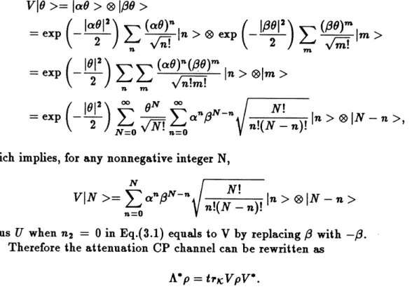
V from $\mathcal{H}$ to $\mathcal{H}\otimes \mathcal{K}$ as

$V|\theta>=|\alpha\theta>\otimes|\beta\theta>$ (3.6)

where $|\theta>represents$ a coherent vector $[4,8]$

.

$|\beta\theta>$

Fig. 4 Attenuation Process $V$

Now, _{let us show the equivalence of the above operator V and the operator} $U$ in

the conventional expression.

$V|\theta>=|\alpha\theta>\otimes|\beta\theta>$

$= \exp(-\frac{|\alpha\theta|^{2}}{2})\sum_{n}\frac{(\alpha\theta)^{\mathfrak{n}}}{\sqrt{n!}}|n>\otimes\exp(-\frac{|\beta\theta|^{2}}{2}I\sum_{m}\frac{(\beta\theta)^{m}}{\sqrt{m!}}|m>$

$= \exp(-\frac{|\theta|^{2}}{2})\sum_{n}\sum_{m}\frac{(\alpha\theta)^{n}(\beta\theta)^{m}}{\sqrt{n!m!}}|n>\otimes|m>$

which implies, for any

nonnegative integer

$N$

,

$V|N>= \sum_{n=0}^{N}\alpha^{n}\beta^{N-n}\sqrt{\frac{N!}{n!(N-n)!}}|n>\otimes|N-n>$

Thus $U$ when _{$n_{2}=0$} in Eq.(3.1) equals to V by replacing_{$\beta with-\beta$}

.

Therefore the attenuation CP channel can be rewritten as

$A^{*}\rho=tr\kappa V\rho V^{*}$

.

(3.7)

In this paper, we use this expression Eq.(3.7) to the derivation oferror

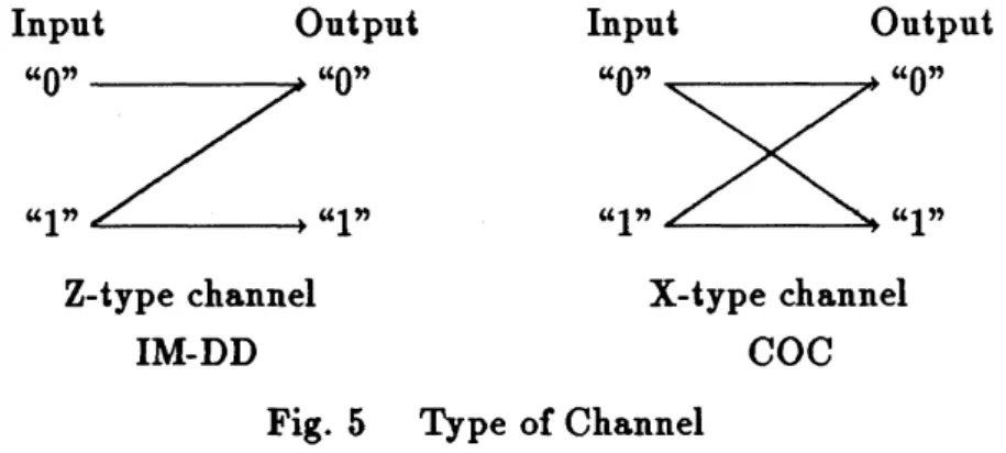
IV. QUANTUM CODING AND TYPES OF CHANNEL

In this section, before we derive concrete error probabilities, wereviewsome basic

facts for quantum coding and two types ofchanneling transformation.

Suppose that, by some procedure, we encode an information representing it by

a sequence of letters $c^{(1)},$

$\ldots$ ,$c^{(n)},$$\ldots$

,

where

$c^{(h)}$ is an element in a set $C$ of symbols

caUed the alphabet.

A quantum code is a map which associates to each symbol (or sequence of

sym-bols) in$C$a quantum state, representing anopticalsignal. Thisexpression is called the

quantum mechanical coding. Let $\rho$; be the quantum code corresponding to a symbol

$c;\in C$

.

We usuaUy take

$C=\{0,1\}\Leftrightarrow\Xi=\{\rho 0,\rho_{1}\}$

.

(4.1)

Then we assume that the noise state $\zeta\in 6(\mathcal{K}_{1})$ is a vacuum state due to the

“ _zero point _fluctuation ” _{ofelectromagnetic field. Therefore, when we derive error}

probabilities, we have to consider the following two types ofchannel : Z-type channel

and X-type channel. Each type of channel corresponds to IM-DD and COC,

respec-tively because the information associated to theinput state is set by different manners

in IM-DD and COC.

Input Output Input Output

Z-type channel X-type channel

IM-DD COC

Fig.

5

Type of Channel

At first, in the case of IM-DD, we usually take $\rho_{0}$ for the vacuum state and $\rho_{1}$

for another state such as a coherent state or a squeesed state. Since the noise state

₆

is a

vacuum

state, the input signal $u_{0’}$ represented by the state $\rho_{0}^{(1)}$

,

is error

&ee

in

the sense that it always

goes

to the output signal $0$ represented by $\rho_{0}^{(2)}$

,

while the

input signal 1, represented by the state $\rho_{1}^{(1)}$

,

is not error free in the sense that its

output may reach to both states$\rho_{0}^{(2)}$ and$\rho_{1}^{(2)}$ with different probabilities. We _$caU$ this

channel Z-type channel. Then the error probablity $P_{e}$ for IM-DD is given by

$P_{e}=P_{\epsilon 1}$ (4.2)

where $P_{e1}$ is the error probability that the signal 1 is read as the signal $0$

.

On the other hand, in the case of COC, the information is carried by amplitude,

frequency orphase of theinput state. Therefore, regardlessof thenoisestate$\zeta$

,

bothof

in the output system. We $caU$ this channel X-type channel. Here we assume the

input signals $0$ and

1

aretransmitted with equal probability 1/2, so that an error

probability $P_{e}$ for digital modulation is given by

$P_{e}= \frac{P_{e0}+P_{e1}}{2}$ (4.3)

where $P_{e0}$ and $P_{e1}$ are the error probabilities associated with the input signal $O’$and

the input signal 1’, respectively.

V. RJGOROUS DERIVATION OF ERROR PROBABILTY IN IM-DD

As discussed in [3], POVM (positive operator valued measure) is a useful tool to

describe quantum measurementprocesses. Therefore we apply theattenuationchannel

and each POVM expression to the derivation of error probabihty for a coherent input

state and a squeezed input state.

Direct detection is a measurement of photons in a transmitted state, so that the

POVM for the direct detection is given by

$E_{DD}(n)=|n><n|$ (5.1)

where

1

$n>is$ the n-th number photon vector in $?t_{2}$

.

In particular, in case of IM-DD, we consider only Z-type channel. That is, direct

detection in IM-DD measures the number of photons in the transmitted state and

decides whether the output state is vacuum or not.

Therefore, when the input state$\rho_{1}$ is transmitted to an output state $A^{*}(\rho_{1})$

,

the

general formula of the error probabi]ity $q_{e}$ that the state $A(\rho_{1})$ is recognized as a

vacuum state by mistake is given by :

$q_{\epsilon}=tr\uparrow t_{2}^{A}\rho_{1}E_{DD}(0)$

$=tr_{H_{2}^{tr_{\mathcal{K}_{2}^{V\rho_{1}V^{*}E_{DD}(0)}}}}$ (5.2)

A. PPM

In the case of PPM, since each symbol pulse is used for each quantum code, the

error probability $P_{e^{PPAf}}$ becomes

$P_{e}^{PPAf}=q_{e}$

.

(5.3)

1) _{Coherent state}

From Eq.(5.2) and Eq.(5.3), the error probability $P_{e(CO)}^{PPAf}$ for a coherent state

$\rho_{1}=|\theta><\theta|$ is given by

$q_{e}=tr_{\mathcal{H}_{2}}(tr_{\mathcal{K}_{2}^{V}}|\theta><\theta|V^{*})|0><0|$

$=tr_{\mathcal{H}_{2}}(tr_{\mathcal{K}_{2}}|\alpha\theta><\alpha\theta|\otimes|\beta\theta><\beta\theta|)|0><0|$

$=tr_{\mathcal{H}_{2}}|\alpha\theta><\alpha\theta||0><0|$

where $\eta=\alpha^{2}$ and $\eta$is constant describing thetransmission efficiency for the channel.

2)_{Soueezed state}

A squeezed state can be expressed by a unitary operator $U(z)(z\in C)$ such that

$\rho_{1}=U(z)|\theta><\theta|U(z)$

where $|\theta>is$acertain coherent vector. More concretely a squeezed vector $U(z)|\theta>$

is expressed as $[19,25]$

.

$U(z)|\theta>\equiv|\theta_{q}$ ; $\mu,$ $\nu>$ $b\equiv\mu a+\nu a$ $\theta=\mu\theta_{q}+\nu\overline{\theta_{\iota q}}$

$b|\theta_{q}$ ; $\mu,$ $\nu>=(\mu\theta_{q}+\nu\overline{\theta_{q}})|\theta_{q}$; $\mu,$ $\nu>$ $|\mu|^{2}-|\nu|^{2}=1$

$\mu=\cosh z$

$\nu=\exp(i\phi)\sinh z$

Then, from Eq.(5.2) and Eq.(5.3), the error probability $P_{e(SQ)}^{PPAf}$ for a squeezed state

$\rho_{1}=U(z)|\theta><\theta|U(z)$ is given by

$q_{\epsilon}=tr_{?t_{2}}(tr_{\mathcal{K}_{2}^{VU(Z)}}|\theta><\theta|U(z)^{*}V^{\cdot})|0><0|$

$=tr\mu_{1}U(z)|\theta><\theta|U(z)(V^{*}(|0><0|\otimes I)V)$

$=<U(z)\theta,$ $V^{\cdot}(|0><0|\otimes I)VU(z)\theta>$

$= \frac{1}{\pi^{2}}\int\int d^{2}vd^{2}w<U(z)\theta,$ _{$w><\alpha w,$ $0><\beta w,$} $\beta v>$

$\cross<0,$ $\alpha v><v,$ $U(z)\theta>$

This can be computed by the following

Gaussian

type

integration

:

$\frac{1}{\pi}\int d^{2}w\exp\{-|w|^{2}+aw+b\overline{w}+cw^{2}+d\overline{w}^{2}\}=\frac{1}{\sqrt{1-4cd}}\exp\{\frac{a^{2}d+ab+b^{2}c}{1-4cd}\}$

.

(5.5)

The result is

$q_{e}= \sqrt{\tau}\exp[\{(1-\eta)\tau-1\}|\theta|^{2}+\{1-(1-\eta)^{2}\tau\}\{\frac{\overline{\nu}\theta^{2}}{2\mu}+\frac{\nu\overline{\theta}^{2}}{2\overline{\mu}}\}]$ (5.6)

where $\tau=\{|\mu|^{2}-(1-\eta)^{2}|\nu|^{2}\}^{-1},$ $\mu$ and $\nu$ are complex numbers satisfying

1

$\mu|^{2}-|\nu|^{2}=1$

.

In the case that the code has the weight $N$ (the number of symbol 1), the

j-multiple error probability in the output system is

$P^{(j)}={}_{N}C_{j}i_{e}(1-q_{\epsilon})^{N-j}$

,

(5.7)

where

${}_{N}C_{j}= \frac{N!}{j!(N-j)!}$

Therefore, when the code with the weight $N$ is transmitted, the error probability

$P_{e^{PCAf}}$ for PCM modulation with $t_{0}$ -tuple error correcting code with the weight $N$ is

given by:

$P_{e}^{PCM}= \sum_{j=t_{0}+1}^{N}P^{(j)}$

$= \sum_{j=t_{0}+1}^{N}{}_{N}C_{j}\dot{\phi}_{e}(1-q_{e})^{N-j}$

.

(5.8)

By substituting Eq.(5.4) and Eq.(5.6) in the above formula Eq.(5.8), we can easily

compute the error probabilities $P_{e(CO)}^{PC1\psi}$ and $P_{\epsilon(SQ)}^{PCM}$

.

VI. RJGOROUS DERIVATION OF ERROR PROBABILTY

IN COHERENT OPTICAL COMMUNICATION

A. P.D.F.

_for

Each Detection

1)_{Homod ne Detection}

Homodyne detection is a measurement of the real part of the complex amlitude

ofa transmitted state. Therefore the P.O.V.M. $E_{HO}$ for homodyne detection is given

by

$E_{HO}( \Delta^{HO})=\int_{A^{HO}}|\theta_{x}><\theta_{x}|\mathscr{O}_{x}$ (6.1)

where $|\theta_{x}>$ is the

eigenvector

of the operator $a_{x}=(a+a^{*})/2$ and $a$ is the

annihilation operator of photon, $\Delta^{HO}$ is the set of real variables $\theta_{x}$

.

The infinitesimal

nonnegative

definite Hermitian operator $dE_{HO}(\theta.)$ is

given

by

$dE_{HO}(\theta_{x})=|\theta_{x}><\theta_{x}|d\theta_{x}$ (6.2)

The probability density function $p^{HO}(\theta_{x})$ ofthe outcomes is

$p^{HO}(\theta_{r})d\theta_{r}=tr_{?t_{2}^{A^{*}\rho dE_{HO}(\theta_{x})}}$

so that the probability density function $p^{HO}(\theta_{x})$ is

$p^{HO}(\theta_{x})=\iota_{r?t_{2}^{A^{\cdot}\rho}}|\theta_{x}><\theta_{x}|$ (6.3)

We derive the probabihty density function $p_{CO}^{HO}(\theta_{x})$ for a coherent input state.

$p_{CO}^{HO}(\theta_{x})=tr\uparrow t_{2}^{A(|}\theta><\theta|)|\theta_{g}><\theta_{x}|$ $=|<\theta_{x}|\alpha\theta>|^{2}$

$=\sqrt{\frac{2}{\pi}}\exp(-2(\theta_{x}-\alpha Re(\theta))^{2})$ (6.4)

This probability density function $p_{oO}^{HO}(\theta_{x})$is a Gaussian type. Then _{$m_{CO}$} and $\sigma co^{2}$

,

the average and the variance for this distribution$p_{CO}^{HO}(\theta_{x})$

,

are calculated as

$m_{CO}^{HO}=\alpha Re(\theta)$

,

$\sigma_{CO}^{HO^{2}}=\frac{1}{4}$ (6.5)

On

the otherhand, in thecaseofa squeezedinputstate, we derive theprobability

density function $p_{SQ}^{HO}$ from Eq.(6.3).

$p_{SQ}^{HO}(\theta_{x})=tr_{\mathcal{H}_{2}}(tr_{\mathcal{K}}(VU(z)|\theta><\theta|U(z)^{*}V^{*})|\theta_{x}><\theta_{x}|$

$=tr_{?t_{1}^{U(z)}}|\theta><\theta|U(z)(V^{\cdot}(|\theta_{x}><\theta_{x}|\otimes I)V)$

$= \frac{1}{\pi^{2}}\int\int d^{2}vd^{2}w<U(z)\theta,$ _{$w><\alpha w,$} $\theta_{a}><\beta w,$ $\beta v>$

$\cross<\theta_{a},$ _{$\alpha v><v,$ $U(z)\theta>$}

$= \frac{1}{\sqrt{2\pi\{\frac{1}{4}\eta|\mu-\nu|^{2}+\frac{1}{4}(1-\eta)\}}}\exp(-\frac{(\theta_{l}-\alpha Re((\overline{\mu}-\overline{\nu})\theta))^{2}}{2\{\frac{1}{4}\eta|\mu-\nu|^{2}+\frac{1}{4}(1-\eta)\}})(6.6)$

This probability density function $p_{SQ}^{HO}(\theta_{x})$ is

again

a Gaussian type. Then _{$m_{SQ}$} and

$\sigma_{SQ^{2}}$

,

the

average

and the variance ofthis distribution Eq.(6.6), are calculated as

$m_{SQ}^{HO}=\alpha Re((\overline{\mu}-\overline{\nu})\theta)$

,

$\sigma_{SQ}^{HO^{2}}=\frac{1}{4}\eta|\mu-\nu|^{2}+\frac{1}{4}(1-\eta)$

.

(6.7)

2)Heterod ne Detection

Heterodyne detection is a simultaneous measurement of the real and the

imagi-nary parts ofthe complex anlitude in a transmitted state. Therefore the heterodyne

detection may not depend on the effect of squeezing, so that we derive the error

probabilities for a coherent input state only.

Let $E_{HE}$ be the P.O.V.M. for heterodyne detection.

where

1

$\theta>is$ a coherent vector, and $\Delta^{HE}$ is the set ofcomplex variables $\theta$

.

Therefore the infinitesimal nonnegative definite Hermitian operator $dE_{HE}(\theta)$ is

given

by

$dE_{HE}( \theta)=|\theta><\theta|\frac{d^{2}\theta}{\pi}$ (6.9)

Thejoint probability density function $p^{HE}(\theta_{x}, \theta_{y})$ of the outcomes becomes

$p^{HE}(\theta_{x}, \theta_{y})d^{2}\theta=tr_{\mathcal{H}_{2}^{A\rho dE_{HE}(\theta)}}$

$= tr_{\mathcal{H}_{2}^{A\rho}}|\theta><\theta|\frac{d^{2}\theta}{\pi}$

so that thejoint probabihty density function $p^{HE}(\theta_{x}, \theta_{y})$ is :

$p^{HE}( \theta_{x}, \theta_{y})=\frac{1}{\pi}tr\mu_{2}A^{\cdot}\rho|\theta><\theta|$ (6.10)

For a coherent state $\rho=|\theta><\theta|,$ $p^{HE}(\theta_{x}, \theta_{y})$ is concretely derived as :

$p^{HE}(\theta_{x}, \theta_{y})=\underline{1}t_{I\mathcal{H}_{2}}A^{\cdot}\rho|\theta><\theta|$ $\pi$

$= \frac{1}{\pi}|<\theta|\alpha\theta_{S}>|^{2}$

$= \frac{1}{\pi}\exp(-|\theta-\alpha\theta_{S}|^{2})$ (6.11)

where the index $s$ represents the signal $0$’ or 1’.

Then the coherent detection demodulate the part $\cos$wt” bom the transmitted

signal. We let $pH^{E}(\theta.)$ the marginal probability density function of$p^{HE}(\theta_{x}, \theta_{y})$

,

and

from Eq.(6.11) $p_{co}^{HE}(\theta_{x})$is given by

$p_{co}^{HE}( \theta_{x})==\frac{\int_{1}p}{\sqrt{\pi}}\exp(-t^{\nu_{\theta_{l}-\alpha Re(\theta_{S}))^{2})}}HE(\theta_{l},\theta)d\theta_{y}$

.

(6.12)

This probability density function $p_{co}^{HE}(\theta_{x})$ is also a Gaussian type. Then $m_{co}^{HE}$ and

$\sigma_{co}^{HE^{2}}$

,

the

average

and the variance ofthis distribution Eq.(6.12),

are calculated as

$m_{co}^{HE}=\alpha Re(\theta_{\iota})$

,

$\sigma_{co}^{HE^{2}}=\frac{1}{2}$ (6.13)

On the other hand, the envelope detection [18] demodulates the envelope of the

transmitted signal. Let $g(r)$ be the probability density function for the envelope

detection. It is well known that we can get the following probability density function

$g(r)$ from Eq.(6.11):

where$I_{0}$is the zeroth-order modified Bessel function of the first kind. The distribution

$g(r)$ in Eq.(6.14) is caUed a Rice distribution [18].

B. $OOK$ Homodyne Detection

In OOK, $\rho_{0}$ is a vaccum state and $\rho_{1}$ is another state such as a coherent state

and a squeezed state in the input system $?t_{1}$

.

1) Coherent state

The probability density functions $p_{0(CO)}^{HO}(\theta_{x})$ and $p_{1(CO)}^{HO}(\theta_{x})$ for the signal $0$’

and 1’ are respectively obtained by Eq.(6.4) as

$p_{0(CO)}^{HO}(\theta_{x})=\sqrt{\frac{2}{\pi}}\exp(-2\theta_{l}^{2})$ (6.15)

$p_{1(CO)}^{HO}(\theta_{x})=\sqrt{\frac{2}{\pi}}\exp(-2(\theta_{x}-\alpha Re(\theta_{1}))^{2})$ (6.16)

Every error probability of

OOK

for each signal turns to be identical. That is,

$P_{\epsilon 0(CO)}^{OOK-HO}=P_{e1(CO)}^{OOK-HO}= \int_{\alpha Re(\theta_{1})/2}^{\infty}p_{0(CO)}^{HO}(\theta_{x})d\theta_{x}$ (6.17)

Hence the error probabihty $P_{\epsilon(CO)}^{OOK-HO}$ is

given

by

$P_{e(CO)}^{OOK-HO}= \frac{1}{2}$erfc $( \frac{\sqrt{\eta}Re(\theta_{1})}{\sqrt{2}})$

,

(6.18)

where erfc(x) is the complementary error function given by

erfc(z) $= \frac{2}{\sqrt{\pi}}l^{\infty}\exp(-t^{2})dt$ (6.19)

2)Squeezed _state

Under the similar discussion as the case ofa coherent state, the error probability

is

given

by

$P_{e(SQ)}^{OOK-HO}= \frac{1}{2}$ erfc $( \frac{\sqrt{\eta}Re((\overline{\mu}-\overline{\nu})\theta_{1})}{\sqrt{2\eta|\mu-\nu|^{2}+2(1-\eta)}})$ (6.20)

C. BPSKHomodyne Detection

In BPSK, $\rho_{0}$ is a state with the phase $0$ and $\rho_{1}$ is a state with the phase $\pi$

.

The probability density functions $p_{0(CO)}^{HO}(\theta_{x})$ and $p_{1(OO)}^{HO}(\theta_{x})$ for the signal $0$

and 1 are respectively obtained from Eq.(6.4).

$p_{0(CO)}^{HO}(\theta_{r})=\sqrt{\frac{2}{\pi}}\exp(-2(\theta_{a}-\alpha|\theta|)^{2})$ (6.21) $p_{1(CO)}^{HO}(\theta_{x})=\sqrt{\frac{2}{\pi}}\exp(-2(\theta_{x}+\alpha|\theta|)^{2})$ (6.22)

where

1

$\theta|$ is the amplitude in an input state $\rho 0$ or$\rho_{1}$

.

We obtain the error probability for BPSK

$P_{e0(GO)}^{EPSK-HO}=P_{e1(CO)}^{BPSK-HO}= \int_{0}^{\infty}p_{1(CO)}^{HO}(\theta_{x})d\theta_{x}$ (6.2$)

Then the error probability $P_{e(CO)}^{BPSK-HO}$ is given by

$P_{\epsilon(CO)}^{BPSK-HO}= \frac{1}{2}$erfc$(\sqrt{2\eta}|\theta|)$ (6.24)

2)

_Soueezed

_state

Under the similar discussion as the case of acoherent state, the error probability

is given by

$P_{e(SQ)}^{BPSK-HO}= \frac{1}{2}$erfc $( \frac{\sqrt{2\eta}|\theta|Re(\overline{\mu}-\overline{\nu})}{\sqrt{\eta|\mu-\nu|^{2}+(1-\eta)}})$ (6.25)

D. $OOK$ Heterodyne Coherent Detection

From Eq.(6.12) the probability density functions $p_{0(CO)}^{HE}(\theta_{x})$ and $p_{1(CO)}^{HE}(\theta_{x})$ for

the signal $0$ and 1’ are respectively given by

$p_{0(OO)}^{HE}( \theta_{x})=\frac{1}{\sqrt{\pi}}\exp(-\theta_{r}^{2})$ (6.26)

$p_{1(CO)}^{HE}( \theta_{x})=\frac{1}{\sqrt{\pi}}\exp$($-(\theta_{x}$ –a$Re(\theta_{1})$) ) (6.27)

As is analogized from the case OOK-homodyne, the error probability $P_{e(CO)}^{OOK}$ is

given by

$P_{e(CO)^{-HE}}^{OOK}= \frac{1}{2}$ erfc $( \frac{\sqrt{\eta}Re(\theta_{1})}{2})$ (6.28)

E. $OOK$ Heterodyne Envelope Detection

From Eq.(6.14) the probability density functions $g_{0}(r)$ and $g_{1}(r)$ for the signal

$0$’ and 1 are respectively given by

$g_{0}(r)=2r\exp(-r^{2})$ (6.29)

Therefore, by a proper approximation given in [18], the error probabihty $P_{e(EN)}^{OOK}$

becomes :

$P_{\epsilon(EN)^{-HE}}^{OOK}= \frac{1}{2}\exp(-\frac{\eta|\theta_{1}|^{2}}{4}I$ (6.31)

F. $FSK$ Heterodyne

Cohere

$nt$ Detection

In FSK, $\rho_{0}$ is a state with the frequency $w_{0}$ and $\rho_{1}$ is a state with $w_{1}$

.

The

transmitted state $A^{\cdot}\rho_{0}$ or $A^{\cdot}\rho_{1}$ is separated by IF(intermediate frequency) dual filter

and demodulated by coherent detectors [18]. Here we can consider only the case that

the signal $0$“ is transmitted without loss of genenality. Let A and $B$ be the above

two coherent detectors, and let $\theta_{A}$ and $\theta_{B}$ be each outcome of A and $B$, respectively.

From Eq.(6.12), the probability density functions $p_{A(CO)}^{HE}(\theta_{A})$ and$p_{B(CO)}^{HE}(\theta_{B})$ for the

outcomes ofA and $B$ are respectively

given

by

$p_{A(CO)}^{HE}( \theta_{A})=\frac{1}{\sqrt{\pi}}\exp(-(\theta_{A}-\alpha Re(\theta_{0}))^{2})$ (6.32)

$p_{B(CO)}^{HE}( \theta_{B})=\frac{1}{\sqrt{\pi}}\exp(-\theta_{B}^{2})$ (6.3$)

The error probability $P_{e(CO)}^{FSK}$ is given by

$P^{FSK-HE}=$ _Prob$(\theta_{A}-\theta_{B}<0)$

$e(CO)$

$= \int_{-\infty}^{0}\frac{1}{\sqrt{2\pi}}\exp(-\frac{(\theta_{A-B}-\alpha Re(\theta_{0}))}{2})d\theta_{A-B}$

$= \frac{1}{2}$ erfc $( \frac{\sqrt{\eta}Re(\theta_{0})}{\sqrt{2}})$ (6.34)

where $\theta_{A-B}=\theta_{A}-\theta_{B}$

.

G.

$FSK$Heterodyne Envelope Detection

Here, we consider the case without loss ofgenerality that the signal 1’is

trans-mitted. From Eq.(6.14) the probability density functions $g_{A}(r)$ and $g_{B}(r)$ for the

outcomes ofthe band pass filter A and $B$’ are respectively given by

$g_{A}(r_{A})=2rA\exp(-\gamma_{A}^{2})$ (6.35)

$g_{B}(r_{B})=2tB\exp(-r_{B}^{2}-|\alpha\theta_{1}|)I_{0}(2r_{B}|\alpha\theta_{1}|)$ (6.36)

Whenever $r_{A}>r_{B}$

,

an error occurs. Thus we can get the following formula

$P_{e(EN)}^{FSK-HE}= \int_{B}^{\infty_{=0}}g_{B}(r_{B})(\int_{4B}^{\infty_{=}}g_{A}(r_{A})d\prime_{A)}dr_{B}$

where we applied the approximation given in [18] to this derivation.

H. BPSK Heterodyne Coherent Detection

From Eq.(6.12) the probability density functions $p_{0(CO)}^{HE}(\theta_{x})$ and $p_{1(CO)}^{HE}(\theta_{x})$ for

the signal $0$’ and 1 are respectively given by

$p_{\mathfrak{U}^{E}}^{H_{CO)}}(\theta_{x})=\sqrt{\frac{1}{\pi}}\exp(-(\theta_{x}-\alpha|\theta|)^{2})$ (6.38)

$p_{1(CO)}^{HE}(\theta_{x})=\sqrt{\frac{1}{\pi}}\exp(-(\theta_{x}+\alpha|\theta|)^{2})$ (6.39)

where $|\theta|$ is the amplitude in an input state $\rho_{0}$ or $\rho_{1}$

.

Byananalogyof thecase inBPSK-Homodyne, the errorprobability $P_{e(CO)}^{BPSK}$

is

given

by

$P_{e(CO)}^{BPSK-HE}= \frac{1}{2}$erfc$(\sqrt{\eta}|\theta )$ (6.40)

I. BPSKHeterodyne

_Differential

Detection

This systemisoftencaUed “DPSK”. The informationisrepresented by thechange

of phase between two successive signals. Therefore the signal is demodulated by the

product of two successive outcomes, that is, the signal is recognized as $0$’ when the

product is positive and the signal is recognized as $0$ when the product is negative.

Then the error probability $P_{e^{DPSK}}$ is given by

$P_{e}^{DPSK-HE}= \frac{1}{2}\exp(-\eta|\theta, |^{2})$ (6.41)

using some results obtained in [18].

VII. NUMERICAL RESULTS

Fig.7 shows that each error probability for PPM is smaUer than that for

PCM

at any transmission efficiency $\eta$

.

In this simulation, PCM does not have any

error-corrections, however, if

PCM

has some error-correction, then the relation between

them may be opposite to this result. On the other hand, this result tells us that the

stronger the effect ofsqueezingbecomes, the better the efficiency becomes. However, in

thecase of IM-DD, the informationis represented by the number of photons contained

in each pulse. Therefore it is generaUy difficult to examine the effect ofsqueezing for

the parameter $\theta_{l}$

.

The comparison between

PCM

and PPM has been already well

discussed in our previous paper [14].

Next, let us discuss the efficiency about

COC

for a coherent input state and a

squeezed input state.

In the case that an input state is a coherent state, the results of Fig.8 has the

same relation with the numericalresultsin [24]. But our derivation is entirely different

$\underline{\sim_{\frac{o}{o}}\circ b}^{*}$ $\underline{Q_{\circ^{\frac{o}{u)}}}^{*}\backslash }$ $\ddot{A^{O}B\circ\circ\triangleleft}\succ$ $\mathfrak{g}^{\circ}’.rbo\circ\alpha$ $\triangleright^{\circ}b_{?}$ $g^{\dot{\circ}}8_{?}$

$\prime 1^{\backslash }ransn\iota$issionElficiency

$\eta$ Transmission Efficiency$\eta$

Fig.7 Error probabilityforIM-DD Fig.8 Errorprobability foreachcoherent state

$\underline{Q_{\circ^{\frac{o}{0}}}b;}$ $\underline{O_{b^{\frac{\neg 0}{o^{\mathfrak{d}}}}}}$ $\frac{\succ}{\dot{m}^{\circ}A_{\circ}^{d_{\supset}}.}$ $\frac{\sim}{..:=\circ,\alpha}$ $\circ\dot{L}\circ$ $r\dot{\triangleleft}\circ$ $f^{\dot{\circ}}d8$

Transmission EfTiciency$\eta$

TransmissionEfficiency$\eta$

$\underline{o_{o^{\backslash }}}\frac{o}{\omega}$ $\underline{Q_{\circ^{\frac{o}{0}}}b^{\backslash }}$

$\dot{[be]}^{=}p_{\circ}r_{d}g\circ$ $\dot{[be]}^{o^{6}}\prime r_{O}\circ=i\neg$

$\triangleright^{\dot{\circ}}b_{J}$ $\triangleright^{\dot{\circ}}b_{3}$

TransmissionEfficiency $\eta$

TransmissionEMciency $\eta$

Fig.11 Error probability forOOKdirectdetection Fig.12 Errorprobsbihty forOOKhomodynedetection

$\underline{O_{b^{\frac{\backslash 0}{o^{0}}}}}$ $\underline{Q_{\circ^{\frac{o}{u)}}}\backslash }$ $\frac{\approx}{.}\circ\dot{L}\grave{\circ}\circ$’ $”’\dot{L}\circ\circ=\circ\triangleleft\approx$ $\triangleright^{\dot{\circ}}b_{J}$ $\dot{\omega^{\vee}}\dot{\circ}$

Transmission$Elfi$ciency$\eta$

Transmission$C^{}$Ificiency

$\eta$

error probabihty for a squeezed input state $[15,16]$

.

The relation

among

modulation,

detection and demodulation are given by the following (Fig.8):

modulation : $P_{e}^{BPSK}\leqq P_{\epsilon}^{FSK}\leqq P_{e}^{OOK}$

detection : $P_{e}^{Homodpn\epsilon}\leqq P_{\epsilon}^{H\epsilon t\epsilon odyne},$$P_{\epsilon}^{Di\epsilon c}$

demodulation : $P_{\epsilon}^{Coh\epsilon\prime\epsilon nt}\leqq P_{\epsilon}^{Diffe}$ $\leqq P_{e}^{Envelop\epsilon}$

In particular, concerning the detection, it is obvious that the efficiency for homodyne

dection is better than that for heterodyne detection because the quantum limits on

the homodyne detection is smaUer. However we can not compare the efficiency for

heterodyne detection and direct detection quantitatively, because the obsevable for

these detections are different

&om

each other.

As we see in Fig.8, the efficiency for BPSK with homodyne detection is the best

of $aU$

.

Therefore, in thi$s$ paper, we consider this ultimate efficiency for BPSK with

homodyne detection, that is, that for a squeezed input state.

In order to study the efficiency for a squeezd input state, we consider two cases

for the first setting. One case is that the average number of photons in a coherent

state before

squeezing

is fixed (Fig.9-11). The other case is that the

average

number

of photons in a squuezed state is fixed (Fig.12-14).

From Fig.9-11, we have

$P_{e}(16:1)\leqq P_{\epsilon}(4:1)\leqq P_{\epsilon}(1 : 1)\leqq P_{\epsilon}(1 : 4)\leqq P_{e}(1$ :

16

$)$ (7.1)

On the contrary, from Fig.12-14, we have

$P_{\epsilon}(1 : 16)\leqq P_{e}(1 : 4)\leqq P_{e}(1 : 1)\leqq P_{e}(4:1)\leqq P_{e}(16:1)$ (7.2)

Let us consider the reason why we got the above inequalities. In the former case

(Fig.9-11), thesqueezing is not effective for the attenuationcommunication processes.

Moreover this result is just opposite to the result expected. This is because the

coherent state loses the energy for squeezing if the number of photons in a coherent

state before

squeezing

is fixed. In the case of $\sigma_{r}$ : $\sigma_{l}=1$ :

16

for squeezing the

parameter $\theta_{a}$

,

we need the highest

energy

of$aU$ cases above. Here we examine the

result by changing a squeezed input state in the attenuation processes. We derive the

probability density function $p_{SQ}^{HO}$ for an

imarginary

part $\theta_{y}$ of a complex amplitude as

same as Eq.(6.6)

$p_{SQ}^{HO}(\theta_{y})=tr_{\mathcal{H}}(tr_{\mathcal{K}}(VU(z)|\theta><\theta|U(z)^{*}V^{*})|\theta_{y}><\theta_{y}|$

$=tr_{\mathcal{H}_{1}^{U(z)}}|\theta><\theta|U(z)(V^{\cdot}(|\theta_{r}><\theta_{y}|\otimes I)V)$

$= \frac{1}{\pi^{2}}\int\int d^{2}vd^{2}w<U(z)\theta,$ _{$w><\alpha w,$} $\theta_{y}><\beta w,$ $\beta v>$

$\cross<\theta_{\bullet},$ _{$\alpha v><v,$ $U(z)\theta>$}

This probabihty density function $p_{SQ}^{HO}(\theta_{y})$ is

again

a Gaussian type. Then $m_{SQ}’$ and

$\sigma_{SQ}^{\prime 2}$

,

the

average

and the variance ofthis distribution Eq.(7.3), are calculated as

$m_{SQ}’=\alpha Re((\overline{\mu}+\overline{\nu})\theta)$, $\sigma_{SQ}^{\prime 2}=\frac{1}{4}\eta|\mu+\nu|^{2}+\frac{1}{4}(1-\eta)$

.

(7.4)

Therefore, from Eq.(6.7) and Eq.(7.4), the variance ofeach part of a complex

ampli-tude for a squeezed state in the attenuation processes is given by:

$\{\begin{array}{l}\sigma_{l}^{2}=\frac{1}{4}\eta|\mu-\nu|^{2}+\frac{1}{4}(1-\eta)\sigma_{l}^{2}=\frac{1}{4}\eta|\mu+\nu|^{2}+\frac{1}{4}(1-\eta)\end{array}$

This implies that a squeezed state in the attenuation processes is not a minimum

uncertainty state. Thatis, theeffect ofsqueezing is losing inthe attenuationprocesses.

On the other hand, if the number of photons in a squeezed state is fixed, the

squeezing is effective for the optical communication. In this case we have only to

consider the loss of

energy

in the attenuation processes, which is shown in Fig.9-14.

One of further discussionsis to find the optimal method for use of a squeezed state in

the optical communications [16].

This paper totally studied rigorous mathematical expressions for quantum

com-municationprocessesandapplied them to derivevarious error probabilitiesinageneral

standing point. This rigorous and general theory contains most ofthe results shown

by many authors such as Yuen and Shapiro [26,27,28].

IX. REFERENCES

[1] L. Accardi and M. Ohya, “Compoud channels, transition expectations and

lift-ings”, to appear in J. Multivariate Anal.

[2] C.M. Caves, “Quantum limits on noise in linear amplifiers“, Phys.Rev.$D$

,

Vo1.26,

pp.1817-1839 (1980).

[3] E.B. Davies, “Quantum Theory ofOpen Systems”, Academic Press (1976).

[4] R.J. Glauber, “Coherent and incoherent statesofthe radiation field”, Phys. Rev.

Vol.131, pp.2766-2788 (1963).

[5]

C.W.

Helstrom, “Quantum

Detection

and Estimation Theory”, Academic Press

(1976).

[6] O. Hirota, “Optical Communication Theory”, Morikita Publishing (1985).

[7] A.N. Kolmogorov, “On the representation ofcontinuous functions of many

vari-ables by superpositionsofcontinuous functions one variable and addition”, Dokl.

Akad. Nauk, Vol.114, pp.679-681 (1957).

[8] W. Louisell, “Quantum Statistical Properties of Radiation”, Wiley (1973).

[9] M. Ohya, “Quantum ergodic channels in operator algebras”,J.Math.Anal.Appl.,

Vol.84, pp.318-327 (1981).

[10] M. Ohya, “On compound state and mutual information in quantum information

[11] M. Ohya, H. Yoshimi and O. Hirota, “Rigorous derivation of error probability

in quantum control communication processes“, IEICE of Japan, J71-B, No.4,

533-539

(1988).

[12] M. Ohya, “Some aspects of quantum information theory and their applications

to irreversible processes”, Rep. on Math. Phys., Vol.27, pp.19-47 (1989).

[13] M.Ohya, “Information dynamics and its applications to optical

communication-processes”, Springer Lec. Notes in Physics., Vol.378, pp.81-92 (1991).

[14] M. Ohya and H. Suyari, “optimization of error probability in quantum control

communication processes”, IEICE of Japan, J73-B-I, No.3,

200-207

(1990).

[15] M.Ohya and H.Suyari, “Rigorous derivation oferror probabihty in coherent

opti-cal communication”, Springer Lec. Notesin Physics., Vol.378, pp.203-212 (1991).

[16] M.Ohya and H.Suyari, “A mathematical study for optical communication

pro-cesses”, in preparation.

[17] C.E. Shannon, “A mathematical theory of communication”, Bell System Tech.J.,

Vol.27, pp.379-423,623-656 (1948).

[18] S. Stein andJJ. Jones, “Modern Communication Principles”, McGraw Hill, New

York (1965).

[19] D. Stoler, “Equivalence class ofminimum uncertainty packets”, Phys. Rev., Dl,

pp.3217-3219 (1970) and D4, pp.1925-1926 (1971).

[20] H. Takahashi, “Information theory of quantum mechanical channels“, Advances

in

Communication

Systems, Vol.1, Academic Press, pp.227-310 (1966).

[21] H. Umegaki and M. Ohya, “Entropies in Probabilistic Systems (in Japanese)”,

Kyoritsu Publishing (1983).

[22] H. Umegaki and M. Ohya, “Quantum Mechanical Entropies (in Japanese)”,

Ky-oritsu Publishing (1984).

[23] N. Watanabe, “Efficiency of optical modulations with coherent state”, Springer

Lec. Notes in Physics., Vol.378, pp.350-360 (1991).

[24] Y. Yamamoto,

”Receiver

performance evaluation of various digitaloptical

modu-lation-demodulation systems in the

0.5-1.0

$\mu m$ wavelength region”, IEEE.J.

Quantum Electron., QE-16, No.11, pp.1251-1259 (1980).

[25] H.P. Yuen, “Two-photon coherent states of the radiation field”, Phys. Rev., A13,

pp.2226-2243 (1976).

[26] H.P. Yuen and J.H. Shapiro, “Optical communication with two-photon

coher-ent states-Part I : Quantum state propagation and quantum noise reduction“,

IEEE.TransJnf.Theory, IT-24, No.6, pp.657-668 (1978).

[27] H.P. Yuen, J.H. Shapiro and J.A. Machado Mata, “Optical communication with

two-photon coherent states-Part II: Photoemissive detection and structured

re-ceiver performance”, IEEE.Trans.$Inf$.Theory, IT-25, No.2, pp.179-192 (1979).

[28] H.P. Yuen and J.H. Shapiro, “Optical communication with two-photon coherent

states-Part III : Quantum measurements realizable with photoemissive