When is a Stokes Line not a Stokes Line? : III. Real Consequences of the Higher Order Stokes Phenomenon (Recent Trends in Exponential Asymptotics)

C.J.Howls

University ofSouthampton

November 30,

2004

1

Introduction

Rom all the examples of theactivity ofStokeslines in the previoustwo papers Howts (2005ab),

the reader may be left with the impression that the higher order Stokes phenomenon is an

analyticalrelic whose influence isconfined to the complex plane. Inthis paper wedem onstrate

that thisisfar fromtrue,and that thehigherorder Stokesphenomenoncanresult in farreaching

effects in real space.

Here we shallstudytwo pedagogical examples. The firstis alinearpartial differentialequation

similar tothat ofthe second paper Howls (2005b). Hereweshall show that the activity ofStokes

lineshasboth aqualitative and quantitative effect onthe largetimebehaviour ofthesolution.

The second examples is Burgers equation. Although an integrable nonlinear PDEwe study it

because ofits canonical rolein the discussionofsmoothed shockwave form ation. We shall see

that when viewed from an asymptotic problem, thehigher order Stokes phenomenon iscrucial

to the mechanism for theformation of the shock.

2

Example: Linear Partial

Differential

Equation

We study the effect of the higher order Stokes phenomenonon the large time behaviour ofthe

partialdifferential system $-\infty<x<+\infty,$ $t>0$,

$u_{t}-u_{x}= \epsilon^{2}u_{\sigma ixx}-\frac{1}{1+x^{2}}$, $u(x, \mathrm{O})=\arctan x$, (2. 1)

where $u_{x},$ $u_{xx},$ $u_{xxx}arrow 0$ as $|x|arrow$ oo and $0<\epsilon<<1$

.

This system is intimately related to the

Howls et at (2004). However here, for ease, we shall use an integral approach to $\mathrm{i}1^{1}[perp] \mathrm{u}\mathrm{s}\mathrm{t}\mathrm{r}\mathrm{a}\mathrm{t}\mathrm{e}$

the

how thehigherorder Stokesphenomenonaffects theremainderterms andexpansionsin different

regions of the real a$=(x, t)$ plane.

The systemcan be solvedexactly by Fourier transformsas asumofintegrals

$u(x, t; \epsilon)=\arctan x+\sum_{j=1}^{2}I_{j}(x, t;\epsilon)+\sum_{j=3}^{4}I_{j}(x;\epsilon)$, (2.2)

where

$I_{1}(x, t; \epsilon)=\oint_{0}^{\infty}\frac{\mathrm{i}p/2}{p^{2}-1}e^{-f(p;x,t)/\epsilon}dp=I_{2}^{*}(x,t;\epsilon)$ , (2.3)

$I_{3}(_{X\mathrm{i}} \epsilon)=\oint_{0}^{\infty}\frac{\mathrm{i}p/2}{1-p^{2}}e^{-p(1+ix)/\epsilon}dp=I_{4}^{*}(x;\epsilon)$ , (2.4)

and

$f(p;x, t)=p(1+\mathrm{i}x)+\mathrm{i}p(1-p^{2})t$, (2.5)

The star denotes complex conjugation. In $I_{1}$ and

I3

(respectively

I2

and $I_{4}$) the contours are

indented around thepolesat$p=+1$inprescribedmannersuchthat there is(initially)nooverail

pole contribution andthe initial conditions

are

satisfied as $|x|arrow\infty$

For$t>0$, asymptoticcontributionsto $I_{1}$ and $I_{2}$ canarise from the endpointsat$p=0$, thepole

at$p=+1$, and oneoftwo saddlepoints. For$I_{3}$ and I4, analogous contributions

can

onlyarise

from theendpoint and thepole at$p=+1$

.

To studythe time evolutionm of the problemin the real $(x, t)$ plane, without loss ofgenerality

we

can

restrict our attentionto $I_{1}$.

The endpoint at $p=0$, isdenoted by thesuperscript/subscripts $e$; the pole $\mathrm{a}\mathrm{t} +1$ by

$p_{1}$, at $- 1$

by$p_{2}$; the saddies at

$p=\pm\sqrt{\frac{1}{3it}(1+\mathrm{i}(x+t))}$ _(2.6)

by $s_{1}$ (for $+$) and 82 (for $-$). The choice of notation is now seen to agree with the labelling

ofcontributions inthe second paper (Howls 2005b) allowingfor the additional terms that arise

from the sumof complex conjugates.

As weusethe integralrepresentationsit isquiteeasyto

see

nowthat theasymptoticbehaviours

are given by:

$e^{-f\mathrm{j}/\epsilon}T^{(g)}(\epsilon)$ (2.7)

where$j$denotes $e,$$s_{1}$ or$p_{1}$, with the following expressions

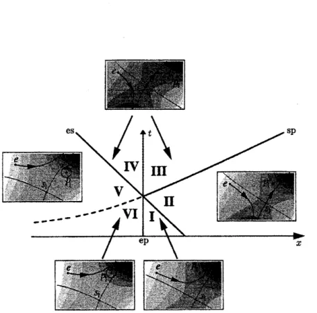
Figure 1: The sixregionsin the real$(x, t>0)$half-planeinwhich differentasymptoticbehaviours

for$I_{1}$

are

possible. TheseregionsaredeliniatedbyStokes lines. The notation “es”,forexample,

referstoanendpoint switching

on a

saddle contribution. The dashedStokeslinebetween$\mathrm{V}$ and

VI is active, but irrelevant. The dotted line between regions III andIV is an inactive Stokes

line.

$f_{s_{1}}(x, t)= \frac{2\mathrm{i}(x+t-\mathrm{i})^{3/2}}{3\sqrt{3t}}$, $T^{(\epsilon_{1})}(\epsilon;x,$$\mathrm{A}\sim\sum_{r=0}^{\infty}T_{r}^{(e_{1})}\epsilon^{r+1/2}$, (2.9)

$f_{\mathrm{P}1}(x, t)=1+\mathrm{i}x$, $T^{(\mathrm{p}_{1})}( \epsilon;x, t)=-\frac{1}{2}\pi$

.

(2.10)

The first coefficient of the saddlepointexpansion about $s_{1}$ is

$T_{0}^{(s_{1})}= \frac{1}{2}\mathrm{i}\sqrt{\pi i}\frac{(3t)^{1/4}(x+t-\mathrm{i})^{1/4}}{x-2t-\mathrm{i}}$

.

(2.11)

It is important tonote that contributions from thesaddle and endpoint

are

both (asymptotic)

infinite series. The single term contribution from the pole is exact.

Theconjugacyof$I_{2}$ and$I_{1}$

mean

thattheyhave analytically similar structures and the relevant

expansions

are

just the correspondingconjugates of (4.8). The contributions bom integral $I_{3}$

can

be obtained by setting $t=0$ in (2.9) and (2.10), and multiplying the results by-l. The

corresponding expansions for

_I4

are

the conjugates of those from

I3.

With all the above contributions it isastraightforward task to draw the candidate Stokes

curves

There arethree candidatesfor Stokes

curves:

.

the line$x=0$where

$F_{ep1}(x, t)\equiv f_{\mathrm{P}1}-f_{e}=1+\mathrm{i}x>0$ (2.12)

the endpoint may switch on

a

pole (residue) contribution;

.

along acurverunningforward in time from negative $x$ to positive $x$where

$F_{\mathrm{s}_{1}p_{1}}(x, t)\equiv$ $f_{p1}-f_{s_{\mathrm{I}}}=1+ \mathrm{i}x-2\mathrm{i}\frac{(x+t-\mathrm{i})^{3/2}}{3\sqrt{3t}}>0$ (2.13)

asaddle may switchon apole contribution;

.

alongthe line $x\mathrm{B}$$=1/\sqrt{3}$runningforward in time where

$F_{es_{1}}(x, t) \equiv f_{s_{1}}-f_{e}=2\mathrm{i}.\frac{(x+t-\mathrm{i})^{3/2}}{\mathrm{q}\sqrt{3t}}>0$, (2.14)

theendpoint may switch on a saddle.

Ananalysisofasequenceofplots of thesteepest descent contours as afunction of$x$ and$t$Jeads

to the findingsof figure 2. Theendpoint $e$contributes for all values of$x$ and $t$.

In region $\mathrm{I}$, only the endpoint

term contributes. Across the Stokes line between regions I

and $\mathrm{I}\mathrm{I}$, the dom inant endpoint switches on

a subdominant contribution from $s_{1}$. Across the

Stokescurvebetweenregions IIandIII, $s_{1}$ switcheson a (reiatively) subdominant contribution

from $p_{1}$ (which in turn is sub-subdominant to the contribution from $e$. Crossing $x=0$ from

region Iclockwise into region$\mathrm{V}\mathrm{I},$ $e$switcheson asubdominantpolecontribution from

$p_{1}$

.

This

combination persists across the apparent Stokes line between $s_{1}$, pi and into region $\mathrm{V}$, since

there is no $s_{1}$ yet present to switch $\mathrm{o}\mathrm{n}/0\mathrm{f}\mathrm{f}$

a

contribution from

$p_{1}$. Across the line between$\mathrm{V}$

arrd $\mathrm{I}\mathrm{V},$ $s_{1}$ is finally switchedon by $e$

.

Thus thereare contributions from _$e,$ $s_{1}$ and $p_{1}$ inboth

regions III and$\mathrm{I}\mathrm{V}$.

From (2.12) the axis along$x=0,$ $t>1/\sqrt{3}$ delineating regions III and IV should bea _Stokes

curve where a dominant $e$ switches on or off a subdominant contribution from

$p_{1}$

.

However,

the presence ofsuch aStokes curve would lead to a contradiction. For example, by continuing

from region III anti-clockwise to IV, $e$ should then switch off

$p_{1}$ so that no contribution from $p_{1}$ existed in $\mathrm{I}\mathrm{V}$. To the contrary,

the clockwise continuation around $t=1/\sqrt{3}$ from region I

suggests that IV should indeed contain

a

$p_{1}$ contribution. The conclusion is that despite the

presence ofthe _{necessary dominant and subdominant} terms, no Stokes phenomenon can take

place. This is confirmed bya steepest descent analysis (seeinsets in figure 1).

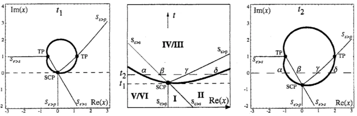
Thispictureisentirely consistentwith the Stokescurvegeometryplotted for areal$\mathrm{t}$-sectionin

Figure 2: The Stokes curves (solid lines) and the higher order Stokes

curve

(bold line) for $I_{1}$

(centre pane) compared with real sections complex $x$-planes (left and right panes) at times

$t=t_{1}=1/\sqrt{3}$ (dotted line in middle pane) and $t=t_{2}>1/\sqrt{3}$ (dashed line in middle pane).

Only the active and relevant Stokes

curves

have been drawn. The kidney-shaped higher order

Stokes

curve

growsinsizefrom$t=0^{+}$ andfirst intersectsreal $(x, t)$space at $t=t_{1}=1/\sqrt{3}$, the

minimum of the higher order Stokes

curve

in real $(x, t)$ space. Thereafter the Stokes curve $S_{ep}$

isinactive. The points$\alpha,$$\beta,$$\gamma,$$\delta$indicate the intersections of the Stokes andhigher order Stokes

curvesat $t_{2}$ (right pane) with the real$(x, t)$ plane (centrepane).

Stokes line in the complex $x$-plane does not intersect the real $(x, t)$ plane. The Stakes curve

$S_{e>\mathrm{p}}$ is active for $\Im(x)$ below the SCP but inactive above the higher order Stokes

curve.

As $t$ evolves between $0^{+}$ and $1/\sqrt{3}$ theintersection of the active $S_{e>p}$ curve traces out the active

Stokesline delineatingregions I and$\mathrm{V}\mathrm{I}$. At $t=1/\sqrt{3}$the SCP intersects with real $(x, t)$ plane

at $(0, 1/\sqrt{3})$ and switches offthe

curve

delineating regions IIIand$\mathrm{I}\mathrm{V}$. The curves delineating

IIandIII, IV and$\mathrm{V}$ respectively,arestill active. The locus of the points of intersection ofthe

higherorder Stokes

curve

inthe complex$x$-plane andthe real $(x, t)$planeisthe $U$-shaped

curve

defined by

$\frac{F_{es_{1}}}{F_{\mathit{3}1\mathrm{P}1}}>0$, (2.15)

that

runs

between infinities inregionsIIand$\mathrm{V}$, through thepoint $(x, t)=(0,1/\sqrt{3})$,seefigure

2.

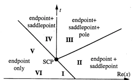
In figure3 wedisplaytheoverall combination of termsthatcontribute from the

sum

of the four

integrais. For theintegrals $I_{3}(x;\epsilon)$ andI4(x;$\epsilon$) a singleStokes line existsalongthe wholeof the

$t$-axis. Superposing thisonthe integrals $I_{1}(x,t;\epsilon)$ andI2(x,$t;\epsilon$)

we

find that the composite

ex-pansionhasa Stokes linealongthe$t$-axisfor$t>1/\sqrt{3}$, butnot for$t<1/\sqrt{3}$

.

This does not alter

the role of thehigher order Stokes phenomenon, which has determined the constituent Stokes

behaviour of$I_{1}(x, t;\epsilon)$ and$I_{2}(x, t;\epsilon)$. Hence, in regions$\mathrm{I}$, VIand$\mathrm{V}$ only the endpointsofthe

four integralscontributes to the asymptotics, InregionII and IV there

are

also contributions

Figure 3: The active and relevant Stokes lines together with the asymptotic contributions in

each region for thecomplete expansion of(2.1) generated bysumofintegrals in (2.2).

A furthersignificantconsequence of this example isthenecessity to includeexponentially sub

subdominant terms in the largetime asymptotic analysis. For $x>0,$$t\approx \mathrm{O}$, the dominance of

the asymptoticcontributions is (cf. (2.12),(2.13),(2.14))

$|e^{-f/\epsilon}eT^{(e)}|>|e^{-f/\epsilon}s_{1}T^{(s_{1})}|>|e^{-f/\epsilon}\mathrm{p}_{1}T^{(p_{1})}|$

.

(2.16)

The longer time behaviour inregion III involves all three such contributions, with $e^{-f_{B}/\epsilon}1T^{\{s_{1})}$

a decaying function of time but $e^{-f\mathrm{p}_{1}}/\epsilon T^{\langle p_{1})}$

independent of time. Consequently $e^{-f_{\mathrm{p}_{1}}/\epsilon}T^{(p_{1})}$

develops

as

the principletimeindependent oscillatory background to the montonic $e^{-f/\epsilon}eT^{(e)}$

.

If the sub-subdominant $e^{-h_{1}/\epsilon}T^{(\mathrm{p}_{1}\rangle}$

had been initially neglected as irrelevant near to $t=0$,

then anincorrect large $t$, finite-x behaviourwould have beenpredicted.

This

can

beverified by

carrying out

a

similar analysisfor the other integrals $I_{2},$ $I_{3}$,

I4

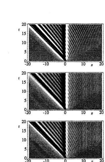
and combining the results.

In figure 4 we display a comparison ofa numerical evaluation ofthesum ofthe four integrals

in (2.2) in the real $($$,$t)$-plane against the leading order behaviours ofthe asymptotics _within

each Stokes regionfor the $\epsilon=$ 0.125. The plot in the middle of figure 4 is the

sum

of

the four

integrals, evaluatednumerically. The brightnessindicates the height. Theplot at the bottom of

figure4is the result of taking justtheleadingorder behaviours ofallasymptotic contributions

in each region as detailed in figure3.

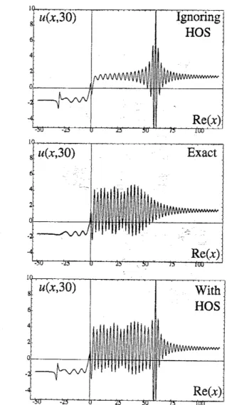
In figure 5 wetake

a

section for$t=30,$ $\epsilon=0.5$and plot the spatialdependence _of

solutions and

approxim ations. Theplotat the top is theleadingorderasymptotic approximationthat started at $t=0^{+}$ _{by ignoring the initially subsubdominant} $e^{-fp_{1}}/\epsilon T^{(p_{1})}$

.

The middleplot is the exact

solution. The bottomplot is the leading orderasymptotic _{evolved according to the activity} of

Stokes lines.

Figure 4: The plot in the middle is the solution of the PDE (2.1) minus $\arctan x$ with $\epsilon=$

0.125. The plot at the bottom is the resultof taking leadingorder behaviours of all asymptotic

contributions in each region (seefigure3), andthe plotat the top is the same, except that the

contributions from the sub-subdominant poles is omitted.

asym ptotics arising froma neglect of the sub-subdominant pole (top plots) ishowever at odds

with the exact result in region III. The exact

wave

structure is dominated at larger times

in this region by the initially sub subdominant pole contribution A neglect of this would have

resulted in

a

false conclusion being drawn

as

to the largetime behaviour. Finaliy only in the

neighbourhoods of the active Stokes

curves

do we observe that the sum of the leading order

behaviours changes discontinuously,

This example clearly demonstrates that the real time evolution of the solution of

even

linear

PDEsmay be affectedby the change in activity of Stokes

curves

caused byhigherorder Stokes

Figure 5: Theplot inthemiddle isthe exact solution of the PDE (2.1) at$t=30$ _{obtained from}

quadraturewith$\epsilon=0.5$

.

Theplot at thebottom_is

the result of taking leading orderbehaviours

of all asymptotic _{contributions in each region andthe plot at the top is thesame, except that}

the contributions from the

_{sub-subdominant}

_{poles is omitted. The disagreement between the}

exact and asymptotic approximations

near

to$t=-30$ and $t=60$isdue to the proximity of the

turning points TP in the complexplane at $x=2t+\mathrm{i}$ and $x=\mathrm{i}-t$ which

cause

the leading

orders to be the smallest term in the expansion,i.e., aman-uniformasymptoticanalysisbecomes

recent literature see for$\mathrm{n}$ example (but not exclusively), Costin

&

Costin (2001), Costin

&

Kohut (2004), Costin

&

Tanveer (2004), Olde Daalhuis $(2004\mathrm{a}\mathrm{b})$

.

We provideanoverview ofthe workhere, asthedetails willappearelsewhere Howls et$al$(2005).

Westart with the Burgers equation

$u_{t}+uu_{x}=\epsilon u_{xx}$, (3.1)

where

$x\in C$, $t\geq 0$, $\epsilonarrow 0^{+}$, (3.2)

and chooseinitial Cauchyconditions

$u(x, 0)= \frac{1}{1+x^{2}}$, and $uarrow \mathrm{O}$ as $|x|arrow\infty$. (3.3)

Obviously, Burgers equationmaybesolvedusing theCole-Hopfintegral representation,orusing

approximate matching techniquesto locate theposition of the smoothed shockthatform $\mathrm{s}$after

afinite time. Howeverwe shall approachthis pedagogicalexamplefroman exponential

asymp-totics pointof view toprovidean alternative, novel,view ofthe smoothed shock formation.

The small $\epsilon>0$ expansion of thesolution

can

be deduced tohave atemplate of the form

$u(x, t; \epsilon)\sim u^{(0)}(x, t;\epsilon)+\sum_{n=1}^{\infty}C_{1}^{n}u^{\langle n,1)}(x, t;\epsilon)+\sum_{n=1}^{\infty}C_{2}^{n}u^{(n,2)}(x, t;\epsilon)$ (3.4)

where

$u^{(0)}(x, t;\epsilon)$ $\sim$ $\sum a_{r}$$x\infty$( ,th)$\epsilon^{r}$ (3.5) $\tau=0$

$u^{(n,j)}(x,t;\epsilon)$ $e^{-nj_{j}(x,t)/\epsilon} \sum_{r=0}^{\infty}a_{r}^{(n_{I}}’)(x, t)\epsilon^{r}$, $j=1,2$, $n=1,2,3,$$\cdots$

.

(3.6)

By substitution into (3.1) we seethat $a\mathrm{o}(x, t)$ satisfies theinviscid Burgersequation

$\frac{\partial a_{0}}{\partial t}$

and for$r\geq 1$ the $a_{r}(x, t)$satisfy

$\frac{\partial a_{r}}{\partial t}+\sum_{\epsilon=0}^{r}a_{r-s}\frac{\partial a_{s}}{\partial x}=\frac{\partial^{2}a_{r-1}}{\partial x^{2}}$, $a_{r}(x_{r}0)=0$

.

(3.8)

The leading orders of the largest of the subdominantexponentialcontributionssatisfy$\emptyset(e^{-nf/\epsilon})$

generates

$\frac{\partial a_{0}^{(1\mathrm{j})}}{\partial t}+(a_{0}+2f_{x})\frac{\partial a_{0}^{(1,j)}}{\partial x}+(\frac{\partial a_{0}}{\partial x}-a_{1}f_{x}+f_{xx})a_{0}^{(1,j)}=0$,

(3.9)

Theexponentialfunctions $fj(x, t)$ _satisfythe first order nonlnear equation

$f_{t}+a_{0}f_{x}+f_{x}^{2}=0$. (3.10)

The boundary data for these functionscanbefound byconsiderationofthe rays of (3.7).

Therearethreeraysof (3.7) through each point $(x, t)$

.

These

are

the lines

$x=xj+a\mathrm{o}(xj)t$, $j=0,1,2$, (3.11)

where here and henceforth,

we

have abbreviated $a_{0}(x_{j}, 0)$ to $a_{0}(x_{j})$ and the $x_{\mathrm{J}}$

are

the

inter-section pointsofthese rays with the complex plane $t=0$, or_{alternatively, the locations of the}

saddlepoints in the Cole Hopf solution. On these raysthe$a_{0}$ take the constant values

$a_{0}(x_{\mathrm{J}})= \frac{1}{1+x_{j}^{2}’}$ $j=0,1,2$

.

(3.12)

Theroot $x\mathit{0}$of (3.11) is chosen to be the

one

that is real for all real $(x, t)$

.

The

families of rays

generated by the$x_{j}$ are tangential at caustics which simultaneouslysatisfy (3.11) and

$0=1+ \frac{da_{0}(x_{j})}{dx_{j}}t$, $j=0,1,2$, (3.13)

For thechosen initial conditions the causticsaregiven by

$t= \frac{2}{27}(x(x^{2}+9)\pm(x^{2}-3)^{3/2})$. _(3.14)

Since we restrict ourselves to$t>0$ _{the caustics}

_are

_{one-dimensional}

_curves.

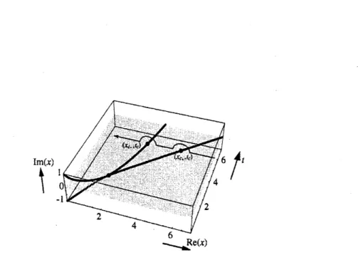
_{Thereare two real}

and twocomplex caustics in the $(x,t)$ space under consideration,

see

_{figure 6. Onthe complex}

caustic with $\Im x>0$_{, roots} $x_{0}$ and$x_{1}$ coalesce and

so we

call this caustic $c_{01}$

.

On thecomplex

caustics with $\Im x<0_{\}}x_{0}$ and$x_{2}$ coalesce and is thus labelled $C_{02}$

.

Onthe real caustics $c_{R},$ $x_{1}$

and$x_{2}$ coalesce.

These caustics$c_{R}$ separate the regions in the real _$(x,t)$

plane in which the classical smoothed

shock of Burgers’ equationforms (‘inside’ thecaustic) from regions where theamplitude

or

the

Figure 6: Caustics in complex $x$-space for real $t$ and

a

path of analytic continuation around

them.

Figure 7: Rays and caustics for Burgers’ equationwith initial data (3.3) for$x,$$t\geq 0$

.

The real

As$x_{1}$ and$x_{2}$ arecomplexoutside$C_{R}$, impositionof realityonthesolution is sufficienttoensure

uniqueness ofthe solution in the real $(x, t)$ planeoutside thereal caustics. The uniquesolution

to theinviscid Burgers’ equationoutside the caustic in the real $(x, t)$planeisthus $a_{0}(x_{0}(x, t))$

.

It isobvious, andwellknown, thatinside $C_{\mathcal{R}}$,the multivalued leadingorder invisicid behaviour

$ao(x, t)$ that satisfies the inviscid _Burgers’ equation cannot _adequatelyrepresent the_solutionof

viscid Burgers’ equation. By using exponentialasymptotics the effectofthemultivaluednessof

$a0(x, t)$ may becorrected.

Note thatthe$a_{0}$appearingin (3.10)isidentical to thechoiceof$a0$in the leading order behaviour

$u0$ in (3.5) . It istherefore $a_{0}(x_{0}(x, t))$, which iscompietely determined by (3.7), where$x_{0}(x$,?$)$

is the real solution of (3.11).

The exponents $f_{j}(x, t)$ must vanish on the complex caustics, since here they coalesce with the

exponentoftheleadingordersolution,i.e., $f_{0}(x, t)\equiv 0$,sothat the exponential correctionterms

arethere of thesame order

as

thefirstseries in (3.4). Thus theboundary data forthe solutions

of (3.10) are

$f_{j}(x, t)=0$ on $C_{0j}$, $j=1,2$

.

(3.15)

and

$f1(x, t)=f_{2}(x, t)$ on $C_{R}$. (3.16)

Cole-Hopf, ordirect analysis of thePDE reveals that

$f_{j}(x(x0, xj),$$t(x0,xj))= \frac{1}{2}\int_{x_{0}}^{x_{j}}a_{0}(z)dz-\frac{1}{4}(a_{0}(x_{0})+a_{0}(x_{j}))(x_{j}-x_{0})$, (3. 17)

$j=1,2$

.

It can also be shown that

$a_{0}^{(1,1)}(x_{0}, x_{1})=(a_{0}(x_{1})-a_{0}(x_{0}))\sqrt{\frac{a_{0}(x_{1})-a_{0}(x_{0})-a_{0}’(x_{0})(x_{1}-x_{0})}{a_{0}(x_{1})-a_{0}(x_{0})-a_{0}’(x_{1})(x_{1}-x_{0})}}$. (3.18)

This resultsholdsfor all values of$x0$ and$x_{1}$

.

We

now

turn tothe singularitystructureinthe Borelplane. It is actuallyalotmorecomplicated

than weshall outlinehere (seeHowls et

at

2005). However forthepurposes of this paper it will

suffice to consider thefollowing simplified story.

The location of singularities visible from $\tau=f_{0}(x, t)$ are indicated in figure 8 for

a

typical

value of$(x, t)$. Rom(3) wededuce _thatin the Borel_{plane, (logarithmic) branch-points exist at}

$\tau=nfj,$ $j=1,2,$ $n=1,2,3,$$\cdots.$ Adetailed analysis of thetransseries (see e.g., Olde Daalhuis

$2004\mathrm{a}\mathrm{b})$ or the Cole-Hopf

rePresentation

shows that the Borel transform of_{$u^{(1,1)}(x, t;\tau)$}

must

see a branch-point at $\tau=f_{2}(x, t)$

.

Likewise the Borel transform of $u^{(1,2)}(x, t;\tau)$ must see a

degenerate to a pair ofturning points. Due to symmetry of the initial conditions as $|x|arrow\infty$

we shall also initially just considerthe continuation around the turning point with the largest

values of$\Re x$. We label thispoint $x_{\mathrm{c}+}$

.

We take a path in the complex $x$-plane along the points $xA,$ $xB,$ $\cdots$, see figures 6, 8. This

complex path is taken to avoid any singular behaviour in the exponentially

sm

all transseries

$u^{(n,1)}$ and$u^{(n,2)}$, ($u^{(0)}$ is actually regular at _{$C_{R}$}), which neverthelesswillplay avital role inside

thecaustic region. It isobviously possible toobtainauniform asymptotic approximation

across

the caustic involving Airy functions. However we

are

interested here in the morefundamental

exponentialasymptoticbehaviour thatunderpins other procedures.

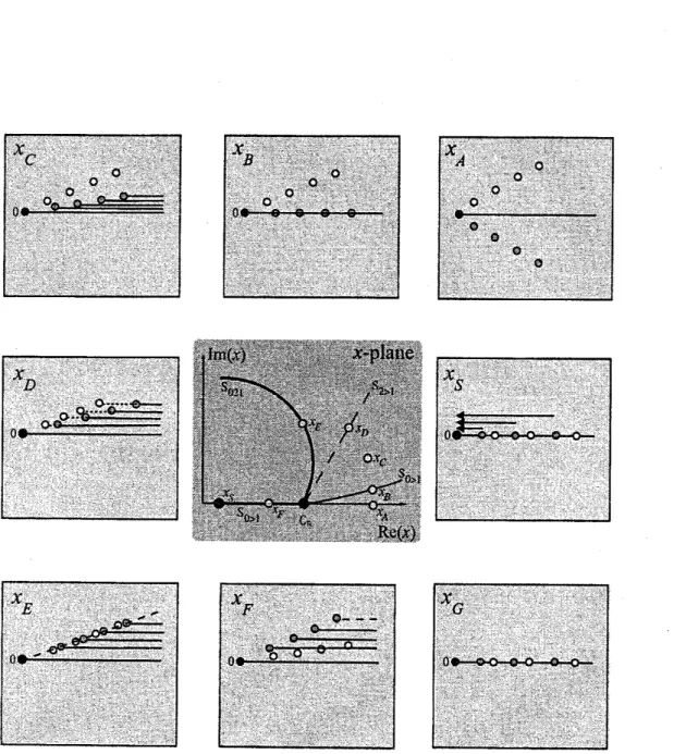
Surroundingthe centraldiagramof thecomplex$x$-planeinfigure8,aresnapshotsofthelocations

of the singularities as viewed from $\tau=f_{0}$ in the Borel plane at the positions $x_{A},$ $x_{B},$ $\cdots$

.

As

we move aroundthe complex$x$-plane, the arraysofsingularities willpivot about $fo=0$.

We alsoplot thesections throughthe Stokes surfaces $S_{i>j}$

across

which contributions involving

$f_{i}$ can switchon $f_{j}$

.

Note that at the turning point $x_{c+}f_{1}=f_{2}>0$, hence this turningpoint

does not directly involve$f_{0}$

.

Thus theStokes lines $S_{0>1}$ and$S_{0>2}$both passthroughtheturning

point inertly and$f_{0}$ dominates $f_{1}$ and $f_{2}$ all along thisline in the vicinity of$x_{c+}$. On the other

hand theStokeslines$S_{1>2}$ and$S_{2>1}$ sprout at angles of$2\pi/3$from $x_{c+}$ (reflectingthe Airy-type

nature of the simple coalsecence). A higherorder curve $S_{021}$ exists for $(x,t)$ in the locality of

$x_{\mathrm{C}+}$ and is also showninfigure8. Note thata branchcutalsoemanatesfrom$x>x_{c+}$. However,

1n what followswe

can

avoid all interaction withit, andso for simpiicity wehave not included

it in the figure.

It transpires Howls et al (2005) that we only actually have to consider the Stokes lines $S_{0>1}$, $S_{0>2},$ $S_{1>2}$ and $S_{2>1}$.

We now start on the real $x$-axls outside the caustic regionwhere $x>x_{\mathrm{c}+}$

.

Wepick a general

point$x_{A}$, and aim to continue to$x<x_{c+}$in thecomplex$x$-plane. At$x_{A}$,tosatisfythedecayof$u$

as$|x|arrow$ oo(3.3), comparison ofthe fulltemplatefortheexpansion (3) reveals that$C_{1}=C_{2}=0$

.

Hence

we

have

$u(x_{A},t\cdot, \epsilon)\sim u^{(0)}(xA,t;\epsilon)$, $(3,19)$

as thecomplete asymptotic expansion.

At $x_{B}$ we

cross

the Stokes line $S_{0>1}$. Here the array of singularities$nfi,$ $n=1,2,3,$

Figure 8: The central panel depicts part ofthecomplex$x$-plane at constant $t>8/\sqrt{27}$for

ex-pansion (3.4) andillustrates thelocation of Stokesand higher order Stokes

curves.

Surrounding the central panel

are

snapshots of the distribution of singularities in the Borel plane,

as seen

from $f_{0}$, at the various values of_$x$ indicated. See the main text for

a

fulldescription of what

a Stakes We canshow (either fiiom Cole-Hopfordirectlyfrom the PDE

that $K_{01}=1$

.

At $x_{D}$ weencounter the Stokes lne$S_{2>1}$. At thispoint singularity _{$f_{1}-f_{2}>0$}andsothereisa

potentialfor aStakesphenomenonto takeplace. However, singularity $f_{2}$ isnot contributingto

the transseriesexpansion of the functionwe

are

interested inat$x_{D}$. Hence

no

Stokesphenomenon

between$f_{2}$ and$f_{1}$ actually takesplace andthis is againanirrelevant Stokescurve,

At$xE$,weencounterthe higherorder Stokesline$S_{021}$. Onthiscurvethe Borelsingularities$f_{0},$ $f_{1}$

and$f_{2}$ and all theirmultiplesarecollinear. Herewe seethatratherthan havingafinite number

ofcollinear singularities, we must deal with and infinite set, leading to an infinite number of

Riemannsheets.

As inlinear cases, since $|fi|>|f_{2}|$, on theline ofcollinearity in the Borelplanethe singularity

$f_{2}$ lies in between

$f_{0}$

and $f_{1}$. Whenwe crossthehigher order Stokesline, when viewed from$f_{0_{i}}$

thesingularity at

$f_{1}$

moves across acut from $f_{2}$ andonto adifferent Riemann sheet from

$f_{0}$

.

A more detailed analysisofall the othersingularitiesHowls et $al$ (2005) showsthat oncrossing

thehigherorderStokesline allthe singularitiesinthearray$f_{1},2f_{1},3f_{1},$ $\cdots$ move ontomutually

different Riemann sheets and

are

so

are

directly invisible fromthe original expansion point $fo$,

and thesingutarities$nf_{1}$ can

no

longer see$mf_{1},$ $m\neq n$

.

At $xF$, the arraysare no-longer collinear with one another. However the $nf_{1}$

are

still collinear

with

$f_{0}$

: justbecause they might be on different Riemannsheets, this doesnot grant themthe

autono1nyto moveindependently.

At $x_{G}$, where $x$ is real, but _{$x<x_{c+},$}

$f_{0}$

and the arrays $nf_{i}$,$mf_{2}$

are

all again colinear, this

time along the horizontal direction of Borelintegrationand $0<f_{i}<f_{2}$. A Stokesline therefore

potentially exists between

$f_{0}$

and the $nf_{1}$. However, since the $nf_{1}$ are

now

all

on

different

Riemann sheetsfrom

$f_{0}$

, they

are

invisible to

$f_{0}$

and cannot cross the actual Borel integration

contour, which is anchored at

$f_{0}$

but on the principal Riemann sheets. Thus the the Stokes

line$S_{0>1}$ is inactive and no Stokesphenomenonbetween $f_{0}$ andanyelement of

$nf_{1}$

takes place.

There is also the possibility of a Stokes phenomenonbetween $f_{0}$ and $nf_{2}$ or

even

$fi$ and $nf_{2}$,

butthese are of lowerexponential order and will notconcern us here.

It isimportant

now

to recall that $\=x_{c+}$ isnot a turning point/caustic for0 and

$nf_{1}$

.

Hence

Stokes curve that passesthrough$\=x_{c+}$.

We mowexamine the structureof the‘dominant’ part ofthe transseries on the real$x$-axlsinside

$c_{R}$

$u(x, t; \epsilon)=a0(x, t)+\sum_{n=1}^{\infty}K_{01}^{n}e^{-nf1(x,t)/\epsilon}a_{0}^{(n,1\}}(x, t)+O(\epsilon)$ , (3.21)

as $\epsilonarrow 0+$

.

Exponentially small terms are included before the 0$(\epsilon)$ in (3.21) because we are

now in a region where $fi(x, t)$ may decrease to zero. _{There is thus} the possibility that these

exponentially small termscaninterferewith the $O(1)$ terms.

We combine (3.5), (3.6) and (3.10) and areable to deduce for $n=2,3,4,$$\cdots$, that

$a_{0}^{(n,1)}=(a_{0}^{(1,1)})^{n}(-2 \frac{\partial f_{1}}{\partial x})^{1-n}$ (3.22)

This simplerelationship allowsus to sum then-sum in thetransseries (3.21) and obtain

$u(x, t;\epsilon)=a0_{\backslash }^{(_{X}},$$t)+ \frac{2K_{01}a_{0}^{(1,1)}(x,t)^{\partial}\neq_{x}^{1}e^{-f_{1}/\epsilon}}{2\frac{\partial f_{1}}{\partial x}+K_{01}a_{0}^{(1,1)}(x,t)e^{-f\iota/\epsilon}}+O(\epsilon)$, (3.23)

as $\epsilonarrow \mathrm{O}+$. Thisresult isvalideverywhere in theregion where

$\Re f_{1}>0$and may beanalytically

continuedto the region where$\Re f_{1}\leq 0$.

If we continue along the iine $S_{0>1}$, in the negative $x$-direction the singularities $nf_{1}$ all move

towards $f_{0}$ in the Borel plane, see_{$x_{H}$}. At the point _{$(x_{S}, t)$} the $nf_{1}$ appear to coalesce with $f_{0}$

.

This is the point at whichan exchange of dominance in the asymptoticexpansion stakes piace.

Classically,thisistheposition of thesmoothed shock, where the solutionchangesabruptly ffom

one valueto thenext.

Due to the coalescence of the exponents, from a naive point ofview, this point is apparently

a caustic/turning point of the asymptotics. Ifthis were a true turning point the derivatives

in individual terms in theasym ptotics would diverge at $x_{S}$

.

An examinationofthe coefficients

$a_{r}(x, t)$(Howls et$al$2005)shows that this is not thecase. The

reason

_{for this}

is that,

as

suggested

above,atl thesingularities$nf_{1}$ and0 indeed do lie on mutttally

different

Riemann sheets: this is

only an apparentcoalescence. This is avirtualturning point.

We may now conclude with thefollowing keyobservations (further discussionmay be found in

Howls $al$2005).

The terms themselves in the transseries do not diverge at theposition of the smoothed shock

$xs$. This is because $xs$ is only

a

virtualturning point, since all the Borel singularities are on

mutualiy different Riemannsheets, _{Hence the Borel singularities have accumulated to createa}

Hence, when viewed from the standpoint of exponential asym ptotics, the higher order Stokes

phenomenon is an essential part of the mechanism for forming the smoothed (propagating)

shock.

The resummed transeries solution (3.23) is valid for values of$\<xs$

.

It is thus a way of

con-tinuingthesolutionthrough thenonlinearanti-Stokes linethatpasseslocally vertically through the virtual turning point.

Althoughthis isonlyonespecificsmoothed shockproblem,we believe the mechanismexplained

above ismoregeneral. Clearly asmoothed shockisachange of dominancebetweencontributions

in an expansion. If these take the formof exponentially prefactored series, then a Borel plane

structuresimilarto that described above will exist. If theboundarydata issuch that (infinitely)

many singularities arecontributing to the asymptotics near to the smoothed shock, andif the

asym ptotics does not diverge at that shock, then the Borel singularities must lie on mutually

different sheets. This may well have arisen because of the crossing of a higher order Stokes

curve.

4

Conclusion

In this paper we have concluded the discussion of the higher order Stokes phenomenon by

showingits relevanceto thelarge timeasymptotics oflinearPDEproblemsand smoothedshock

formation ina nonlinearPDE.

The relevance ofthe higher order Stokesphenomenonto aproblem will be determined bothby

the problem andthe boundary dataassociated with it. The difficultyin practicallyexam ining

its effects inODEsor PDEsshouldnot be underestimated. Nevertheless in canonicalproblems,

some progress

can

be made and extra insight

can

be obtained into the underlying analytic

Acknowledgements

This work vas supported by EPSRC grant GR/R18642/01 and by a travel grant from the

ResearchInstitutefor MathematialSciences, UniversityofKyoto.

References

Costin, O. , Costin R.D., 2001, On the

formation of

singularities

_of

solutions

_of

nonlinear

differential

systems in antistokes directions, Inventiones Mathematicae 145, 3, pp425-485.

Costin, O. , Costin R. D., Kohut M., 2004, Rigorous bounds

_of

Stokes constants

_for

some

nonlinear ODEs at rank one irregular singularitiesProc. Roy. Soc. Lond.. In Press

Costin, O, Tanveer, S. ,2004, Nonlinear

_evolutionof

PDEs in$\Re^{+}\cross C^{d}$ : existence anduniqueness

of

solutions, asymptotic and Borel summability, preprint Rutgers University.

Howls, C. J., LangmanP., OldeDaalhuisA. B. , 2004, On thehigherorder Stokesphenomenon

Proc. R. Soc. Lond. A 460, 2585-2303.

Howls, C.J. ,2005a, When is a Stokes line not

a

Stokes line? I. The higher order Stokes

phe-nomenon, this volume.

Howls, C.J. , 2005b, When is a Stokesline not aStokesline? II. Examples involving

_differential

equations, thisvolume.

HowlsC.J., OldeDaalhuis A.B., 2005, When is ashock not a caustic9 _{In preparation.}

Olde Daalhuis, A. B., 2004a, Hyperasymptotics for nonlinear ODEs I: A Riccati equation,

submitted to R. Soc. Land. Proc. Ser. A Math. Phys. Eng. Sci.

OJdeDaalhuis, A. B., 2004b, Hyperasymptotics for nonlinear ODEs II$.\cdot$ The firstPainleve’

equa-tion andasecond orderRicattiequation, submittedto R. Soc. Lond. Proc. Ser. AMath. Phys.