Regional Differences of the Driving Factors and Decoupling Effect of Carbon Emissions : Evidence from China's Pollution-Intensive Industry

and Decoupling Effect of Carbon Emissions : Evidence from China's Pollution‑Intensive Industry

著者 Lafang Wang, Xia Liu, Meimei Tan journal or

publication title

International Review for Spatial Planning and Sustainable Development

volume 4

number 4

page range 4‑26

year 2016‑10‑15

URL http://hdl.handle.net/2297/46679

doi: 10.14246/irspsd.4.4_4

4

DOI: http://dx.doi.org/10.14246/irspsd.4.4_4

Copyright@SPSD Press from 2010, SPSD Press, Kanazawa

Regional Differences of the Driving Factors and Decoupling Effect of Carbon Emissions

Evidence from China's Pollution-Intensive Industry

Lafang Wang

, Xia Liu

and Meimei Tan

1 School of Economics and Trade, Hunan University

* Corresponding Author, Email: [email protected] Received: May 01, 2016; Accepted: June 15, 2016

Key words: Pollution-intensive industry, CO2 emissions, Completed decomposition technique, Decoupling analysis, Reduction potential

Abstract: The completed decomposition model combined with the decoupling index is used to analyze the contribution of each factor which influences energy- related CO2 emission in 15 regions over the period 2000-2012. The results show that the major factors that influence CO2 emission in areas are industrial output effect and energy intensity effect, followed by the industrial structure effect, while the energy structure and energy emission intensity have a smaller effect. Moreover, a reduction potential model is implemented in order to investigate the emission reduction potential of regions and sub-industrial sectors. It is found that although most governments showed great enthusiasm in promoting emission reduction, most regions present no decoupling effect. It indicates that emission reduction efforts have not always proven effective till now, therefore, most regions, including Beijing, have great energy saving and emission reduction potential.

1. INTRODUCTION

The Chinese Government has promised a CO

intensity target of 40%- 45% reduction by year 2020 compared to 2005 levels, but the situation of its carbon emission ranking first in the world makes this task difficult to fulfil.

How to implement the emission reduction policies at the industry level is key to realize this target. At present, China's economic growth is still in the pattern of growth led by manufacturing. So, although China has taken important measures to reduce its carbon emission, a sustainable high growth rate of manufacturing, especially of pollution-intensive ones, is still the main driving force of the rapid growth in CO

emissions.

Chinese natural resources are unevenly distributed and there have been

big economic development differences in regions, which lead to an obvious

regional difference in carbon emissions (Liu, Z. et al., 2010; Xiong et al.,

2012). Many studies have focused on China’s energy-related CO

emissions

and some important opinions have been gained from the existing literature

regarding the driving factors of CO

emissions (Wang, C., Chen, & Zou,

2005; Xu, Xu, & Hu, 2011). Unfortunately, there are very few studies with

respect to the driving factors of CO

emission from a regional perspective

(Li, Song, & Liu, 2014; Wei, Ni, & Du, 2012; Yi et al., 2011). Hardly any

comparison of CO

emissions at the regional level from the perspective of

pollution-intensive industries has been done. Therefore, it is necessary to investigate the driving forces of CO

emissions in the pollution-intensive industries and realize a deeper understanding of how CO

emissions related to pollution-intensive industries have evolved in regions. To achieve this goal, the proper approach needs to decompose the CO

emissions into the possible factors that affect such emissions. In this way, we can get a deeper understanding of the strengths and weaknesses of each region regarding their emission performance.

There are a variety of methods that can be used to decompose the CO

emissions, such as Structural decomposition analysis (SDA), IPAT equation, Divisia index decomposition analysis (Divisia IDA), and Laspeyres index decomposition analysis (Laspeyres IDA). The SDA method has been used in many studies (Tukker & Dietzenbacher, 2013; Wiedmann, 2009). However, it is based on an environmentally extended input-output table which is published every five years. Although the interval of data for four years can be calculated, it is built on a series of assumptions, the reliability is not high, and the economic development situation changes very fast. Therefore, SDA cannot fit the needs of research. For the IPAT equation, it is mainly used to analyze the impact of human activities on the environment, which reflects the influence of population, output and technology on CO

emissions (Dietz

& Rosa, 1994; Ehrlich & Holdren, 1971). The IPAT equation does not take other factors such as the energy use into account. Divisia IDA and Laspeyres IDA use the index concept in decomposition (Hoekstra & Van den Bergh, 2003), which has been used in many studies on CO

emissions’

decomposition due to the abundant availability of data. Although it has been proved by Ang (2004) and Greening et al. (1997) that there is a stronger theoretical basis in Divisia IDA than that in Laspeyres IDA, because there is a large residual term after decomposition in the traditional Laspeyres IDA, the Laspeyres IDA does have some advantages compared with others (Diakoulaki & Mandaraka, 2007; Xu, Xu, & Hu, 2011). Sun (1998) improved the Laspeyres IDA, modifying it into a complete decomposition technique, which eliminates the un-decomposed residual term, and makes the results more accurate. According to these advantages and disadvantages of above decomposition methods, this research employs the complete decomposition technique to decompose the CO

emissions.

The decomposition of carbon emissions can reflect the impact of each factor on carbon emissions, and tell us which factors determine the change of CO

emissions in different regions of China’s pollution-intensive industries over the examined time. However, the degree of decomposition analysis is not sufficient for full examination of changes that took place in each area and sub-sector separately, and cannot show: (1) what reduction efforts have been done contributing to the maximum decline of the CO

emissions in each region? (2) Is there a regional difference in the relationship between development and emission reduction? (3) What is the reduction potential of CO

emissions of the pollution-intensive industries and how high can this be?

To answer the question (1) and (2), the proper approach is to try to determine the decoupling process of industrial growth from the CO

emissions level and to realize the joint exploitation of the factors identified

in the complete decomposition analysis. This decoupling was proposed by

OECD in 2002 firstly (Organization for Economic Co-operation and

Development, 2002). As an important concept for integrating economy and

environment (Enevoldsen, Ryelund, & Andersen, 2007; Wang, W. et al.,

2013), it breaks the relationship between environmental damage and

economic wealth, or the relationship between environmental pressure and economic performance. The decoupling theory has been widely used in many studies. The main methods adopted were the comprehensive analysis of variation method, the decoupling index method, the elastic analysis, the decoupling analysis method which is based on a complete decomposition technique, the statistical analysis method, the econometric analysis method and the differential regression coefficient method (Zhong et al., 2010).

Among them, the decoupling index method is more widely applied. The decoupling index method and the elastic analysis are mainly focused on studying the relationship between economic growth and CO

emissions and they do not take other influence factors into account; the econometric analysis method and the differential regression coefficient method have high demand in data. Considering the availability of data and the purpose of this paper, we will choose the decoupling analysis method which is based on complete decomposition technique as a tool.

The third question implies an assessment of the gap between the optimal value and the real value of emission reduction. Although sample areas are regions of China, they show big differences in their levels of industrial development and industrial structure. Moreover, other obvious distinctions such as the availability of natural resources and the historical attachment to particular industrial activities make assessment a rather important task.

The remainder of this paper is organized as follows: Section 2 introduces the definition of pollution-intensive industries. Section 3 presents the methodology and the data. Section 4 provides the result and discussion.

Section 5 contains concluding remarks.

2. DEFINITION OF POLLUTON-INTENSIVE INDUSTRY

According to the existing literature, pollution-intensive industries are generally considered to be those who produce large amounts of pollutants in the process of production or sales, but there is no consistent definition in current academia for this kind of industry, and also no uniform standard to define it. The current way of definition can be roughly divided into the following categories:

a) Calculating the index of pollution emission uses multiple indicators, such as industrial wastewater, waste gas and solid waste. And then the industry can be divided into high, middle, low pollution industries and cleaning industry (Liu, Q., Wang, & Li, 2012). The advantage of this method is that it can distinguish whether the industry is polluting industry or not, but it cannot distinguish the industry pollution types.

b) Judging by the degree or scale of pollution or contamination uses a single indicator, such as emissions scale or emissions intensity.

Generally, the emissions scale is the sum of different kinds of pollutants.

However, this method does not take the different properties of each pollutant into account.

From what has been mentioned above, in this paper, we take those two aspects into account when we define the pollution-intensive industries.

Step 1: Classify the type of pollutant. To achieve this, two indicators,

including the emission intensity and emission scale, are constructed. Their

calculation formula can be expressed as follows:

i ij

ij X

EI XE

(1)

ET

ES_ij XE^ij

(2)

where EI

and ES

denote the emission intensity and the emission scale of j pollutant in industry i; XE

denotes the j

pollutant emission quantities of the i

industry; X

is the industrial production of the i

industry;

while ET is the total industrial added value. Using the relevant data of 2010, EI

and ES

can be calculated.

Step 2: Calculate the pollutant index of each type. The pollutants are divided into three categories: water pollutant which is measured by wastewater emissions, gas pollutant which is measured by the emission of SO

, dust and smoke dust, and solid waste which is measured by solid waste emissions. Based on Equation (1) and Equation (2), the normalization process is shown as follows:

) min(

) max(

) min(

ij ij

ij ij

ij EI EI

EI EI EI



 

(3)

) min(

) max(

) min(

ij ij

ij ij

ij ES ES

ES ES ES



 

(4)

Based on Equation (3) and (4), the pollution index I

(where j is waste air, waste water and solid waste, respectively) of industry i can be calculated as illustrated in Equation (5):

12

( * )

ij ij ij

I  EI ES

(5) Table 1, below, summarizes the results of these three kinds of pollution indexes. Correspondingly, the pollution-intensity industry is sorted into three groups including high-water-pollution industry, high-gas-pollution industry and high-solid-waste pollution industry.

The scope of this paper is to analyse the decoupling process of industrial growth from the CO

emissions level in the pollution-intensive industries. As the high carbon emissions industry generally belongs to the high-gas- pollution industry, we chose the pollution-intensive industry according only to the result of high-gas-pollution industries. As shown in Table 1, there are seven typical high-gas-pollution industries, including electricity, heat production and supply, non-metallic mineral products industry, ferrous metal smelting and rolling industry, chemical materials and chemical products manufacturing, paper and paper products industry, non-ferrous metal smelting and rolling industry, and petroleum processing and coking and nuclear fuel processing.

All the data of high-pollution industries that Section 3 requires are calculated from these seven industries.

Table 1. The categories of pollution-intensive industry

Industry Waste air Waste water Solid waste Production and Supply of Electric Power and

Heat Power

1.0000 0.1602 0.4144

Manufacture of Non-metallic Mineral Products 0.5195 0.0400 0.0445 Manufacture and Processing of Ferrous Metals 0.2622 0.1254 0.2587 Manufacture of Chemical Raw Material and

Chemical Products

0.1349 0.3598 0.1015 Manufacture of Paper and Paper Products 0.1270 1.0000 0.0351 Manufacture and Processing of Non-ferrous

Metals

0.1151 0.0418 0.0811 Processing of Petroleum, Coking, Processing of

Nucleus Fuel

0.1129 0.1002 0.0317

Mining and Washing of Coal 0.0521 0.1779 0.2848

Manufacture of Textile 0.0396 0.3725 0.0067

Mining of Non-ferrous Metal Ores 0.0391 0.1612 0.7383

Manufacture of Beverage 0.0350 0.2018 0.0149

Manufacture of Chemical Fibre 0.0348 0.1536 0.0100

Mining and Processing of Non-metal Ores 0.0308 0.0331 0.0495

Manufacture of Foods 0.0297 0.1291 0.0096

Mining of Ferrous Metal Ores 0.0292 0.0482 0.6402

Processing of Food from Agricultural Products 0.0284 0.1926 0.0174 Processing of Timbers, Manufacture of Wood,

Rattan, Palm and Straw Products

0.0211 0.0114 0.0037

Manufacture of Medicines 0.0206 0.1222 0.0057

Manufacture of Rubber 0.0132 0.0204 0.0027

Manufacture of General Purpose Machinery 0.0116 0.0094 0.0045

Mining of Other Ores N.E.C 0.0113 0.0000 0.0195

Production and Distribution of Gas 0.0112 0.0075 0.0022 Extraction of Petroleum and Natural Gas 0.0086 0.0261 0.0031 Manufacture of Special Purpose Machinery 0.0082 0.0107 0.0021

Manufacture of Metal Products 0.0075 0.0498 0.0038

Manufacture of Transport Equipment 0.0067 0.0189 0.0034

Manufacture of Plastic 0.0059 0.0053 0.0008

Manufacture of Leather, Fur, Feather and its Products

0.0043 0.0789 0.0012

Manufacture of Tobacco 0.0032 0.0054 0.0007

Manufacture of Textile Wearing Apparel, Footwear and Caps

0.0028 0.0237 0.0006 Manufacture of Artwork, Other Manufacture

N.E.C

0.0026 0.0052 0.0006 Recycling and Disposal of Waste 0.0017 0.0034 0.0020 Manufacture of Electrical Machinery and

Equipment

0.0013 0.0000 0.0003 Printing, Reproduction of Recording Media 0.0010 0.0038 0.0002

Manufacture of Furniture 0.0010 0.0051 0.0003

Production and Distribution of Water 0.0007 0.2383 0.0009 Manufacture of Measuring Instrument and

Machinery for Cultural Activity and Office Work

0.0001 0.0126 0.0005

Manufacture of Communication, Computer and Other Electronic Equipment

0.0000 0.0305 0.0008 Manufacture of Articles for Culture, Education

and Sport Activity

0.0000 0.0018 0.0000

3. METHODOLOGY

3.1 Complete decomposition technique

The residuals decomposition method of the complete decomposition technique is based on the principle of “jointly created and equally distributed” (Sun, 1998). For example, the target variable Z can be decomposed as Equation (6):



 ⁿ i

x

1

(6) where X

denotes the i

factor of target variable Z, n denotes the number of factors. Z

and Z

denote the target variable in year t and in base year, therefore, Z

and Z

is the sum of X

(i.e. X

 X

  X

) and X

, respectively. Then the change in target variable recorded in time t in comparison with their level in a base year t=0 can be expressed as follows:

0 0 0 0

1 1 1 1

( )

n n n n

t it i i i i

i i i i

Z

Z Z x x x x x

   

   







 (7)

In this paper, n=5, thus  Z can be shown as Equation (8):

5 5 5 5

0 0 0 0

1 1 1 1

( )

t it i i i i

i i i i

Z

Z Z x x x x x

   

   







 ⁽⁸⁾

From Equation (8), we can see that  Z can be divided into two parts.

The first part is the first item, which reflects the change of  Z resulting from the individual factor change. This is also the only part of the traditional LMDI model. The second part is the rest and reflects the change caused by multiple factors.

According to the principle of the complete decomposition technique, the value in the second part should be assigned to each of the corresponding factors (Sun, 1998), and then we can obtain the contribution of each factor to the target variable, which is shown as Equation (9):

(9) In this paper, the target variable Z is CO

emission C

, thus, C

can be decomposed as follows:

x x x x x x

x x x x

Z

x x x x x

x x x

Z

x x x x

x x

Z

x x x

x x Z

x Z

r m k j i r

m k j

i i j k m r

m k j i m

k j

i i j k m

k j i k

j

i i j k

j i j

i i j

i

i i

effect

X



















 





 















 



 











 

 







 











































0 0 0 0 0

0 0 0 0 0

0 0 0 0

0

0 0

0 5

1 0

0

5 1 4 1 3 1

2

1

5 7 5 7 5

1 1 1 1 1

ikt jkt jkt

kt ikt kt ikt ikt jkt

kt jkt jkt

j i kt ikt j kt jkt i j

P

P E E C

C



C



P

P



E

E





(10)

where C

denotes the total CO

emission of k region in year t. It also can be expressed as the total CO

emission of k region resulting from the consumption of five types of energy. C

is the total CO

emission of the j

energy of k region in year t.

PS

reflects the output shares of sector i in k region (i.e. P

) within the total industry output of k region (i.e. P

) in year t.

EI

reflects the change in the ratio of energy consumption of sector i in k region (i.e. E

) to the total produced value of sector i in k region (i.e. P

).

ES

reflects the change in the share of energy forms in the total energy consumption of the pollution-intensive industry in k region. EF

is the CO

emission of industrial energy use in k region.

The change in CO

emission  C

during the period of [0, t] can be shown in Equation (11):

(11) Combing Equation (9), the changes in CO

emission  C

during the period of [0, t] can be decomposed into five parts as shown in Equation (12):

 C

 P

 P S

 E I

 E S

 E F

( 1 2 )

where P

is the industrial output effect, reflecting CO

emission changes of k region resulting from output changes in pollution-intensive industries;

eff

PS

is the industrial structural effect, reflecting CO

emission changes of k region resulting from structural changes in pollution-intensive industries;

eff

EI

is energy intensity effect, reflecting CO

emission changes of k region resulting from energy intensity; ES

is energy structural effect, reflecting CO

emission changes of k region resulting from the changes of the energy structure in pollution-intensive industries; EF

is energy source emission intensity effect, reflecting CO

emission changes of k region resulting from the changes of energy emission intensity in pollution-intensive industries.

The value of  C

in equation (12) is an absolute value (kt CO

). In order to better reflect the change in carbon emissions, the absolute value can be converted into the relative value (%) which is shown as a percentage:

0 e f f

k t k t

kt

k

M dC

dM C

  (13)

Here

0 kt kt

k

dC C C

  , M

 P

, PS

, EI

, ES

, EF

, respectively.

3.2 Decoupling analysis method

In reference to the definition given by Diakoulaki and Mandaraka (2007), the emission reduction is actually the result of all actions inducing a decline in the CO

emission of industrial production, such as optimizing the industrial structure, improving energy efficiency, and increasing the usage

F ES EI

PS P EF ES EI

PS P

C C C

jk j

jk ik

ik i

k jkt j

jkt ikt

ikt i

kt k kt kt

0 0 0

0 0 0

∑

∑

∑

∑

-























ratio of clean energy. These efforts correspond to the industrial structural effect PS

, energy intensity effect EI

, energy structure effect ES

and energy source emission intensity effect EF

. Therefore, for the government of region k, all the effort they made in year t (  F

) can be expressed as the sum of these four effect factors, that is:

 F

 PS

 EI

 ES

 EF

(14) Generally, when talking about low-carbon economies, this refers to an economy which is in the decoupling process between economic growth and greenhouse gas emissions, that is, the growth speed of the economy is faster than that of the CO

emission intensity (Guo, 2010). According to the decoupling theory, the decoupling index is measured by the ratio of environmental pressures to economic driving forces such as economic activities (Diakoulaki & Mandaraka, 2007). The value of  F

may take a negative sign if the sum of these four factors resulting in emission reduction.

Therefore, the decoupling index ( D

) can be expressed as Equation (15):

/ , 0

( ) / , 0

eff eff

kt kt kt

kt eff eff eff

kt kt kt kt

PS EI ES EF

F P P

D F P P P

D D D D

 

     

   

(15)

where D

indicates the industrial-structure decoupling index, D

indicates the energy-intensity decoupling index, D

is the energy- structure decoupling index, and D

reflects the energy-emissions-intensity decoupling index.

According to the above analysis, there are three values in this decoupling index D

:

a) If D

≤ 0 , it reflects no decoupling efforts. That is to say, emission reduction policies miss the mark or the policies have no effect. So the CO

emission still increases fast alongside the development of the economy.

b) If

D

, it means there is a weak decoupling efforts. This case suggests that the emission reduction policies have a certain effect, CO

emission is now slowing, but the reduction volume is less than the increase of emission caused by the development of the economy.

Therefore, the total CO

emission is still increasing.

c) If D

≥ 1 , it means there are strong decoupling efforts. It reflects that the emission reduction policies have an obvious effect in the reduction of CO

emission and lead to a larger volume reduction of CO

emission than the new growth resulting from the development of the economy.

3.3 Reduction potential

The above reflects the government’s carbon emissions reduction efforts, but it cannot reflect the reduction potential of the CO

emissions of pollution-intensive industries.

The reduction potential is the likelihood that emissions can be reduced.

Emission reduction potential of each region can be represented as follows:

(1

) *100

k

k

I CE

  CE (16) where

reflects the minimum of the carbon emission intensity among

all samples;

is the carbon emission intensity of the region k. Equation (16) implies that the carbon intensity of all areas will be close to the minimum value. The emission reduction potential of the lowest carbon emissions intensity of the region is zero, and the rest of the region varies from 0 to 100. The bigger the I, the bigger the emission reduction potential.

3.4 Data description

In this paper, the data comes from various issues of the statistical yearbook of provinces and cities. The industrial output was calculated at constant 2000 prices. Carbon emissions are the total emission of five energies used by seven high-pollution industries. Because the original data of energy consumption is in physical quantities, we convert the physical quantities to standard statistics firstly, and then use the standard coal consumption coefficient to calculate the total emission of each type of energy (Table 2). This method is more reasonable and accurate compared with the emission of end-use energy consumption. It needs every kind of energy consumption data of the seven pollution-intensive industries in regions, but the data in the statistical yearbook of some provinces is not complete. Therefore, this paper picks up fifteen typical provinces and cities as the subjects of study, including Beijing, Tianjin, Shanxi, Inner Mongolia, Liaoning, Jilin, Anhui, Fujian, Jiangxi, Henan, Hubei, Chongqing, Gansu, Ningxia and Xinjiang. The energy is composed of coal, coke, gasoline, diesel and electricity.

Table 2. The standard coal coefficient and carbon emissions coefficient of four energies Energy Standard

coal coefficient

(kgce/kg)

Carbon emission coefficient (tCO2/toe)

Energy Standard coal Coefficient

(kgce/kg)

Carbon emission coefficient (tCO2/toe)

Raw coal 0.7143 2.769 Gasoline 1.4714 2.029

Coke 0.971 3.314 Diesel 1.4571 2.168

The standard coal coefficient is referenced from "General principles for calculation of total production energy consumption" (GB/T2589-2008), and the carbon emission coefficient of energy, except electricity, is calculated in reference to the IPCC Carbon Emission Calculation Formula (2006 edition).

The carbon emissions coefficient of electricity is not fixed because the power generation technology in cities and provinces is different. Therefore, we calculate the carbon emissions coefficient of electricity in reference to the method of Fu (2011). The standard coal coefficient and carbon emission coefficient of five energies are shown in Table 2 and Table 3.

Table 3. Carbon emission coefficient of electricity in ten provinces and cities: 2000-2012 (tCO2/toe)

BJ TJ LN JL FJ SX NMG HN

2000 7.04 7.54 7.85 6.67 3.97 8.3 8.06 8.33

2001 7.03 7.39 7.7 6.35 3.65 8.14 8.03 8.09

2002 7.00 7.39 7.72 6.79 4.42 8.11 7.99 7.99

2003 6.87 7.37 7.6 7.18 5.16 8.08 7.83 8.01

2004 7.01 7.28 7.49 6.87 5.76 7.98 7.47 8.71

2005 6.9 7.23 7.4 6.56 4.61 7.91 7.08 7.72

2006 6.66 7.19 7.42 6.99 4.55 7.63 7.51 7.44

2007 6.49 7.12 7.18 6.74 4.91 7.48 7.38 7.16

2008 6.21 7.16 6.98 6.4 4.78 7.14 7.24 6.89

2009 5.96 7.05 6.92 6.02 5.11 7.21 6.97 6.75

2010 5.79 6.83 6.5 5.52 4.43 7.02 6.63 6.66

2011 5.77 6.82 6.52 5.85 5.43 7.02 6.6 6.65

2012 5.35 6.75 6.17 5.59 4.5 6.85 6.43 6.37

HB AH JX CQ GS NX XJ

2000 4.07 7.71 6.35 6.77 4.72 7.45 8.28

2001 4.44 7.62 6.26 6.91 5.04 7.57 7.73

2002 4.54 7.48 6.1 6.54 5.44 7.56 7.64

2003 4.13 7.93 6.98 6.42 5.93 7.34 7.91

2004 2.97 7.53 7.04 6.27 5.48 7.27 8.00

2005 2.85 7.44 6.8 6.31 5.03 7.3 8.27

2006 3.29 7.41 6.28 6.67 5.17 7.26 8.12

2007 2.87 7.2 6.49 5.99 5.07 7.16 7.63

2008 2.3 6.98 6.11 5.4 4.93 6.98 7.53

2009 2.51 6.8 6.16 5.42 4.5 6.84 7.34

2010 2.68 6.72 5.93 5.31 4.81 6.7 6.81

2011 3.11 6.77 6.32 5.52 4.76 6.8 6.96

2012 2.62 6.56 5.44 2.44 4.73 6.52 6.47

Data resource: China Electric Power Yearbook from 2001 to 2012

Abbreviation note: BJ: Beijing City, TJ: Tianjin City, SX: Shanxi Province, NMG: Inner Mongolia Autonomous Region, LN: Liaoning Province, JL: Jilin Province, AH: Anhui Province, FJ: Fujian Province, JX: Jiangxi Province, HN: Henan Province, HB: Hubei Province, QC: Chongqing City, GS: Gansu Province, NX: The Ningxia Hui Autonomous Region, and XJ: Xinjiang Uygur Autonomous Region.

The other data used in this paper are presented in Table 4-Table 6, below.

Specifically, Table 4 shows total energy consumption in high-pollution industries and the consumption ratio of five energies. It can be seen that during the period 2000-2012, coal, accounting for 76% of total energy consumption, is the principal energy in all regions. The total energy consumption in each region is rising, and the average growth rate is 310%.

Among them, the highest growth rate of energy consumption is Xinjiang (729%), while the smallest one is Beijing (35%).

Table 4. Total energy consumption in high-pollution industries and the five energy consumption ratios for the years 2000-2012

Regions Year Raw coal Coke Gasoline Diesel Electricity Total (10^7ktoe)

BJ 2000 36% 46% 1% 1% 16% 929

2012 83% 0% 0% 1% 15% 1258

TJ 2000 48% 30% 1% 2% 19% 429

2012 32% 46% 0% 1% 21% 1815

SX 2000 85% 11% 0% 0% 4% 8224

2012 82% 12% 0% 0% 6% 22567

NMG 2000 86% 7% 0% 1% 6% 3165

2012 86% 6% 0% 0% 8% 23295

LN 2000 79% 13% 0% 0% 7% 6223

2012 69% 21% 0% 1% 9% 14573

JL 2000 84% 7% 0% 0% 8% 2141

2012 83% 10% 0% 0% 7% 6192

AH 2000 82% 11% 0% 0% 6% 2069

2012 82% 10% 0% 0% 8% 9461

FJ 2000 82% 6% 0% 2% 10% 1338

2012 77% 9% 0% 1% 13% 5879

JX 2000 71% 16% 0% 1% 13% 1268

2012 69% 20% 0% 0% 11% 4281

HN 2000 85% 7% 0% 0% 8% 5166

2012 89% 0% 0% 0% 11% 16483

HB 2000 83% 0% 0% 1% 16% 2048

2012 83% 0% 0% 0% 17% 5936

CQ 2000 75% 14% 0% 0% 10% 955

2012 71% 11% 0% 1% 17% 2503

GS 2000 73% 12% 0% 0% 14% 1426

2012 72% 12% 0% 0% 16% 5401

NX 2000 80% 5% 0% 0% 15% 719

2012 84% 2% 0% 0% 14% 5317

XJ 2000 87% 5% 1% 1% 6% 1103

2012 79% 10% 0% 0% 11% 9148

Table 5 denotes total output in high-pollution industries and the share of sub-sectors. The growth rate of output in high-pollution industries presents significant differences in both their reference values in 2000, as well as in their development with time. The maximum growth rate is Shanxi with a rate of 2300%, while the minimum one is Beijing with a rate of 214%. For most regions, Chemical, ferrous metals and electric and heat power are the main sectors which account for more than 50% in output, but the new increasing areas of the economy in some regions have transformed chemical to non-metals and non-ferrous metals during the period 2000-2012.

Table 6 presents the energy intensities of the high-pollution industries and of seven sub-sectors calculated based on the data of Table 4 and Table 5.

With the exception of Xinjiang and Ningxia having increased energy intensity, all other regions present a decreasing trend. The maximum energy intensity is Shanxi, although it has decreased 88.9% from 2000 to 2012. The minimum one is Tianjin. At a sector level, the maximum sector is electric and heat power, which is larger than other sub-sectors, followed by petroleum, non-metals, ferrous metals, chemical and paper, and the minimum is non-ferrous metals, but the gap between sectors is small.

Table 5. Total output in high pollution industries and the share of sub-sectors for the years 2000-2012

Region Year Paper Petroleum Chemical Non-

metallic Ferrous Non-

ferrous Electric Total

BJ 2000 2% 34% 17% 12% 23% 1% 10% 768

2012 1% 18% 7% 9% 3% 2% 60% 2416

TJ 2000 4% 19% 28% 6% 29% 6% 9% 705

2012 3% 3% 17% 4% 53% 10% 10% 4935

SX 2000 1% 12% 15% 8% 32% 13% 20% 129

2012 0% 20% 9% 5% 37% 7% 22% 3096

NMG 2000 2% 7% 11% 6% 37% 9% 27% 377

2012 1% 6% 17% 9% 22% 21% 23% 3909

LN 2000 1% 33% 15% 9% 24% 6% 12% 2073

2012 2% 23% 15% 18% 28% 6% 9% 9896

JL 2000 3% 7% 48% 9% 13% 3% 16% 555

2012 3% 4% 31% 27% 17% 3% 16% 3245

AH 2000 4% 15% 20% 14% 19% 13% 17% 578

2012 3% 4% 17% 17% 21% 16% 23% 3613

FJ 2000 12% 13% 15% 20% 11% 6% 24% 701

2012 9% 9% 13% 23% 19% 9% 19% 3739

JX 2000 3% 19% 13% 12% 18% 17% 17% 401

2012 2% 3% 9% 9% 6% 21% 48% 2932

HN 2000 7% 10% 16% 22% 10% 12% 23% 1381

2012 5% 6% 14% 27% 15% 19% 14% 7370

HB 2000 5% 16% 19% 16% 23% 6% 16% 1034

2012 4% 6% 24% 17% 26% 8% 15% 5418

CQ 2000 3% 1% 27% 19% 20% 11% 18% 273

2012 5% 2% 21% 20% 20% 14% 17% 1936

GS 2000 1% 22% 15% 8% 10% 25% 19% 519

2012 0% 26% 8% 7% 18% 25% 16% 2349

NX 2000 6% 4% 31% 6% 8% 23% 21% 133

2012 2% 22% 13% 6% 11% 18% 29% 727

XJ 2000 2% 53% 6% 10% 11% 4% 13% 292

2012 1% 41% 12% 8% 15% 11% 16% 1242

Abbreviation notes: Paper: Manufacture of Paper and Paper Products; Petroleum: Processing of Petroleum, Coking, Processing of Nucleus Fuel; Chemical: Manufacture of Chemical Raw Material and Chemical Products; Non-metallic: Manufacture of Non-metallic Mineral Products; Ferrous: Manufacture and Processing of Ferrous Metals; Non-ferrous: Manufacture and Processing of Non-ferrous Metals; Electric: Production and Supply of Electric Power and Heat Power. Total: the total of all high pollution industries.

Table 6. Energy intensities in high pollution industries and in seven sub-sectors for the years 2000-2012

Region Year Paper Petroleum Chemical Non-

metallic Ferrous Non-

ferrous Electric Total

BJ 2000 0.5 0.1 0.4 2.1 3.2 0.2 0.7 1.2

2012 0.2 0.0 0.2 0.1 0.1 0.0 0.3 0.5

TJ 2000 0.6 0.1 0.6 1.2 1.1 0.4 0.1 0.6

2012 0.2 0.0 0.2 0.2 0.4 0.0 0.1 0.3

SX 2000 10.3 43.2 7.8 8.9 5.7 1.6 17.2 63.8

2012 0.9 5.8 2.0 1.6 1.7 1.6 5.2 7.1

NMG 2000 2.1 7.4 6.0 5.6 3.7 1.5 19.8 8.4

2012 0.2 4.8 1.7 2.1 1.4 0.3 8.3 5.7

LN 2000 2.8 0.3 1.0 2.3 4.6 1.1 11.0 3.0

2012 0.2 0.1 0.2 0.4 1.1 0.2 3.3 1.5

JL 2000 3.2 0.1 0.4 3.0 2.3 1.5 17.6 3.9

2012 0.5 0.1 0.2 0.6 1.0 0.4 5.0 1.7

AH 2000 1.3 0.9 2.1 3.5 3.3 0.4 11.1 3.6

2012 0.3 0.1 0.5 0.9 0.7 0.0 2.6 2.4

FJ 2000 0.8 0.0 2.0 1.7 1.6 0.3 4.1 1.9

2012 0.2 0.0 0.3 0.5 0.6 0.1 2.0 1.6

JX 2000 2.7 0.4 2.3 5.1 3.5 0.6 7.9 3.2

2012 0.2 0.0 0.1 4.1 1.0 0.0 0.2 1.6

HN 2000 1.4 1.3 3.2 2.4 3.0 1.6 8.5 3.7

2012 0.3 2.0 0.5 0.2 0.2 0.2 3.3 2.2

HB 2000 0.8 0.0 1.9 2.2 1.0 0.7 6.2 2.0

2012 0.2 0.0 0.5 0.5 0.2 0.1 1.5 1.2

CQ 2000 1.0 0.8 1.4 4.4 2.6 0.4 9.1 3.5

2012 0.5 1.0 0.5 0.7 0.6 0.2 1.7 1.4

GS 2000 1.5 0.2 1.9 3.6 5.6 1.6 6.1 2.7

2012 0.7 0.1 1.0 1.5 1.5 0.6 3.5 2.2

NX 2000 2.8 3.6 3.3 6.4 5.1 1.3 13.8 5.4

2012 2.1 1.1 2.1 1.7 1.2 0.9 6.0 7.4

XJ 2000 3.4 1.0 2.1 5.9 2.7 1.2 16.1 3.8

2012 1.2 1.1 2.4 1.9 1.8 0.9 6.2 6.0

4. RESULTS AND DISCUSSION

4.1 Analysis of energy-related CO

emissions from high- pollution industrial sectors

The direct (due to fuel consumption) and indirect (because of industrial electricity consumption) contribution of CO

emissions of the high-pollution industrial sectors in China’s industrial sectors rose between 2000 and 2012 from 82.86% to 87.53% (Figure 1). In 2000, the amount of carbon emissions of polluting industries exceeded 100 million tons in Liaoning and Shanxi, Tianjin is the smallest with only 8.72 million tons. But in 2012, there are nine provinces, the two largest regions are Inner Mongolia and Shanxi, reaching up to 455 million tons and 444 million tons, respectively, followed by Liaoning, 307 million tons, and Beijing, the smallest with only 22.16 million tons. CO

emissions of the 15 regions increased, the fastest growth rate is in Xinjiang (713%), while the growth rate of Beijing is only 6.5%.

The reasons explaining these changes in energy-related CO

emissions will be investigated through the complete decomposition analysis presented in the following section.

Figure 1. Energy-related CO2 emissions from high-pollution industrial sectors (ten thousand ton)

4.2 Decomposition of changes in CO

emissions in high- pollution industrial sectors

As can be seen from Table 7, each driving factor has a different impact

on CO

emissions in these fifteen regions. The main factors are the industrial

output effect (

) and energy intensity effect (

), followed by the

industry structural effect ( PS

), while the energy structural effect ( ES

)

and energy emission intensity effect (

) make a small contribution to

CO

emission. Furthermore, industrial output effect is a constant positive,

which not only means that the industrial output effect results in the continual

increase of energy-related CO

emissions over the period 2000-2012, but

also indicates that energy saving and emission reduction in high-pollution

industries may pay a price by enacting output growth deceleration. The

energy intensity effect in most regions is negative in most years over the

period 2000-2012, indicating that energy intensity effect plays a key role in

decreasing the regional CO

emissions. With the exception of a few regions

having positive effects, the industry structural effect mainly plays a negative

role, indicating that the optimization of the industrial structure has a negative

impact on the increase of emissions. The energy structure effect is

unbalanced, which is related to endowment elements that vary in regions.

Although the whole energy consumption relative to GDP drops obviously, China's coal-dominated energy structure have not changed drastically. In addition, we can also see that energy emission intensity mainly contributes negatively to CO

emission, but in some areas shows positive effects. It is worth mentioning that although the energy structure effect makes a small contribution to CO

emission, if China cannot gradually reduce the proportion of coal consumption, the negative effect brought on by the energy intensity effect would be offset by the positive effect brought on by the energy structure effect.

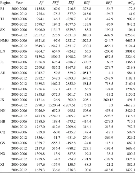
Table 7. The components of the complete decomposition analysis

Region Year P_kt^eff PS_kt^eff EI_kt^eff ES_kt^eff EFkt^eff C_kt

BJ 2000-2006 1155.8 169.0 -716.5 -378.8 -56.7 172.8

2006-2012 725.4 175.2 -877.9 215.0 -196.7 41.0

TJ 2000-2006 994.1 146.3 -228.7 43.8 -47.9 907.6

2006-2012 1678.7 194.2 -1077.6 133.8 -86.9 842.2

SX 2000-2006 5406.0 1134.7 -6329.3 85.3 -190.3 106.4

2006-2012 12357.2 225.9 -5531.8 1810.3 -602.9 8258.6 NMG 2000-2006 6321.8 -97.6 -2321.7 1027.5 -244.7 4685.3 2006-2012 9849.3 -1547.3 -2551.7 230.3 -856.1 5124.4

LN 2000-2006 4204.7 654.9 -924.2 65.5 -200.0 3801.0

2006-2012 5139.2 -1509.2 -1098.2 350.5 -657.5 2224.9

JL 2000-2006 1956.8 625.4 -886.2 -390.2 60.2 1366.1

2006-2012 2769.8 -835.2 -1967.3 92.5 -279.7 -219.8

AH 2000-2006 1042.7 59.8 529.2 -1051.7 4.1 584.1

2006-2012 2832.7 542.3 -3593.3 1643.2 -242.9 1182.1 2000-2012 3689.3 1462.2 -2853.9 581.5 -718.5 2160.4

FJ 2000-2006 1256.4 177.1 -431.9 168.5 124.8 1294.9

2006-2012 1858.8 -572.5 -201.7 78.8 -13.2 1150.2

JX 2000-2006 1131.4 -126.9 -302.0 -205.1 -260.12 491.3 2006-2012 2970.3 3520.94 -1207.51 175.23 3.3 -4612.5 HN 2000-2006 5026.9 -652.8 -995.1 503.6 -453.4 3429.2 2006-2012 4473.8 -2249.3 -805.7 495.7 -598.2 1316.3

HB 2000-2006 1788.6 188.4 -573.2 -414.4 -279.3 710.1

2006-2012 1767.0 -412.6 -2209.6 316.1 -213.5 -752.7

CQ 2000-2006 959.8 -60.0 -435.2 147.4 -12.1 599.9

2006-2012 1356.4 -31.7 -681.9 250.4 -366.9 526.2

GS 2000-2006 1339.7 -555.3 -192.8 -24.0 115.1 682.7

2006-2012 2117.8 516.4 -980.2 227.1 -192.4 1688.6

NX 2000-2006 1309.8 13.9 -587.5 99.3 -35.3 800.2

2006-2012 1739.6 -4.2 -24.9 -191.9 -192.9 1325.8

XJ 2000-2006 997.6 -155.9 150.5 -88.5 -21.2 882.5

2006-2012 1639.3 336.6 -236.3 100.6 -418.0 1422.1

The impact of each single factor is illustrated in the following remarks.

Industrial output effect (see Figure 2): the output effect is the critical

driving factor in the growth of energy-related CO

emissions influencing carbon emissions changes, reflecting the corresponding growth of industrial output in 15 regions. In most regions, the contribution amounts to 60%-70%.

Tianjin shows the highest impact (180.8%), followed by Inner Mongolia and

Ningxia. Among the leading industries contributing to the rise in the

industrial output, chemical, ferrous metals, and the electric industry are predominant in these regions (see Table 5). The output of these three sub- sectors averagely amount to about 60% of the high pollution industries.

Among them, ferrous metals and the electric industry are the largest energy consumers of the seven sub-sectors. Conversely, Liaoning and Anhui present the lowest influence in accordance with the declining role of high pollution industries in their economies.

Figure 2. Percent change in pollution-intensive industrial CO2 emissions due to the output effect

Industrial structure effect (Figure 3): From the perspective of absolute amount, in the period 2000-2012, the industrial structure effect mainly has a positive effect in Jiangxi and Tianjin, in that the share of high CO

emission industries such as ferrous metal, electric and other industries are growing rapidly, leading to the rapid growth of CO

emissions. Unfortunately, no dramatic changes take place in typical regions toward the reduction in number of the energy intensive sectors. Although Inner Mongolia, Henan and Chongqing present a negative industrial structure effect, it does not show great shifts in regional industrial activities, but a slight decline of energy intensive sectors. Simultaneously, the proportion of low CO

emissions industries in these regions is increasing. Industrial structure, therefore, helps to reduce CO

emissions and plays a negative effect. Tianjin, Beijing, Anhui and Shanxi show an opposite trend with the rapid growth of its heavy industries, thus acquiring its overall industrial development.

Energy intensity effect (Figure 4): the energy intensity effect also plays a

key role in inhibiting carbon emissions increase. Results show that in 15

regions, energy efficiency improvements are higher in the seven energy

intensive industries than other industries, especially in the ferrous metals and

chemical industries. Tianjin, Beijing, Shanxi and Inner Mongolia have great

absolute amounts of this effect, and the energy intensities of these regions

show a sharp drop of about 70%, 52%, 51% and 49%, respectively. The only

exception toward improving energy efficiency is recorded in Xinjiang,

exhibiting energy intensity increase, especially in the ferrous metals, electric

and chemical industries.

Figure 3. Percent change in pollution-intensive industrial CO2 emissions due to the industrial structure effect

Figure 4. Percent change in pollution-intensive industrial CO2 emissions due to the energy intensity effect

Energy structural effects (Figure 5): this effect is generally less than 10%. It is dominated by the energy consumption structure of China, and it reflects that China’s fuel switching from coal and oil to natural gas is not obvious, the primary energy type of consumption is still coal. The energy structure in Tianjin, Inner Mongolia and Chongqing, plays a significant positive role, indicating that the adjustment of energy in these areas promotes the carbon emissions increase. The energy structure in Beijing, Anhui, Jilin and Hubei, shows a negative effect. In addition to a positive shift from coal and oil towards natural gas, they further increase the use of biomass and of combined electricity in energy intensive industries.

Figure 5. Percent change in pollution-intensive industrial CO2 emissions due to the energy structure effect

Energy emission intensity effect (Figure 6): the effect of energy

emissions intensity on carbon emissions is relatively small and negative as a

whole, showing that the effect of energy emission intensity on carbon emissions plays a slightly inhibitory role in most regions. It reflects that the gradual implementations of energy-saving policies improve the energy efficiency and decrease the energy intensity in most regions with growing shares of natural gas or renewable energies. Fujian province is the only area showing a rising effect.

Figure 6. Percent change in pollution-intensive industrial CO2 emissions due to the energy emission intensity effect

4.3 Analysis of reduction efforts

Figure 7 presents the emission reduction efforts made during the period 2000-2006 and 2006-2012. It can be observed that the emission reduction measures of 15 regions are basically effective in two periods. The top three are Beijing, Tianjin and Fujian. In the period 2006-2012, their efforts lead to a total emission reduction of about 17%-39%. In the other twelve areas the respective percentage is below 10%. Among them, Shanxi’s reduction effort lead to an accumulated decrease of 17093.6 × 10

ton (i.e. -3.8%) CO

emissions during the period 2000-2012.

It should be noted that this does not mean the efforts in the 15 areas are sufficient. In Beijing, the efforts made in the period 2006-2012 have compensated for a small part of the negative changes of the others. On the one hand, that might be the reason that the marginal cost of further reducing energy intensity or of increasing the share of cleaner energy forms for Beijing’s fuel mix is high. On the other hand, in this period, not all the energy intensity of pollution-intensive industries declined in Beijing. The growth rate of the oil industry and electricity industry reached 127% and 63%, respectively, which makes the overall energy intensity fail to curb the increase of carbon emissions.

Figure 7. Absolute change in pollution-intensive industrial CO2 emissions associated with emission reduction effort

Figures 1 to 7 reveal significant points. For example, Beijing, despite its impressive efforts, failed to decrease carbon emissions below the 2000 level, conversely emissions exhibited an increase of 13%. Similarly, with a total increase of 140%, Tianjin showed great initiatives in promoting CO

emission reduction measures. This indicates that we cannot assess the effort of government’s performance only based on the change of the amount of CO

emissions.

4.4 Analysis of decoupling index

Figures 8 and 9 show the decoupling index calculated for the 15 regions under consideration, together with the distribution of four efforts. It indicates that among the four decoupling indexes, the biggest contributor to the total decoupling index is energy intensity, followed by industry structure and energy structure, while energy emission intensity is the smallest contributor.

Figure 8. The decoupling index of high pollution industries of 15 regions in the period 2000- 2006

Figure 9. The decoupling index of high pollution industries of 15 regions in the period 2006- 2012

According to the decoupling index, in the period 2006-2012, the 15 regions can be divided into three categories:

Regions with a strong decoupling index (D>1), including Beijing: The

decoupling index of Beijing’s pollution-intensive industries has changed

from 0.39 in the period 2000-2006 to 1.48 in the period 2006-2012. From

Figures 1 and 7, we find that the regions with a strong decoupling index is

mainly due to the larger decoupling index of energy intensity, indicating that

carbon emission reductions due to energy intensity reduction are greater than

the increase resulting from industrial growth. At the same time, among the

15 regions, Beijing presents a low and positive industrial output effect, which indicates that its decoupling procession goes along with the stabilization of energy-intensive industries’ production and with shifts toward other sectors. Of course, the fuel switches in utilities in Beijing is also a very important cause.

Regions

with a weak decoupling effect (0<D<1), including Jiangxi, indicate that carbon emission reductions owing to government efforts in their pollution-intensive industries have compensated for a large part of the increases caused by industrial growth. Energy intensity is still the decisive factor to make Jiangxi weak in decoupling, while other factors play a minor role. The industrial structure of Jiangxi plays a negative role in the total decoupling index because the ratio of high pollution industry output to regional output increased during 2000-2012, thus making carbon emissions increased.

Regions with no decoupling effect (D<0) included all regions except Beijing and Jiangxi. Results show that in most regions the carbon emissions reduction measures failed to inhibit the increase of carbon emissions and the industrial output effect on carbon emissions played a positive and dominant role. In fact, the emission reduction measures of these regions are basically effective, but it does not suffice.

4.5 Analysis of reduction potential

The above reflects the government’s carbon emissions reduction efforts.

The results can be used to determine policy priorities for improving the decoupling effectiveness in 15 regions. For example, for regions with no decoupling effect, the possibilities to further reduce energy intensities should be reconsidered. Although most of the 15 regions present no decoupling effect, most governments show great enthusiasm in promoting CO

reduction. So, what can the reduction potential of CO

emissions for the pollution-intensive industries be?

Table 8 shows the carbon emission intensity of 15 regions. In the period 2000-2012, the carbon emissions intensity of Tianjin is the minimum, namely, Tianjin will

as a target region, and the carbon emissions intensity of other regions will gradually converge to Tianjin. The results in descending order are listed in Table 9.

Table 8. The carbon emissions intensity of pollution-intensive industries in the period 2000- 2012

2000 2001 2002 2003 2004 2005 2006 2007 2008 2009 2010 2011 2012 Average BJ 2.7 2.5 3.5 3.3 3.3 3.3 2.8 2.5 2.1 1.9 1.1 1 0.9 2.4 TJ 1.2 1.4 1.2 1.7 0.8 1.2 1.4 1.4 1.2 1.2 0.9 0.8 0.8 1.2 SX 25.4 28.0 31.4 30.9 26.8 25.4 24.3 22.7 19.7 19 17.2 16 14.7 23.2 NMG 16.6 15.8 17.3 17.1 17.9 17.7 16.1 14.9 14.3 12.5 11.2 12.5 11.4 15 LN 6.1 5.6 5.5 5.9 5.7 5.5 5.1 4.7 4 3.5 3.7 3.4 3.1 4.8 JL 7.4 6.9 6.9 6.7 5.8 7.1 6.7 5.5 5.5 4.8 4.5 3.9 3.8 5.8 AH 7.2 8.2 7.2 8.6 8.9 7.8 7.5 7.2 7.1 6.7 6 5.5 5.1 7.2 FJ 3.7 3.5 3.8 3.3 4.6 4.1 4 4.2 3.9 3.7 3.2 3.4 2.9 3.7 JX 6.2 5.7 5.4 6.1 6.6 5.7 5.5 5.1 4.4 4 3.7 3.6 2.9 5 HN 7.2 7.1 6.6 6.4 7.6 7 6.9 6.5 5.8 5.1 4.7 4.4 4 6.1 HB 3.5 3.3 3.5 3.5 3.8 4.6 4.2 3.4 2.8 2.6 2.4 2.2 1.9 3.2 CQ 6.9 6.3 5.8 5.8 5.1 4.9 5 4.8 4 3.6 3.1 3.1 2.4 4.7 GS 5.2 2.2 5.0 5.2 6.2 6 5.6 5.5 5.3 4.5 4.6 4.6 4.2 4.9