Approximation of Center Manifolds on the Renormalization Group Method
Department of Applied Mathematics and Physics Kyoto University, Kyoto, 606-8501, Japan
Hayato CHIBA∗1 Apr/27/2008
Abstract
The renormalization group (RG) method for differential equations is one of the perturbation methods for obtaining approximate solutions. This article shows that the RG method is effectual for obtaining an approximate center manifold and an approximate flow on it, when applied to equations having a center manifold.
1 Introduction
The renormalization group (RG) method of Chen, Goldenfeld and Oono [2,3] is one of the perturba- tion methods for obtaining solutions which are approximate to exact solutions for a long time interval.
Over the last decade, various methods and techniques for deriving RG equations and approximate solutions have been studied by many authors [2,3,4,5,6,7,9,11,12,13,15]. Kunihiro [11,12] showed that an approximate solution obtained by the RG method is an envelope of a family of curves which are constructed by the naive expansion. Ziane [15] and DeVilleet al. [6] defined the first order RG equation by using an averaging operator and they proved that an exact solution of a given equation and an approximate solution obtained by the RG method are sufficiently close to each other for a long time interval. Chiba [4,5] defined the higher order RG equation on the idea of Kunihiro, Ziane, and DeVilleet al. to obtain higher order approximate solutions. He also proved that if the RG equation has a normally hyperbolic invariant manifoldN, the original equation also has an invariant manifold which is diffeomorphic toN.
It has been shown that the RG method covers the traditional singular perturbation methods, such as the multi-scaling method [2,3], the boundary layer theory [2,3], the averaging method [6], the normal form theory [5,6]. In particular, Chen, Goldenfeld, Oono [3] and Ei, Fujii, Kunihiro [7] applied the RG method to an equation whose linear part has eigenvalues on the left half plane and the imaginary axis to construct an approximate center manifold, while many authors had studied the case that all eigenvalues of the linear part lie on the imaginary axis.
This paper offers a rigorous proof of the fact that the RG method provides an approximate center
∗1E mail address : [email protected]
manifold, and further the RG method is improved to raise accuracy of approximation by using the higher order RG equation. An approximate flow on an approximate center manifold is derived as well. Moreover, it is shown that if the RG equation has a normally hyperbolic invariant manifold, a given equation also has an invariant manifold on the center manifold. This method for obtaining an approximate center manifold and a flow on it is called therestricted RG methodbecause a domain of the RG equation is restricted to a center subspace of an unperturbed part of a given equation.
This paper is organized as follows: Sec.2 presents basic facts and definitions in dynamical systems.
In Sec.3, the restricted RG method is proposed and main theorems on the restricted RG method are proved. Sec.4 presents a few examples.
2 Basic facts
Let f be a time independentCr vector field on aCr manifold M andϕ : R× M → M its flow, which satisfiesϕt ◦ϕs = ϕt+s, ϕ0 = idM, whereidM denotes the identity map ofM. For fixedt ∈R, ϕt :M→ Mdefines a diffeomorphism ofM. We denote byϕt(x0)≡ x(t), t∈R, a solution of the ODE
˙
x= f(x) through x0∈Matt=0. We assumeϕtis defined for∀t∈R.
For a time-dependent vector field, letx(t, τ, ξ) denote a solution of an ODE ˙x(t)= f(t,x) throughξat t=τ, which defines a flowϕ:R×R×M→Mbyϕt,τ(ξ)= x(t, τ, ξ). For fixedt, τ∈R,ϕt,τ:M→M is a diffeomorphism ofMsatisfying
ϕt,t◦ϕt,τ =ϕt,τ, ϕt,t =idM. (2.1) Conversely, a family of diffeomorphismsϕt,τ of M, which isC1 with respect totandτ, satisfying the above equality for∀t, τ∈Rdefines a time dependent vector field onMthrough
f(t,x)= d
dττ=tϕτ,t(x). (2.2)
Theorem 2.1. (Fenichel, [8])
LetMbe aCr manifold (r ≥ 1), andXr(M) the set ofCr vector fields on MwithC1topology. Let f be aCr vector field on M and suppose that N ⊂ M is a compact connected normally hyperbolic f-invariant manifold. Then, there is a neighborhoodU ⊂ Xr(M) of f s.t. for∀g ∈ U, there exists an unique normally hyperbolicg-invariantCr manifoldNg ⊂ MnearN. In particular ifg∈ Uis within anO(ε) neighborhood of f,Nglies within anO(ε) neighborhood ofNas well.
See [8],[10],[14] for the proof of Thm.2.1 and the definition of normal hyperbolicity.
Definition 2.2. Letϕt be the flow of a vector field on a manifold M. A manifold N ⊂ Mis called a locally invariant manifoldif there exists a numberT =T(x)>0 for eachx∈Nsuch that{ϕt(x)| −T <
t<T} ⊂N.
Theorem 2.3. (Center Manifolds Theorem) Consider the system x˙= Ax+ f(x,y), x∈Rn,
˙
y= By+g(x,y), y∈Rm, (2.3)
whereAandBare constant matrices such that all eigenvalues ofAlie on the imaginary axis and all eigenvalues of Blie on the left half plane. Suppose that f andg areC2 vector fields which vanish together with their derivatives at the origin. Then, there exists an n-dimensional locally invariant manifold which is tangent to thex-plane at the origin. It is called alocal center manifold.
See Carr [1] for the proof of Thm.2.3.
3 Restricted Renormalization Group Method
In this section, we propose the restricted RG method for obtaining a center manifold and a flow on it approximately.
LetF be ann×nmatrix all of whose eigenvalues lie on the imaginary axis or the left half plane.
We assume that at least one eigenvalue is on the imaginary axis because if all eigenvalues lie on the left half plane, the origin remains to be a stable fixed point of the equation under small perturbation and topological properties of the flow near the origin is trivial. Further, we suppose that the Jordan block corresponding to the eigenvalues on the imaginary axis is semisimple. Letg(t,x, ε) be a time- dependent vector field onRnwhich isC∞class with respect tot,xandε ∈ R. Letg(t,x, ε) admit a formal power series expansion inε,g(t,x, ε) =g1(t,x)+εg2(t,x)+ε2g3(t,x)+· · ·. We suppose that gi(t,x)’s are periodic intand polynomial in x, whose degrees are equal to or larger than 1, although the results in this section still hold even ifgi(t,x)’s are almost periodic int ∈Ras long as the set of Fourier exponents ofgi(t,x)’s has no accumulation points (see Chiba [4]).
Consider an ODE
˙
x=F x+εg(t,x, ε)
=F x+εg1(t,x)+ε2g2(t,x)+· · ·, x∈Rn, (3.1) whereε∈Ris a small parameter. Replacingxin (3.1) byx= x0+εx1+ε2x2+· · ·, we rewrite (3.1) as
˙
x0+εx˙1+ε2x˙2+· · ·=F(x0+εx1+ε2x2+· · ·)+∞
i=1
εigi(t,x0+εx1+ε2x2+· · ·). (3.2) Expanding the right hand side of the above equation with respect toεand equating the coefficients of
eachεiof the both sides, we obtain ODEs forx0,x1,x2,· · · as
˙
x0= F x0, (3.3)
˙
x1= F x1+G1(t,x0), (3.4)
...
˙
xi= F xi+Gi(t,x0,x1,· · · ,xi−1), (3.5) ...
where the inhomogeneous termGiis a smooth function oft,x0,x1,· · ·,xi−1. For instance,G1,G2and G3are given by
G1(t,x0)=g1(t,x0), (3.6)
G2(t,x0,x1)= ∂g1
∂x(t,x0)x1+g2(t,x0), (3.7)
G3(t,x0,x1,x2)= 1 2
∂2g1
∂x2 (t,x0)x21+ ∂g1
∂x (t,x0)x2+ ∂g2
∂x(t,x0)x1+g3(t,x0), (3.8) respectively. We denote byX(t) =eFtthe fundamental matrix of the unperturbed equation ˙x0 = F x0. LetN0be the center subspace, which is a hyperplane inRnspanned by the eigenvectors ofFassociated with eigenvalues on the imaginary axis. Note that ifA∈N0, thenX(t)A∈N0for allt∈R.
Define functionsRi :N0 →Rnandh(i)t :N0→Rnwithi=1,2,· · · by R1(A) := lim
t→−∞
1 t
t
X(s)−1g1(s,X(s)A)ds, (3.9) h(1)t (A) :=X(t)
t
X(s)−1g1(s,X(s)A)−R1(A)
ds, (3.10)
and
Ri(A) := lim
t→−∞
1 t
t
X(s)−1Gi(s,X(s)A,h(1)s (A),· · ·,h(is−1)(A))
−X(s)−1
i−1
k=1
(Dh(k)s )ARi−k(A)
ds, (3.11)
h(i)t (A) :=X(t)
t
X(s)−1Gi(s,X(s)A,h(1)s (A),· · ·,h(is−1)(A))
−X(s)−1
i−1
k=1
(Dh(k)s )ARi−k(A)−Ri(A)
ds, (3.12)
fori = 2,3,· · ·, where (Dh(k)t )A denotes the derivative ofh(k)t (A) with respect to A ∈ Rn. Note that h(k)t (A) is differentiable as a function onRn. Integral constants of the indefinite integrals of the above equations are taken to be zero. What this means is as follows: Sincegi(t,x) is a polynomial inxand since it can be expanded into the Fourier series with respect tot, it is easy to see that each integrand in Eqs.(3.9) to (3.12) can be written as a linear combination of functions of forms eξs, ξ ∈ C. In
particular, the integrand in Eq.(3.10) does not have a constant term because if the Fourier series of X(s)−1g1(s,X(s)A) has a constant term with respect tot, it has to be equal to the termR1(A). Therefore we can take the integral constant of the indefinite integralt
(X(s)−1g1(s,X(s)A)−R1(A))dsto be zero so that the indefinite integral is written as a linear combination of functions of formseξt, ξ0. Func- tionsh(i)t (A), i= 2,3,· · · are defined in a similar way so thatX(t)−1h(i)t (A) are linear combinations of functions of formseξt, ξ0. Note thatRi(A)’s are independent of integral constants in Eqs(3.9),(3.11).
Lemma 3.1. FunctionsR1(A),R2(A),· · · are well defined and (i) eachRi(A) satisfiesRi(A)∈N0,
(ii) eachh(i)t (A) is bounded uniformly int∈R.
Proof. We can assume thatFis of the form
F =
λ1
...
0
λl
0 S
,
where eigenvalues λ1,· · ·, λl lie on the imaginary axis and eigenvalues λl+1,· · ·, λn of S lie on the left half plane with Re(λl+1) ≥ · · · ≥ Re(λn). Let πc and πs be the projections from Rn onto the center subspace N0 = {(x1,· · · ,xl,0,· · ·0)|xi ∈ R} and its complementary subspace N0⊥ := {(0,· · ·0,xl+1,· · ·,xn)|xi ∈R}, respectively. Sinceg1(t,x) andX(t)AwithA∈N0are bounded int ∈ R, there exists a positive constantC such that||g1(t,X(t)A)|| ≤ Cfor each A ∈ N0. Since the integrand X(s)−1g1(s,X(s)A) in Eq.(3.9) is bounded in s ≤ 0, it is easy to verify that the limit in Eq.(3.9) converges andR1(A) is well-defined.
To prove the lemma (i) fori= 1, note that there exist positive constantsD, δsuch that||πsX(t)−1|| ≤ De−Re(λl+1)t−δt fort≤0 and−Re(λl+1)−δ >0. Then,πsR1(A) proves to satisfy
||πsR1(A)|| ≤ lim
t→−∞
1
−t
t
||πsX(s)−1g1(s,X(s)A)||ds
≤ lim
t→−∞
1
−t
t
CDe−Re(λl+1)s−δsds=0.
This means thatR1(A)∈N0. Next, to prove (ii) of the lemma, we evaluate||πsh(1)t (A)||to get
||πsh(1)t (A)|| ≤
t
||πsX(t−s)g1(s,X(s)A)−πsX(t)R1(A)||ds≤
t
CDeRe(λl+1)(t−s)+δ(t−s)ds. (3.13) Since the integral constant is equal to zero, we obtain||πsh(1)t (A)|| ≤ −CD/(Re(λl+1)+δ). On the other hand,πch(1)t (A) satisfies
πch(1)t (A)=πcX(t)
t
πcX(s)−1g1(s,X(s)A)−R1(A)
ds. (3.14)
Then, the boundedness of theπch(1)t (A) results from Prop.A.4 of Chiba[4], in which the boundedness of h(i)t (A),i=1,2,· · · is proved for the case that all eigenvalues ofFlie on the imaginary axis. Therefore h(1)t (A)=πsh(1)t (A)+πch(1)t (A) is bounded uniformly int∈R.
Lemma 3.1 forRi(A),h(i)t (A),i=2,3,· · · is also proved by induction in the same manner as above.
By Lemma 3.1 (i), eachRi(A) defines a vector field onN0.
Definition 3.2. Along with R1(A),· · ·,Rm(A) given by Eqs.(3.9),(3.11), we define the m-th order restricted RG equationfor Eq.(3.1) to be
A˙=εR1(A)+ε2R2(A)+· · ·+εmRm(A), A∈N0. (3.15) Using h(1)t (A),· · ·,h(m)t (A) given by Eqs.(3.10),(3.12), we define the m-th order RG transformation αt :N0 →Rnby
αt(A)= X(t)A+εh(1)t (A)+· · ·+εmh(m)t (A). (3.16)
Remark 3.3. A few remarks are in order. WhileRi(A)∈N0 ⊂Rnis ann-dimensional vector, as many as dimN0component equations in Eq.(3.15) are independent of one other. Thus we regard Eq.(3.15) as a dimN0-dimensional differential equation. Since X(t) is nonsingular andh(1)t (A),· · ·,h(m)t (A) are bounded uniformly in t ∈ R, for sufficiently small |ε|, there exists an open set U = U(ε) ⊂ N0
including the origin such thatU is compact and the restriction of αt toU is diffeomorphism fromU intoRn. It is easy to verify thatαt(0)=0, thusαt(U) includes the origin.
Now we are in a position to state fundamental results of our restricted RG method.
Theorem 3.4. (Approximation of Orbits)
LetA=A(t) be a solution to them-th order restricted RG equation (3.15). Define the curvex(t) by x(t)=αt(A(t))= X(t)A(t)+εh(1)t (A(t))+· · ·+εmh(m)t (A(t)). (3.17) Then, there exist positive constants ε0,C,T and a compact subset V = V(ε) ⊂ α0(N0) including the origin such that for∀|ε| < ε0, every solution x(t) of Eq.(3.1) andx(t) defined by Eq.(3.17) with x(0)=x(0)∈V satisfy the inequality
||x(t)−x(t)||<Cεm, (3.18)
for 0≤t≤T/ε.
Theorem 3.5. (Approximation of Vector Fields)
LetϕRGt be the flow of them-th order restricted RG equation for Eq.(3.1) andαt them-th order RG transformation. Then, there exists a positive constantε0such that the following holds for∀|ε|< ε0: (i) A map
Φt,t0 :=αt◦ϕRGt−t0 ◦α−t01 :αt0(U)→Rn (3.19)
defines a local flow onαt0(U) for eacht0∈R, whereU = U(ε) ⊂ N0is an open set on whichαt0 is a diffeomorphism (see Rem.3.3). TheΦt,t0induces a time-dependent vector fieldFεthrough
Fε(t,x) := d
daa=tΦa,t(x), x∈αt(U), (3.20) whose integral curves are the approximate solutionsx(t) defined by Eq.(3.17).
(ii) There exists a time-dependent vector fieldFε(t,x) such that
Fε(t,x)= F x+εg1(t,x)+· · ·+εmgm(t,x)+εm+1Fε(t,x), x∈αt(U) (3.21) where Fε(t,x) is C∞ class with respect to t,x andε. In particular, Fε(t,x) and its derivatives are bounded uniformly int∈R.
Theorem 3.4 and Theorem 3.5 are proved in the same manner as in Thm.A.8 and Thm.A.6 of Chiba[4], respectively, in which the theorems are proved for the case that all eigenvalues of F lie on the imaginary axis.
The following two theorems are concerned with an autonomous equation
˙
x= F x+εg1(x)+ε2g2(x)+· · ·, x∈Rn, (3.22) whereε∈Ris a small parameter. Like Eq.(3.1),Fis ann×nmatrix all of whose eigenvalues lie on the left half plane or the imaginary axis, and the Jordan block corresponding to the eigenvalues on the imaginary axis is semisimple. Furthergi(x)’s are polynomial vector fields on Rnwhose degrees are equal to or larger than 1.
Theorem 3.6. (Inheritance of the Symmetries)
(i) Suppose that a Lie groupGacts on the center subspace N0 spanned by eigenvectors ofF asso- ciated with eigenvalues on the imaginary axis. If vector fieldsF xandg1(x),g2(x),· · ·,are invariant under the action ofG, then them-th order restricted RG equation for Eq.(3.22) is also invariant under the action ofG.
(ii) Them-th order restricted RG equation commutes with the linear vector fieldF xwith respect to Lie bracket product. Equivalently, eachRi(A), i=1,2,· · · satisfies
X(t)Ri(A)=Ri(X(t)A), A∈N0. (3.23)
Theorem 3.7. (Existence of Invariant Manifolds)
LetεkRk(A) be a first non-zero term in the RG equation (3.15). If the vector fieldεkRk(A) onN0has a compact normally hyperbolic invariant manifoldM0⊂ N0, then the original equation (3.22) also has a normally hyperbolic invariant manifoldMε, which is diffeomorphic toM0, for sufficiently small|ε|. In particular, the stability ofMεand ofM0coincide.
Theorem 3.6 and Theorem 3.7 are proved in the same manner as in Thm.A.9 and Thm.A.7 of Chiba[4], respectively, in which the theorems are proved for the case that all eigenvalues of F lie on the imaginary axis.
If degrees of polynomialsgi(x)’s in Eq.(3.22) are equal to or larger than 2, Eq.(3.22) has a dimN0- dimensional local center manifold tangent toN0at the origin. Ifgi(x)’s have linear parts, Eq.(3.22) no longer has a dimN0-dimensional center manifold because the linear part of right hand side of Eq.(3.22) no longer has dimN0eigenvalues on the imaginary axis in general. However, even in this case, there exists a locally invariant manifold which is diffeomorphic to a dimN0-dimensional closed ball. This fact is explained as follows: Recall thatN0is a normally hyperbolic invariant hyperplane of the vector fieldF x. Fix ann-dimensional closed ballKincluding the origin. We can perturb the vector fieldF xin a small neighborhood of the boundary ofKso thatN0∩Kis a normally hyperbolic invariant manifold of the resultant perturbed vector field, sayF x+h(x). Ifε >0 is sufficiently small, by Thm.2.1, a vector fieldF x+h(x)+εg1(x)+· · · has a normally hyperbolic invariant manifoldNεwhich is diffeomorphic toN0∩K. Sinceh(x) has its support in a small neighborhood of the boundary ofK, Eq.(3.22) hasNε as a locally invariant manifold. In what follows, a locally invariant manifold in the above sense is also called a center manifold.
t K
N0
N0
Nǭ
ǩ( )
Fig. 1: A center subspaceN0, a center manifoldNε, and an approximate center manifoldαt(N0).
Now our purpose is to construct a center manifold of Eq.(3.22) approximately. Before showing the main theorem, we need a lemma.
Lemma 3.8. The set αt(N0) := {αt(A)|A ∈ N0} is independent oft∈ R, whereαt is them-th order RG transformation for Eq.(3.22).
Proof. At first, we prove that h(i)t+t(A) = h(i)t (X(t)A) hold fori = 1,2,· · · and ∀t ∈ R. Since
Ri(X(t)A)= X(t)Ri(A) holds by Thm.3.6 (ii),h(1)t (X(t)A) is calculated as h(1)t (X(t)A)=X(t)
t
X(s)−1G1(X(s)X(t)A)−R1(X(t)A) ds
=X(t)X(t)
t
X(t)−1X(s)−1G1(X(s)X(t)A)−R1(A) ds
=X(t+t)
t
X(s+t)−1G1(X(s+t)A)−R1(A) ds.
By puttings+t= s, the above equation results in h(1)t (X(t)A)=X(t+t)
t+t
X(s)−1G1(X(s)A)−R1(A)
ds=h(1)t+t(A). (3.24) The equalitiesh(i)t+t(A)=h(i)t (X(t)A) fori=2,3,· · · are proved in a similar manner by induction. Since X(t) is a diffeomorphism onN0, we obtainh(i)t+t(N0)=h(i)t (N0) and this provesαt+t(N0)=αt(N0).
Theorem 3.9. (Approximation of Center Manifolds)
Letαtbe them-th order RG transformation for Eq.(3.22) andW⊂Ube a compact subset including the origin, whereU ⊂N0is an open set on whichαtis a diffeomorphism (see Rem.3.3). Then, the set αt(W) lies within anO(εm+1) neighborhood of a center manifoldNεof Eq.(3.22).
Proof. By Thm.3.5, the approximate vector field Fεdefined onαt(U) isC1 close to the restriction of the original vector fieldF x+εg1(x)+· · · toαt(U) within anO(εm+1). LetK be ann-dimensional closed ball includingW and αt(W). We can extend Fε to a vector field Fε defined on K such that Fε|K∩αt(U) = Fε|K∩αt(U)andFε isC1close to the original vector fieldF x+εg1(x)+· · · on K within anO(εm+1). Sinceαt(W) is a locally invariant manifold ofFε, our theorem immediately follows from
Thm.2.1.
The present method for obtaining an approximate center manifold and an approximate flow on the manifold defined by Eq.(3.19) is called therestricted RG methodbecause the domain of the RG equa- tion and the RG transformation are restricted toN0.
4 Examples
In this section, we show two simple examples of the restricted RG method.
Example 3.10. Consider the system onR3, d
dt
x y z
=
0 1 0
−1 0 0
0 0 −1
x y z
+ε
yz2
−x3 y2+xz
. (4.1)
A general solution of the unperturbed part is given by
x0
y0
z0
=
Acost+Bsint
−Asint+Bcost Ce−t
=
peit+pe−it ipeit−ipe−it
Ce−t
, (4.2)
where (A,B,C)∈R3is an initial value andpis defined by p=A/2+B/(2i). Introducing the complex variable p makes it simple to work with the RG equation. The center subspace for the unperturbed equation is expressed asN0={(A,B,0)|A,B∈R}. The first order restricted RG equation and the first order RG transformation for Eq.(4.1) are given by
d dt
p
p
= 3iε 2
p|p|2
−p|p|2
, p∈C, (4.3)
αt(A,B)=
cost sint 0
−sint cost 0
0 0 e−t
A B 0
+ε
p3
8 e3it− 3
4|p|2peit+ p3
8 e−3it− 3
4|p|2pe−it i
3p3 8 e3it+ 3
4|p|2peit− 3p3
8 e−3it− 3
4|p|2pe−it
−p2
1+2ie2it+2|p|2+ −p2 1−2ie−2it
, (4.4)
respectively. Therefore, an approximate center manifold of Eq.(4.1) is expressed as
α0(N0)={(A,B, εϕ(A,B)}, (4.5)
ϕ(A,B) := −p2
1+2i+2|p|2+ −p2 1−2i = 2
5A2+ 3 5B2+ 2
5AB. (4.6)
Equivalently, the approximate center manifold is expressed as the graph of the functionz = ε2 5x2+ ε3
5y2+ε2
5xyin (x,y,z) space. This result coincides with an approximate center manifold obtained by a method in [1]. The restricted RG equation (4.3) is solved as
p(t)= 1 2aexpi
3ε 8 a2t+θ
,
wherea, θare arbitrary constants. With this p(t), an approximate solution defined by Eq.(3.17) on the center manifold of (4.1) is given by
x(t)=acos 3ε
8 a2t+t+θ
+ εa3 32 cos
9ε
8 a2t+3t+3θ
− 3εa3 16 cos
3ε
8 a2t+t+θ
, y(t)=−asin
3ε
8 a2t+t+θ
− 3εa3 32 sin
9ε
8 a2t+3t+3θ
− 3εa3 16 sin
3ε
8 a2t+t+θ
, z(t)= εa2
2 − εa2 10 cos
3ε
4 a2t+2t+2θ
− εa2 5 sin
3ε
4 a2t+2t+2θ
.
0 0.01 0.02 0.03 0.04 0.05
-1 -0.5 0 0.5 1
-0.8 -0.4
0 0.4
0.8 -1
0 1 0
1 2 3
x
y
z z
x
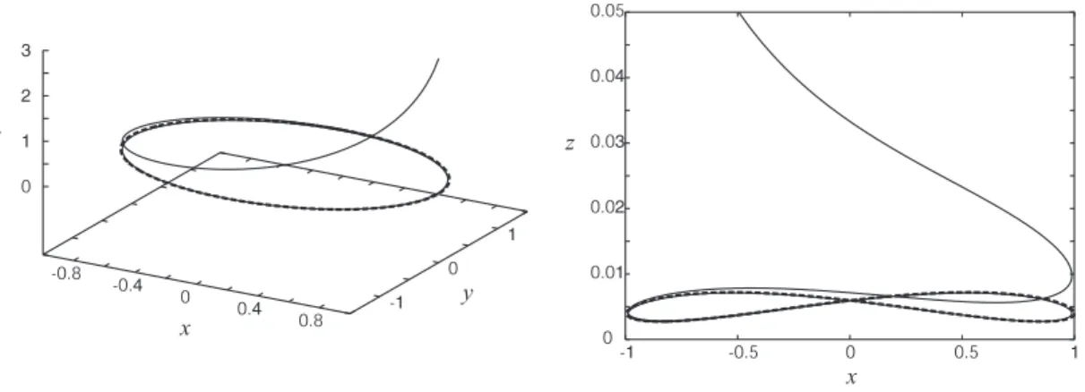
Fig. 2: An exact solution (solid line) to Eq.(4.1) and the approximate solution on the center mani- fold (dashed line).
Numerical observation forε = 0.01 is presented in Fig.2. The solid line denotes an exact solution to Eq.(4.1) with initial value (x,y,z) = (1,0,3), which is out of the center manifold, and dashed line denotes the above-stated approximate solution witha=1, θ=0 on the approximate center manifold.
Example 3.11. We can show that the Hopf bifurcation occurs in the Lorenz equations by applying Thm 3.7. Consider the Lorenz equations
˙
x=−10x+10y,
˙
y=ρx−y−xz,
˙ z=−8
3z+xy,
(4.7)
whereρ∈Ris a parameter. This system has three fixed points:
(0,0,0), (a(ρ),a(ρ), ρ−1), (−a(ρ),−a(ρ), ρ−1), (4.8) wherea(ρ)=
8
3(ρ−1). To show the presence of a bifurcation from the fixed point (a(ρ),a(ρ), ρ−1), we change the coordinate byx→x+a(ρ), y→y+a(ρ), z→z+(ρ−1). Then the system is rewritten
as
˙
x=−10x+10y,
˙
y= x−y−a(ρ)z−xz,
˙
z=a(ρ)x+a(ρ)y− 8 3z+xy.
(4.9) Whenρ=ρ0:=470/19, the derivative of the right hand side of the above system at the origin has the eigenvalues
α=−41
3 , ±β=±4
110
19 i. (4.10)
This means that the origin is not hyperbolic fixed point, so that the Hopf bifurcation may occur. Since we are interested in the behavior of the system near the origin and near the value of the parameter a:=a(ρ0)=
8/3(ρ0−1), we change the coordinates by
x=εX, y=εY, z=εZ, (4.11)
and put
a(ρ)=a−ε2, a=
8/3(ρ0−1)=
3608/57. (4.12)
Substituting (4.11),(4.12) into the system (4.9), we obtain d
dt
X Y Z
=
−10 10 0
1 −1 −a
a a −8/3
X Y Z
+ε
0
−XZ XY
−ε2
0
−Z X+Y
. (4.13)
Further, we change the coordinate so that the matrix in the right hand side of the above is brought into the diagonal matrix diag (β,−β, α). Then, the center subspace of the unperturbed equation of the resultant system is expressed asN0={(X,Y,0)|X,Y ∈R}and the second order restricted RG equation for the system is given by
A˙/ε2=−38√
51414A
47779 + 91438888520A2B
18481807848339 −i2086√ 615A 47779 −i
714354199417
190 11 A2B 55445423545017 , B˙/ε2=−38√
51414B
47779 + 91438888520AB2
18481807848339 +i2086√ 615B 47779 +i
714354199417
190
11 AB2 55445423545017 .
(4.14) Note that the first order restricted RG equationR1vanishes. On puttingA=reiθandB=A, Eq.(4.14) is brought into
˙
r=−ε2p1r+ε2p2r3, θ˙ =−ε2q1−ε2q2θ2, p1= 38√
51414
47779 ,p2= 91438888520
18481807848339,q1= 2086√ 615
47779 ,q2= 714354199417
190
11
55445423545017 .
(4.15)
The equation ofr has two fixed pointsr = 0 andr = r0 :=
p1/p2, and it is easy to show that the fixed pointr0is unstable. This proves that the RG equation (4.14) has an unstable normally hyperbolic invariant circle. By Thm.3.7, the equation (4.9) also has an unstable periodic orbit ifa(ρ) is slightly smaller thana= √
3608/57.
Acknowledgment
The author would like to thank Professor Toshihiro Iwai for critical reading of the manuscript and for useful comments. The author is also grateful to Assistant Professor Yoshiyuki Y. Yamaguchi for bringing his attention to the RG method.
Reference
[1] J. Carr, Applications of Centre Manifold Theory, Springer-Verlag, 1981
[2] L. Y. Chen, N. Goldenfeld, Y. Oono, Renormalization group theory for global asymptotic anal- ysis, Phys. Rev. Lett. 73 (1994), no. 10, 1311-15
[3] L. Y. Chen, N .Goldenfeld, Y. Oono, Renormalization group and singular perturbations: Mul- tiple scales, boundary layers, and reductive perturbation theory, Phys. Rev. E 54, (1996), 376-394
[4] H. Chiba, C1 approximation of vector fields based on the renormalization group method, (to appear)
[5] H. Chiba, Simplified Renormalization Group Equations for Ordinary Differential Equations, (to appear)
[6] R. E. Lee DeVille, A. Harkin, M. Holzer, K. Josi´c, T. Kaper, Analysis of a renormalization group method and normal form theory for perturbed ordinary differential equations, Physica D, (preprint)
[7] S. Ei, K. Fujii, T. Kunihiro, Renormalization-group method for reduction of evolution equa- tions; invariant manifolds and envelopes, Ann. Physics 280 (2000), no. 2, 236-298
[8] N. Fenichel, Persistence and smoothness of invariant manifolds for flows, Indiana Univ. Math.
J. 21 (1971), 193-226
[9] S. Goto, Y. Masutomi, K. Nozaki, Lie-Group Approach to Perturbative Renormalization Group Method, Prog. Theor. Phys. vol.102, No.3. (1999),pp. 471-497.
[10] M. W. Hirsch, C. C. Pugh, M. Shub, Invariant manifolds, Springer-Verlag, (1977) Lec, notes in math. 583
[11] T. Kunihiro, A geometrical formulation of the renormalization group method for global analy- sis, Progr. Theoret. Phys. 94 (1995), no. 4, 503-514
[12] T. Kunihiro, The renormalization-group method applied to asymptotic analysis of vector fields, Progr. Theoret. Phys. 97 (1997), no. 2, 179-200
[13] K. Nozaki, Y. Oono, Renormalization-group theoretical reduction, Phys. Rev. E, 63, 046101 (2001)
[14] S. Wiggins, Normally hyperbolic invariant manifolds in dynamical systems , Springer-Verlag , (1994)
[15] M. Ziane, On a certain renormalization group method, J. Math. Phys. 41 (2000), no. 5, 3290- 3299