Signatures of Novel Spin Liquids in Kagome‑like Lattices
Author Rico Pohle
Degree Conferral Date
2017‑12‑07
Degree Doctor of Philosophy Degree Referral
Number
38005甲第8号 Copyright
Information
(C) 2017 The Author
URL http://doi.org/10.15102/1394.00000173
Okinawa Institute of Science and Technology Graduate University
Thesis submitted for the degree
Doctor of Philosophy
Signatures of Novel Spin Liquids in Kagome-like Lattices
by
Rico Pohle
Supervisor: Nic Shannon
November, 2017
Declaration of Original and Sole Authorship
I, Rico Pohle, declare that this thesis entitled Signatures of Novel Spin Liquids in Kagome-like Lattices and the data presented in it are original and my own work.
I confirm that:
• This work was done solely while a candidate for the research degree at the Oki- nawa Institute of Science and Technology Graduate University, Japan.
• No part of this work has previously been submitted for a degree at this or any other university.
• References to the work of others have been clearly attributed. Quotations from the work of others have been clearly indicated, and attributed to them.
• In cases where others have contributed to part of this work, such contribution has been clearly acknowledged and distinguished from my own work.
• None of this work has been previously published elsewhere, with the exception of the following: Chapter 4 has been published in collaboration with Owen Benton and Ludovic Jaubert in [1].
Date: November, 2017 Signature:
iii
Abstract
Signatures of Novel Spin Liquids in Kagome-like Lattices
The phenomenon of magnetism in solids aroused the curiosity of scientists already in ancient times. While quantum mechanical effects on a single–particle level are well understood, magnets offer phenomena caused by collective interactions between many electrons and provide the opportunity to find novel states of matter. In this context, frustrated magnets play a central role, since interactions between local magnetic mo- ments on a crystallographic lattice cannot be satisfied at the same time. This can prevent the systems to order even at very low temperatures, creating a magnetic state similar to those of liquids, which gives them the namespin liquids. Within this field, the kagome lattice — a two–dimensional network of corner–sharing triangles — has played a particularly iconic role and continues to provide rich inspiration to theoreticians and experimentalists alike.
In this thesis, we first explore the thermodynamic properties and signatures of classi- cal spin liquids on kagome–like lattices, by the use of complementary analytical Husimi tree and numerical Monte Carlo simulation techniques. The emerging phenomenon of aCurie–law crossover, reflecting a crossover between a high–temperature paramagnet and a low–temperature collective paramagnet, turns out to be a powerful signature of exotic physics in classical spin liquids, and explains the difficulty of making a precise estimate of the Curie–Weiss temperature in experiments.
But spin liquids do not necessarily need to show just one Curie–law crossover. The anisotropic Ising model on theshuriken, or square–kagome lattice, shows a succession of multiple Curie–law crossovers due to a rich phase diagram with many disordered ground states. Hereby, low–and high–temperature regimes are less correlated than the intervening classical spin liquid, allowing to extend the definition of reentrant phenom- ena to disordered systems.
Furthermore, we also study dynamical properties of the nearest–neighbour Heisen- berg model on the bilayer breathing kagome lattice, which has been motivated by recent experiments on Ca10Cr7O28. Using semi–classical molecular–dynamics simulations, we are able to reproduce many features seen by inelastic neutron scattering experiments and provide a first explanation of its spin–liquid origin. Surprisingly, we find that ex- citations encode not one, but two distinct types of spin liquids at different time scales.
Fast fluctuations reveal aCoulombic spin liquid, as known from the classical kagome–
lattice antiferromagnet, while slow fluctuations reveal a spiral spin liquid, which can be understood by a mapping onto an effective spin-3/2 honeycomb model.
v
Acknowledgment
I am very honoured and pleased to be one of the first PhD students of the Okinawa Institute of Science and Technology Graduate University (OIST) and want to express my sincere gratitude to all people involved in its past and present development, allowing me to do my doctoral studies on this very special island.
My PhD studies would have never reached to this point without the support of many people. Firstly, I would like show my deep appreciation to Nic Shannon for his continuous support since the first time we met at the “Paul Rackwitz”, a very nice, local restaurant in Dresden–Plauen. While talking about OIST, I would have never thought to do a PhD in theoretical physics in my near future. However, his optimism, love for physics, and engagement for a deep understanding of “everything”
were exceptionally inspiring from the first time we met until the end of my PhD.
Secondly, I would like to thankLudovic Jaubert, for his valuable supervision, since my lab–rotation in the TQM unit at OIST. Next to providing me with all fundamental secrets of Monte Carlo simulations and statistical mechanics, and not–forgettable times late at night in the office, where “short questions” easily expanded into very interesting multiple–hour discussions, I enjoyed his enthusiasm, positivity and pedagogical know–
how. Thirdly, I want to thankMathieu Taillefumierfor teaching me everything I know about high–performance programming and molecular dynamics simulations. Even at very busy times he was available and happy to help out, by convincing my computer code to work as intended. I also want to thank Han Yan, who initiated the work on the Ca10Cr7O28 project (Chapter 5), by brilliantly spotting the connection between different underlying spin–liquid models for this material.
Personally, I want to deeply thank the members of the OIST Karate Club for their continuous support over the last 5 years, enabling me to practice and improve my physical and pedagogical karate skills. Especially I want to thank Kimberly Remund, who basically attended the Karate practice more often than I did, and gave me the secure feeling, that there will be definitely, at any time, at least one student waiting for me in the Dojo. I am in deep dept to my parents and my family back home in Germany, who supported me throughout my whole life and never pushed or criticised me on any of my decisions, as well as my “new” family here in Okinawa, who included me from the first day we met as their “Uchinaa Muukuu” (Okinawan son). Last but not least, I want to thank my wifeYuno Pohle Kaneshi. I would have not been able to finish my studies without her support from the first day I arrived at OIST — while she was working for the Graduate School — until the end of my thesis. Her optimism and attitude to learn and improve herself every day is highly inspiring and encouraging, and allows me to look into a bright future of whatever might await on our way.
vii
Contents
Declaration of Original and Sole Authorship iii
Abstract v
Acknowledgment vii
Contents ix
List of Figures xiii
List of Tables xv
1 Introduction to Magnetism and Spin Liquids 1
1.1 Origin of Magnetism in solids . . . . 1
1.1.1 A historical summary . . . . 2
1.1.2 Hubbard model . . . . 3
1.1.3 Mott insulators . . . . 4
1.1.4 Heisenberg model . . . . 6
1.1.5 Anisotropic exchange . . . . 7
1.2 Magnetic order in conventional magnets . . . . 8
1.2.1 Mean–field theory . . . . 8
1.2.2 Landau theory . . . . 9
1.3 Frustrated Magnetism . . . . 12
1.3.1 Properties of frustrated magnets . . . . 13
1.3.2 The classical Heisenberg antiferromagnet on the kagome lattice. 15 1.3.3 The J1-J2-J3 Heisenberg model on the honeycomb lattice . . . . 20
1.4 Outlook of this Thesis . . . . 21
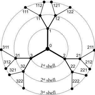
2 Technical Background 23 2.1 Husimi tree — a tool for exploring spin liquids in corner–sharing lattices 23 2.1.1 Bethe Lattice . . . . 24
2.1.2 Husimi tree . . . . 26
2.2 Monte Carlo simulations for spin systems . . . . 29
2.2.1 A fundamental sampling method . . . . 29
2.2.2 Measurement of thermodynamic observables . . . . 31 ix
x Contents
2.2.3 The Ising model . . . . 34
2.2.4 The Heisenberg model . . . . 39
2.2.5 Parallel tempering . . . . 43
2.3 Molecular dynamics . . . . 45
2.3.1 Semi–classical equations of motion . . . . 45
2.3.2 Numerical integration – 4th order Runge–Kutta . . . . 46
2.3.3 Application to spin systems . . . . 48
2.4 Correlation functions in momentum space . . . . 48
2.4.1 Dynamical structure factor . . . . 49
2.4.2 Signal sampling in time. . . . 49
2.4.3 Numerical artefacts . . . . 50
3 Curie–law crossover: thermodynamic signatures of spin liquids 53 3.1 Curie–Weiss law in conventional and unconventional magnets . . . . . 54
3.1.1 From Curie–law to Curie–Weiss law . . . . 54
3.1.2 Curie–Weiss law in spin liquids . . . . 55
3.2 Curie-law crossover . . . . 56
3.3 Validity of Husimi tree . . . . 59
3.4 Limit of Curie–Weiss fit and relevance to experiments . . . . 61
3.5 Conclusions . . . . 63
4 The Shuriken Lattice – reentrance in a novel Spin Liquid 65 4.1 The anisotropic shuriken model . . . . 66
4.2 Finite–temperature phase diagram . . . . 67
4.2.1 Long range–order: |x| >1 . . . . 67
4.2.2 Binary paramagnet: |x|< 1 . . . . 71
4.2.3 Classical spin liquid: |x| ∼ 1 . . . . 72
4.3 Reentrance of disorder . . . . 73
4.3.1 Double crossover . . . . 73
4.3.2 Correlation function in real and momentum space . . . . 75
4.3.3 Experimental realisations. . . . 78
4.4 Conclusions . . . . 79
5 Origin of spin liquid behaviour in Ca10Cr7O28 81 5.1 Synthesis of Ca10Cr7O28 . . . . 82
5.2 Thermodynamic properties in Ca10Cr7O28 . . . . 82
5.3 The bilayer breathing kagome (BBK) model . . . . 84
5.4 Magnetic excitations in Ca10Cr7O28 in theory and experiment . . . . . 86
5.4.1 Details of simulations . . . . 87
5.4.2 Polarised state at high field . . . . 87
5.4.3 Evolution of the spin–wave spectrum in field . . . . 89
5.4.4 Dynamics at zero field . . . . 89
5.5 Origin of spin liquid behaviour in the BBK model and Ca10Cr7O28 . . . 89
5.5.1 Mapping onto the J1-J2 Honeycomb model . . . . 89
5.5.2 Transverse and longitudinal excitations . . . . 94
xi 5.5.3 Band–gap opening at B = 1 T . . . . 98 5.5.4 Spin–liquid scenario in Ca10Cr7O28 . . . . 99 5.6 Conclusions . . . 100
6 Conclusions 103
A Supplementary Information for Chapter 1 107 A.1 Thermodynamics of classical oscillators . . . 107 B Supplementary Information for Chapter 2 109 B.1 Detailed balance in parallel tempering . . . 109 B.2 Linear spin–wave theory . . . 110 C Supplementary Information for Chapter 4 113 C.1 The shuriken lattice in Monte Carlo simulations . . . 113 C.2 The shuriken lattice on the Husimi tree . . . 114 C.3 The non–equilateral shuriken lattice . . . 115 D Supplementary Information for Chapter 5 117 D.1 Magnetic form factor of Cr5+ . . . 117
Bibliography 119
List of Figures
1.1 Energy spectrum of the Hubbard model for a dimer at half filling . . . 5
1.2 Landau theory for 2nd and 1st order phase transitions . . . . 10
1.3 Different frustrated unit cells. . . . 12
1.4 The kagome lattice in real materials . . . . 15
1.5 The two possible long–range ordered ground states of the classical anti- ferromagnetic Heisenberg model on the kagome lattice. . . . 17
1.6 Thermodynamics in the Heisenberg model on the kagome antiferromag- net . . . . 18
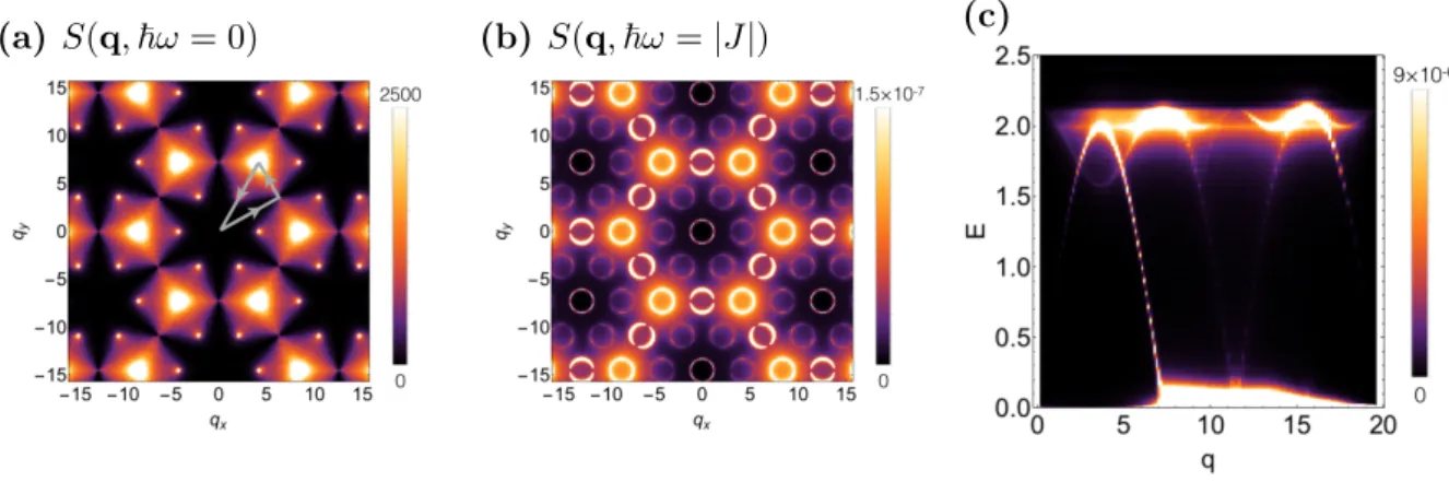
1.7 Dynamical structure factor for the Heisenberg model on the kagome antiferromagnet . . . . 19
1.8 The J1-J2-J3 Heisenberg model on the honeycomb lattice . . . . 20
2.1 Cayley tree for coordination number q = 3 up to shell n = 3 . . . . 24
2.2 The Husimi tree on the kagome lattice . . . . 27
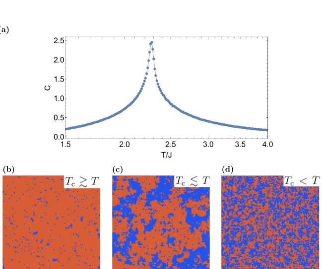
2.3 Monte Carlo simulations for the Ising model on the square lattice . . . 35
2.4 Monte Carlo scheme and simulated annealing . . . . 37
2.5 Random distributed points on a sphere . . . . 40
2.6 Uniformly distributed points on a spherical cone . . . . 41
2.7 Parallel tempering on multi–core Monte Carlo simulations . . . . 44
2.8 Sampling, following the Nyquist criterion . . . . 50
3.1 Curie–Weiss law in conventional and frustrated magnets . . . . 54
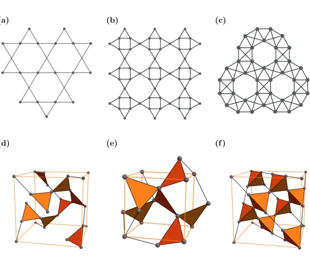
3.2 Diversity of corner sharing lattices in two and three dimensions . . . . 56
3.3 Husimi Tree on various corner sharing lattices . . . . 57
3.4 Thermodynamic properties of frustrated magnets . . . . 58
3.5 Limitations of Curie–Weiss law in spin liquids . . . . 62
4.1 The shuriken lattice with six sites per unit cell and two sublattices A and B . . . . 66
4.2 Phase diagram of the Ising model on the anisotropic shuriken lattice . . 68
4.3 Thermodynamic properties and finite–size scaling for x=−3 . . . . 69
4.4 Thermodynamic properties and finite–size scaling for x=−1.05 . . . . 70
4.5 Thermodynamic properties for different coupling ratios xshowing both, single and multiple Curie–law crossovers . . . . 74
4.6 Finite–size evolution in the double–crossover region for x= 0.9 . . . . . 75
4.7 Reduced susceptibility χT for coupling ratios x={0,±1,±0.9,±0.99}. 76 4.8 Spin–spin correlations in the vicinity of the spin liquid phases . . . . . 77
xiii
xiv List of Figures 4.9 Equal–time structure factor S(q) at zero temperature . . . . 78 5.1 Thermodynamic properties of Ca10Cr7O28 . . . . 83 5.2 Magnetic unit cell for Ca10Cr7O28and simplification to the bilayer breath-
ing kagome lattice. . . . 85 5.3 Inelastic neutron scattering data for Ca10Cr7O28 compared to theory. . 86 5.4 Spin dynamics of Ca10Cr7O28 in the saturated state at B = 11 T . . . . 88 5.5 Evolution of spin excitations as a function of magnetic field . . . . 90 5.6 Dynamical correlations in the spin–liquid phase of Ca10Cr7O28 . . . . . 91 5.7 Mapping onto an effective J1-J2 Honeycomb model . . . . 92 5.8 Phase diagram of the bilayer breathing kagome and J1-J2 Honeycomb
model . . . . 93 5.9 Evolution of the spin–wave spectrum for the bilayer breathing kagome
model in field . . . . 95 5.10 Spin dynamics in field show transverse and longitudinal excitations . . 97 5.11 Field dependency of transverse and longitudinal spin–excitations at high–
energy . . . . 98 5.12 Gap to transverse spin excitations as a function of applied magnetic field 99 C.1 The Husimi tree for the shuriken lattice . . . 114 C.2 Non–equilateral triangles in the shuriken lattice . . . 116
List of Tables
3.1 Comparison of low–temperature results from Monte Carlo simulations and Husimi tree calculations . . . . 59 4.1 Entropy S and reduced susceptibilities χT for T → 0+ with coupling
ratios |x| ≤1 . . . . 73
xv
Chapter 1
Introduction to Magnetism and Spin Liquids
“ Dass ich erkenne, was die Welt Im Innersten zusammenhält.”
Faust 1, Vers 382 f. (Faust) Johann W. v. Goethe While quantum mechanical effects on a single–particle level are well understood, magnets offer phenomena caused by collective interactions between many electrons, and provide the opportunity to unveil novel states of matter. To study the “social life”
of particles, which allows for such unconventional phases, frustrated magnets found their way into active research areas more than 30 years ago [2, 3] and grew to become one of the most active topics in many–body physics today.
Conventional magnets are described by their ordering process into a symmetry–
broken state. On the other hand, in frustrated magnets the interaction energy on all magnetic degrees of freedom cannot be minimised simultaneously, which generally suppresses conventional order. Subdominant interactions become predominant and allow for unconventional types of order and novel states of matter, like spin liquids, which do not order at any temperature.
In its own way, this research is as fundamental as the search for new particles in high–energy physics. Indeed the Higgs boson was first proposed in the context of a superconductor [4, 5, 6], while the first observation of magnetic monopoles [7, 8] and Majorana fermions [9] have taken place in magnets.
1.1 Origin of Magnetism in solids
Magnetism is one of the fundamental forces in physics, which caught the interest of researchers already in ancient times. However, a modern understanding of magnetism in solids dates back not much further than to the end of the 19th century. While e.g.
Pierre Curie[10] andPierre Weiss [11] significantly contributed to an understanding of thermodynamic properties in magnetic crystals, a microscopically exact understanding of magnetism still needed to wait until the invention of modern quantum mechanics.
1
2 Introduction to Magnetism and Spin Liquids
1.1.1 A historical summary
Magnetism has been known since antiquity from lodestone, a naturally occurring form of magnetite (Fe3O4). Greek philosophers wrote about lodestone around 800 B.C., while Chinese writings about magnetite date back to 4000 B.C., assuming that the original discoveries were made in China [12]. A pivoted–needle compass developed before 1000 A.D. has been used in China for navigation on land and water, and also became highly important in the 13th century in medieval Europe [12, 13].
However, the first scientific investigation of the phenomena of magnetism happened 1269byPierre Pélerin de Maricourt[14], who described simple laws of magnetic attrac- tion. Following de Maricourt’s work, the English scientist William Gilbert published three centuries later “De Magnete”, a landmark treatise, to be the first which clearly distinguishes electric from magnetic effects and also explains that the earth by itself behaves like a large magnet [15].
It was the danish physicistHans Christian Ørsted, who in 1819 discovered the link between electricity and magnetism, by placing a compass needle near a wire with an electric current [16]. WhileBiot,SavartandAmpereestablished the relationship of the magnetic induction and the current that generates it, James Clerk Maxwell essentially completed in 1865 the classical theory of electromagnetism by showing that electricity and magnetism represent two different aspects of the same fundamental force field [17, 18, 19]. Still without knowing the microscopic mechanism, Pierre Curie [10] and Pierre Weiss [11] contributed significantly to a modern understanding of magnetic phenomena in solid state physics by examining the effect of temperature on magnetic materials and the existence of phase transitions between magnetically ordered and disordered phases. Indeed, Pierre Curie even introduced the concept of symmetry analysis to classify ordered phases in his PhD thesis. However, a microscopically exact understanding of magnetism still needed to wait until the invention of modern quantum mechanics.
The concept of quantisation at the beginning of the 20th century introduced byMax Plank [20] and Albert Einstein [21] induced a series of discoveries in the so–called pe- riod of “old quantum theory”. Fundamental work towards a microscopic understanding of magnetism has been done by Niels Bohr [22], who quantised energy levels in the Rutherford’s atom. The famous experiment by Stern and Gerlach allowed the deter- mination of quantised angular and magnetic moments of atoms [23]. In 1921Compton suggested an intrinsic spin and therefore a magnetic moment to electrons [24], which has been proven to be correct by Goudsmit and Uhlenbeck in 1925 [25]. The magnetic moment of the electron is
ms =−gµBS
~
, (1.1)
where S is the quantised electron spin and the unit of magnetic momentum has been defined with the Bohr magneton
µB ≡ e~
2me . (1.2)
The origin of the Landé g–factor g ∼= 2.0023 could be explained by Dirac, who included relativistic aspects of electrons. With his postulation of the particle–wave
1.1 Origin of Magnetism in solids 3 duality [26], Louis de Broglie provided the starting point forSchrödinger to formulate his famous wave equation in 1926 [27]. The Schrödinger equation forms the basis of a successful description of solid–states physics and quantum statistical mechanics
HΨn =EnΨn , n ∈N, (1.3)
with the ground state Ψ0 of the system corresponding to the state with the lowest energy eigenvalue E0 of the Hamiltonian H. At the same time, Heisenberg and co–
workers developed a synonymous description of quantum systems via harmonic oscilla- tors. Hereby, the use of a coherent formulation of a non–commutative matrix algebra turns out to be a very powerful tool to assign every physical quantity a corresponding mathematical operator.
In 1933Arnold Sommerfeldintroduced the free–electron model for solids by apply- ing quantum mechanical Fermi–Dirac statistics and the Schrödinger equation to the classical Drude model [28, 29]. This concept has been formulated in second quantisa- tion as the “band theory of solids”, which averages out interaction effects by using the Hartree–Fock approximation (Stoner mean–field theory). A huge number of crystalline solids like metals and insulators could be classified using this method, but showed very quickly its limitations.
Transition and rare–earth metals have in addition to their conduction bands also partially filled d or f orbitals. It turns out, that strong Coulomb repulsion at com- mensurate filling, can suppress the electrons agility, localise them and make the ma- terial insulating, by performing a metal–insulator transition as seen for several simple transition–metal oxides [30]. Materials, which show such a behaviour are called Mott insulators [31] with many unconventional physical properties (reviewed in [32, 33]).
The magnetism within those materials cannot be explained by the band theory of solids [34, 35] and requires an extension of concepts. A microscopic model, including interactions of electrons within solids is provided by the well–known Hubbard model, which shall be described in further details in the next section.
1.1.2 Hubbard model
The unification of electricity and magnetism byMaxwell [19] and work of Pierre Curie [10] and Pierre Weiss [11] on fundamental properties of magnetic materials motivated the importance of a microscopic description of magnetism in solids. However, such a description needed to wait for a sound foundation of quantum mechanical concepts.
This was also qualitatively stated byNiels Bohrin 1911 [36] andHendrika Johanna van Leeuwenin 1921 [37], saying that magnetism in solids is a purely quantum mechanical effect and cannot be described by a classical theory (known as the Bohr–van Leeuwen theorem).
The Hubbard model was introduced in 1963 independently by Martin Gutzwiller [38],Junjiro Kanamori[39] andJohn Hubbard[40,41,42], and formulates the simplest, one–band many–body Hamiltonian which allows for a meaningful description of d and f electron systems with correlated conduction electrons.
Microscopically, those conduction electrons are allowed to occupy and hop be- tween different atomic orbitals. Spatially extended orbitals are expressed as Wannier-
4 Introduction to Magnetism and Spin Liquids functions φ(r−Ri), an orthogonal set of functions, localised around the position Ri of the ith ion and rapidly falling off to zero away from it.
In respect to the Pauli exclusion principle, electrons will be created (ˆciσ† ) and anni- hilated (ˆciσ) with spin σ at discrete pointsRi of the crystallographic lattice, following the fermionic anticommutation relations
{ˆciσ,ˆcjσ† 0}= ˆciσˆcjσ† 0 + ˆcjσ† 0ˆciσ =δi,jδσ,σ0 (1.4) {ˆciσ,ˆcjσ0}={ˆciσ† ,ˆcjσ† 0}= 0. (1.5) The Hamiltonian representing the kinetic energy of the system is
Ht =−t X
hi,jiσ
(ˆciσ†ˆcjσ+ ˆcjσ† ˆciσ), (1.6) whereas the overlap of the physical orbitals has been encoded in the hopping amplitude t. Eq. (1.6)is generally known as the tight–binding Hamiltonian [28], where delocalised electrons do not interact and lead to a conducting behaviour of the system.
Nevertheless, sufficiently dense electrons show correlation effects, due to Coulomb repulsion. A large on–site Coulomb energy
U = Z
dr1 Z
dr2 |φ(r1−Ri)|2 e2
|r1−r2| |φ(r2−Ri)|2 (1.7) restricts the hopping of electrons to already occupied orbitals and tends to form an insulator. The energy increase for doubly occupied sites is written as
HU=UX
i
nˆi↑ˆni↓ , (1.8)
where the occupation number operator is ˆniσ = ˆciσ†ˆciσ.
The Hubbard model accounts for both terms,Eq. (1.6) and Eq. (1.8) H =−t X
hi,jiσ
(ˆciσ†ˆcjσ + ˆcjσ† ˆciσ) +UX
i
ˆni↑nˆi↓ , (1.9) giving valuable insight into the nature of strongly–correlated electron systems. In the limit ofU/t1and half filling this model describes Mott insulators [43], an important group of materials in the scope of conventional and unconventional magnetism and therefore worth discussing in more detail.
1.1.3 Mott insulators
The microscopic understanding of Mott insulators does not only provide an explana- tion for the absence of electron conductivity, but also for the emergence of magnetic properties. For pedagogical reasons the magnetic properties in Mott insulators shall be demonstrated on the simple example of a half–filled dimer with strong coulomb interactions U/t1.
1.1 Origin of Magnetism in solids 5
Figure 1.1: Energy spectrum of the Hubbard model for a dimer at half filling. Exact di- agonalization of Eq. (1.10) gives a set of states, which are sepa- rated by the dominating Coulomb interaction U. A finite hopping t will split degeneracies of these states by J := 4t2/U and allows the singlet state to be the new grounds state.
The Hubbard model from Eq. (1.9) for two sites, labeled 1 and 2, reads:
Hdimer =−tX
σ
(ˆc1σ† ˆc2σ+ ˆc2σ† ˆc1σ) +U(ˆn1↑nˆ1↓+ ˆn2↑nˆ2↓), (1.10)
whereσ =↑,↓. This Hamiltonian has eigenfunctions |ψni and eigenvalues En
Hdimer|ψni=En|ψni. (1.11)
In the case of half filling (2 electrons) six possible wave functions are allowed. States with doubly occupied and one empty site form “excited” configurations, since they have to account for a large on–site Coulomb repulsion
|ex1i=| ↑↓,0i,
|ex2i=|0,↑↓i. (1.12)
Non–excited states are states with singly occupied sites. Those form one singlet and three triplet states and are denoted by their spin quantum numbers|S, Szi
|1,1i=| ↑,↑i,
|1,0i= 1
√2(| ↑,↓i+| ↓,↑i), (1.13)
|1,−1i=| ↓,↓i.
|0,0i= 1
√2(| ↑,↓i − | ↓,↑i). (1.14)
6 Introduction to Magnetism and Spin Liquids Diagonalising Eq. (1.10)reveals the following eigenvalues
E5 = 1
2(U +√
U2+ 16t2)≈U +4t2
U , (1.15)
E4 =U , (1.16)
E1 =E2 =E3 = 0, (1.17)
E0 = 1
2(U −√
U2+ 16t2)≈ −4t2
U , (1.18)
up to second order in t/U, where the energies for the triplet states are equal to zero.
The corresponding wave functions are
|ψ5i ≈ −2t
U|0,0i+ 1
√2
1− 2t2 U2
(|ex1i+|ex2i), (1.19)
|ψ4i= 1
√2(|ex1i − |ex2i), (1.20)
|ψ3i=|1,1i,
|ψ2i=|1,0i, (1.21)
|ψ1i=|1,−1i,
|ψ0i ≈
1− 2t2 U2
|0,0i+
√2t
U (|ex1i+|ex2i), (1.22) where triplet wave functions are left unchanged.
As seen inFig. 1.1the system provides degenerate states at high and low energy in absence of an electron hoppingt= 0. In a real lattice, those states would transform into bands, which then are commonly referred to as the upper and lower Hubbard bands. A finite kinetic energy t >0 splits the degeneracies by J := 4t2/U and allow the singlet
|ψ0i to be the new ground state with energy E0 <0. The ground state mixes with
|ex1i and |ex2i [Eq. (1.22)], providing a small but finite probability of finding doubly occupied sites in the ground state.
A large onsite Coulomb interactionU tseparates states of low lying energy from excited ones. It becomes quite unlikely for electrons to occupy the excited states at very low temperatures, which is why a simplification of the Hubbard model — usually achieved by a canonical transformation [43] — allows to consider just the low–lying energy states. Such a simplification leads to the celebrated Heisenberg model, the core model for most theoretical descriptions of insulating magnets.
1.1.4 Heisenberg model
The ground state properties in a Mott insulator are described by singlet and triplet states in the lower Hubbard band. Their ground state physics is well explained by the celebrated Heisenberg model:
Heff =JX
hiji
Si·Sj +const , (1.23)
1.1 Origin of Magnetism in solids 7 where P
hiji runs over all sites i connected to neighbouring sites j via the bond–
dependent exchange term Jij. The spin operator on site i is represented by the Pauli matrix σ
Si = 1 2
X
αβ
ˆciα† σαβˆciβ , (1.24) where one can see that the term Si·Sj in Eq. (1.23) accounts for virtual hopping, or also “exchange” of electrons between two connected sites.
To convince oneself, that this concept is correct, one can again consider the example of a two site Mott insulator, where the product of spin operators with eigenvalue S= 1/2is
S1·S2 = 1 2
(S1+S2)2−2S(S+ 1)
. (1.25)
It is easy to see thatS1+S2 = 0 andS1·S2 =−3/4for the singlet, whileS1+S2 = 1 andS1·S2 = 1/4for the triplet states. The result from the Hubbard model [Eq. (1.17) andEq. (1.18)] can be reproduced by takingJ = 4t2/U and the constant in Eq. (1.23) to−J/4.
Historically motivated by phenomena in Cuprate superconductors, which are basi- cally doped Mott insulators, this model has been extended to the famous t-J model [44], allowing to describe correlated systems away from half filling [43,45,46,47]. This model also allows the inclusion of higher order terms like further–neighbour interaction and higher–order spin–exchange terms, as e.g. the biquadratic term∝(S~i·S~j)2 [43].
1.1.5 Anisotropic exchange
InEq. (1.23), all spin components, Sx,Sy andSz were considered on an equal footing.
However, this is only true if effects like spin–orbit coupling are neglected. In general, the electron spin is coupled to its orbital momentum, which is influenced by the crystal field and therefore provides a mechanism where the spin can “feel” the orientation of the crystal axes. This phenomenon of magnetic anisotropy can be described by an anisotropic exchange Heisenberg Hamiltonian with the direction–dependent couplings Jz and J⊥, parallel and perpendicular to the local field axes.
H =X
hiji
Jij⊥(SixSjx+SiySjy) +JijzSizSjz
. (1.26)
In the classical limit, there are commonly three different models:
• Heisenberg model: no orientation is favoured J⊥ ≈ Jz. The spins contain O(3) symmetry, have two degrees of freedom and can point along any direction on the three–dimensional sphere.
• XY model: the crystal field suppresses the coupling between the local z–
components of the spins J⊥ Jz. The spins contain O(2) symmetry, have one degree of freedom and can point in any direction on a circle, perpendicular to the local z–direction.
8 Introduction to Magnetism and Spin Liquids
• Ising model: the crystal field favours the coupling of spins along the local z–
direction. J⊥ Jz. The spins contain Z2 symmetry and can point just in two directions.
Different lattice symmetries can produce more complicated anisotropic exchange be- haviour, such as Dzyaloshinski–Moriya interaction [48, 49].
1.2 Magnetic order in conventional magnets
Being able to formulate a microscopic model for a magnetic material is a fundamental step towards its complete physical description. However, solving such models exactly is quite often not possible, and requires approximations as given by simulation or field–
theoretical methods.
The mean–field approach is a first step to simplify a complicated model Hamil- tonian and estimate thermodynamic properties like phase transitions in conventional magnets. A general theory for explaining phase transitions and classifying various types of ordering mechanisms within them is provided by the Landau theory, which also shall be part of the discussions in this section.
1.2.1 Mean–field theory
Mean–field theory is a very general and usually the first approach to get insight into systems with complex magnetic correlations or unknown physical properties. It is an approximation, which neglects magnetic fluctuations and allows for a much simpler treatment of the problem at hand. This significant method has been introduced by Pierre Curie [10] and Pierre Weiss [11] to provide a simplified theory for phase tran- sitions in ferromagnets [50].
An illustrative example for applying mean–field theory is provided by the Ising model
H =JX
hiji
σiσj −hX
i
σi . (1.27)
Hereby, the exchange interaction J couples nearest–neighbour spins on sites i and j with Ising degree of freedom σi =±1. In the following one should considerJ <0 (fer- romagnetic interaction) on the central site σ0, which is surrounded by q neighbouring spins for the square lattice with lattice–coordination number q= 4. By averaging out fluctuations on these neighbouring spins
hσii=m 0< i≤q , (1.28) the new mean–field Hamiltonian will have the form
HM F = (J qm−h)σ0 . (1.29) The expectation value of the central site hσ0i follows from
m=hσ0i= P
{σ0}σ0 e−βHM F P
{σ0}e−βHM F
=tanh
−β(J qm−h)
, (1.30)
1.2 Magnetic order in conventional magnets 9 where translational invariance of the lattice allows to set hσii=hσ0i=m.
The self–consistent Eq. (1.30) needs to be solved numerically or graphically and provides for h = 0 one trivial (m0 = 0) and two non–trivial (m0 6= 0) solutions at exactly the critical temperature Tc
TckB
|J| =q . (1.31)
The two–dimensional square lattice with q = 4 and ferromagnetic interactions shows a phase transition temperature TckB/|J| = 4, which is comparable, but still quite different from the exact result of TckB/|J|= 2.269 [51]. Similar mean–field techniques with probably better accuracy are available by the Bethe approximation [52, 53], and models on the Bethe lattice [52,54,55], which shall be explained for frustrated lattices in more detail inSection 2.1 and Chapter 3.
However, a very general theory of phase transitions is provided by Landau theory, which shall be the topic of the next section.
1.2.2 Landau theory
Many types of phase transitions exist as e.g. melting and crystallisation, evapora- tion and condensation, but also between different forms of solids, fluid–superfluid, or conducting–superconducting transitions. It wasLev Landauin 1936 who thought about a general theory for explaining such phase transitions [56], which shall here be applied to magnets.
The standard observable representing magnetic properties is the magnetisationm, which shall in the following correspond to the magnetic order parameter of an Ising magnet. To describe the phenomenon of phase transitions Landau expanded the free energy G(m, T) close to the critical temperature Tc
∆G(m, T) =G(m, T)−G(0, T)
= b(T)
2 m2+ c(T)
4 m4+d(T)
6 m6+· · · , (1.32) here, presented for the case of the free energy function even in m. In more general models, cubic terms may also be allowed in the free energy, usually driving first order phase transitions.
It is assumed that G(m, T) is analytic at exactly the critical temperature, which generally is incorrect, since the only singular feature of a system performing a phase transition is exactly atTc. Nevertheless, Landau theory works surprisingly well in clas- sifying the nature of phase transitions and predicting physical observables in materials [57].
The temperature dependent coefficients b(T), c(T) and d(T) allow to modify the behaviour of Eq. (1.32) such that different types of magnetic phase transitions with different order can occur. The order of a phase transition equals the order of the lowest–order derivative in the free energy −∂G∂h
h=0 = m, which shows a discontinuity at the critical temperature.

![Figure 1.4: The kagome lattice in real materials, reproduced from [91].](https://thumb-ap.123doks.com/thumbv2/123deta/6958220.2273307/32.892.158.760.163.428/figure-kagome-lattice-real-materials-reproduced.webp)


![Figure 1.8: The J 1 -J 2 -J 3 Heisenberg model on the honeycomb lattice, repro- repro-duced from [120]](https://thumb-ap.123doks.com/thumbv2/123deta/6958220.2273307/37.892.108.755.164.592/figure-heisenberg-model-honeycomb-lattice-repro-repro-duced.webp)