Gerald Marchesi Dennis Pixton Lucas Sabalka
Version 1.54
A First Course in Complex Analysis
Version 1.54
Matthias Beck Gerald Marchesi
Department of Mathematics Department of Mathematical Sciences San Francisco State University Binghamton University (SUNY) San Francisco, CA 94132 Binghamton, NY 13902
[email protected] [email protected]
Dennis Pixton Lucas Sabalka
Department of Mathematical Sciences Lincoln, NE 68502 Binghamton University (SUNY) [email protected] Binghamton, NY 13902
Copyright 2002–2018 by the authors. All rights reserved. The most current version of this book is available at the website
http://math.sfsu.edu/beck/complex.html.
This book may be freely reproduced and distributed, provided that it is reproduced in its entirety from the most recent version. This book may not be altered in any way, except for changes in format required for printing or other distribution, without the permission of the authors.
The cover illustration, Square Squaredby Robert Chaffer, shows two superimposed images. The foreground image represents the result of applying a transformation,z 7→z2(see Exercises3.53 and3.54), to the background image. The locally conformable property of this mapping can be observed through matching the line segments, angles, and Sierpinski triangle features of the background image with their respective images in the foreground figure. (The foreground figure is scaled down to about 40% and repositioned to accommodate artistic and visibility considerations.) The background image fills the square with vertices at 0, 1, 1+i, and i(the positive direction along the imaginary axis is chosen as downward). It was prepared by using Michael Barnsley’s chaos game, capitalizing on the fact that a square is self tiling, and by using a fractal-coloring method. (The original art piece is in color.) A subset of the image is seen as a standard Sierpinski triangle. The chaos game was also re-purposed to create the foreground image.
Lewis Carroll (Alice in Wonderland)
About this book. A First Course in Complex Analysiswas written for a one-semester undergradu- ate course developed at Binghamton University (SUNY) and San Francisco State University, and has been adopted at several other institutions. For many of our students, Complex Analysis is their first rigorous analysis (if not mathematics) class they take, and this book reflects this very much. We tried to rely on as few concepts from real analysis as possible. In particular, series and sequences are treated from scratch, which has the consequence that power series are introduced late in the course. The goal our book works toward is the Residue Theorem, including some nontraditional applications from both continuous and discrete mathematics.
A printed paperback version of this open textbook is available from Orthogonal Publishing (www.orthogonalpublishing.com) or your favorite online bookseller.
About the authors. Matthias Beck is a professor in the Mathematics Department at San Francisco State University. His research interests are in geometric combinatorics and analytic number theory.
He is the author of three other books,Computing the Continuous Discretely: Integer-point Enumeration in Polyhedra(with Sinai Robins, Springer 2007),The Art of Proof: Basic Training for Deeper Mathematics (with Ross Geoghegan, Springer 2010), and Combinatorial Reciprocity Theorems: An Invitation to Enumerative Geometric Combinatorics(with Raman Sanyal, AMS 2018).
Gerald Marchesi is a lecturer in the Department of Mathematical Sciences at Binghamton University (SUNY).
Dennis Pixton is a professor emeritus in the Department of Mathematical Sciences at Bingham- ton University (SUNY). His research interests are in dynamical systems and formal languages.
Lucas Sabalka is an applied mathematician at a technology company in Lincoln, Nebraska.
He works on 3-dimensional computer vision applications. He was formerly a professor of mathematics at St. Louis University, after postdoctoral positions at UC Davis and Binghamton University (SUNY). His mathematical research interests are in geometric group theory, low dimensional topology, and computational algebra.
Robert Chaffer (cover art) is a professor emeritus at Central Michigan University. His academic interests are in abstract algebra, combinatorics, geometry, and computer applications. Since retirement from teaching, he has devoted much of his time to applying those interests to creation of art images (people.cst.cmich.edu/chaff1ra/Art From Mathematics).
A Note to Instructors. The material in this book should be more than enough for a typical semester-long undergraduate course in complex analysis; our experience taught us that there is more content in this book than fits into one semester. Depending on the nature of your course and its place in your department’s overall curriculum, some sections can be either partially omitted or their definitions and theorems can be assumed true without delving into proofs. Chapter10
of a course.
We would be happy to hear from anyone who has adopted our book for their course, as well as suggestions, corrections, or other comments.
Acknowledgements. We thank our students who made many suggestions for and found errors in the text. Special thanks go to Sheldon Axler, Collin Bleak, Pierre-Alexandre Bliman, Matthew Brin, Andrew Hwang, John McCleary, Sharma Pallekonda, Joshua Palmatier, and Dmytro Savchuk for comments, suggestions, and additions after teaching from this book.
We thank Lon Mitchell for his initiative and support for the print version of our book with Orthogonal Publishing, and Bob Chaffer for allowing us to feature his art on the book’s cover.
We are grateful to the American Institute of Mathematics for including our book in their Open Textbook Initiative (aimath.org/textbooks).
Contents
1 Complex Numbers 1
1.1 Definitions and Algebraic Properties . . . 2
1.2 From Algebra to Geometry and Back . . . 4
1.3 Geometric Properties . . . 8
1.4 Elementary Topology of the Plane . . . 10
Exercises . . . 13
Optional Lab . . . 18
2 Differentiation 19 2.1 Limits and Continuity . . . 19
2.2 Differentiability and Holomorphicity . . . 22
2.3 The Cauchy–Riemann Equations . . . 26
2.4 Constant Functions . . . 29
Exercises . . . 30
3 Examples of Functions 34 3.1 Möbius Transformations . . . 34
3.2 Infinity and the Cross Ratio . . . 36
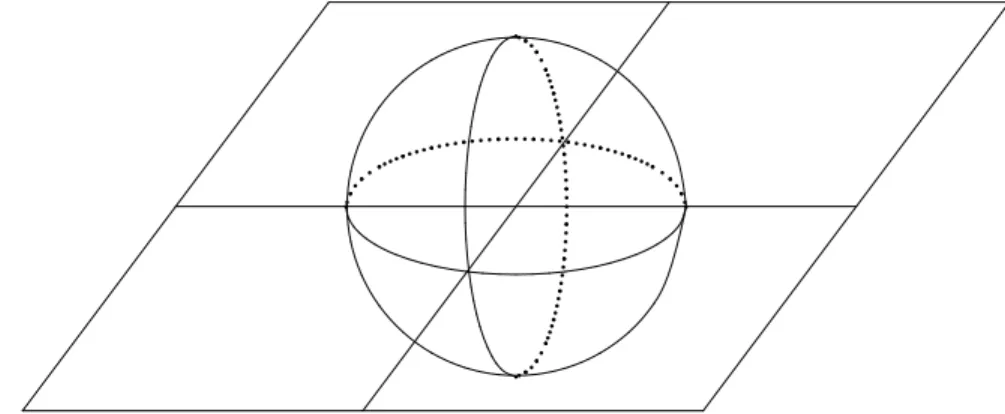
3.3 Stereographic Projection . . . 40
3.4 Exponential and Trigonometric Functions . . . 43
3.5 Logarithms and Complex Exponentials . . . 45
Exercises . . . 48
4 Integration 54 4.1 Definition and Basic Properties . . . 54
4.2 Antiderivatives . . . 58
4.3 Cauchy’s Theorem . . . 61
4.4 Cauchy’s Integral Formula. . . 65
Exercises . . . 68
5 Consequences of Cauchy’s Theorem 73 5.1 Variations of a Theme . . . 73
5.2 Antiderivatives Again . . . 76
Exercises . . . 79
6 Harmonic Functions 83 6.1 Definition and Basic Properties . . . 83
6.2 Mean-Value and Maximum/Minimum Principle . . . 86
Exercises . . . 89
7 Power Series 91 7.1 Sequences and Completeness . . . 92
7.2 Series . . . 94
7.3 Sequences and Series of Functions . . . 99
7.4 Regions of Convergence . . . 102
Exercises . . . 105
8 Taylor and Laurent Series 110 8.1 Power Series and Holomorphic Functions . . . 110
8.2 Classification of Zeros and the Identity Principle. . . 115
8.3 Laurent Series . . . 118
Exercises . . . 122
9 Isolated Singularities and the Residue Theorem 128 9.1 Classification of Singularities . . . 128
9.2 Residues . . . 133
9.3 Argument Principle and Rouché’s Theorem. . . 136
Exercises . . . 139
10 Discrete Applications of the Residue Theorem 142 10.1 Infinite Sums. . . 142
10.2 Binomial Coefficients . . . 143
10.3 Fibonacci Numbers . . . 144
10.4 The Coin-Exchange Problem . . . 144
10.5 Dedekind Sums . . . 146
Theorems From Calculus 147
Solutions to Selected Exercises 150
Index 155
Complex Numbers
Die ganzen Zahlen hat der liebe Gott geschaffen, alles andere ist Menschenwerk.
(God created the integers, everything else is made by humans.) Leopold Kronecker (1823–1891)
The real numbers have many useful properties. There are operations such as addition, subtraction, and multiplication, as well as division by any nonzero number. There are useful laws that govern these operations, such as the commutative and distributive laws. We can take limits and do calculus, differentiating and integrating functions. But you cannot take a square root of−1; that is, you cannot find a real root of the equation
x2+1=0 . (1.1)
Most of you have heard that there is a “new” numberithat is a root of (1.1); that is,i2+1= 0 ori2 =−1. We will show that when the real numbers are enlarged to a new system called the complex numbers, which includesi, not only do we gain numbers with interesting properties, but we do not lose many of the nice properties that we had before.
The complex numbers, like the real numbers, will have the operations of addition, subtraction, multiplication, as well as division by any complex number except zero. These operations will follow all the laws that we are used to, such as the commutative and distributive laws. We will also be able to take limits and do calculus. And, there will be a root of (1.1).
As a brief historical aside, complex numbers did not originate with the search for a square root of−1; rather, they were introduced in the context of cubic equations. Scipione del Ferro (1465–
1526) and Niccolò Tartaglia (1500–1557) discovered a way to find a root of any cubic polynomial, which was publicized by Gerolamo Cardano (1501–1576) and is often referred to as Cardano’s formula. For the cubic polynomial x3+px+q, Cardano’s formula involves the quantity
qq2 4 + 27p3. It is not hard to come up with examples for pandqfor which the argument of this square root becomes negative and thus not computable within the real numbers. On the other hand (e.g., by arguing through the graph of a cubic polynomial), every cubic polynomial has at least one real
1
root. This seeming contradiction can be solved using complex numbers, as was probably first exemplified by Rafael Bombelli (1526–1572).
In the next section we show exactly how the complex numbers are set up, and in the rest of this chapter we will explore the properties of the complex numbers. These properties will be of both algebraic (such as the commutative and distributive properties mentioned already) and geometric nature. You will see, for example, that multiplication can be described geometrically.
In the rest of the book, the calculus of complex numbers will be built on the properties that we develop in this chapter.
1.1 Definitions and Algebraic Properties
There are many equivalent ways to think about a complex number, each of which is useful in its own right. In this section, we begin with a formal definition of a complex number. We then interpret this formal definition in more useful and easier-to-work-with algebraic language. Later we will see several more ways of thinking about complex numbers.
Definition. Thecomplex numbersare pairs of real numbers, C := {(x,y): x,y∈R}, equipped with theaddition
(x,y) + (a,b) := (x+a, y+b) (1.2) and themultiplication
(x,y)·(a,b) := (xa−yb, xb+ya). (1.3) One reason to believe that the definitions of these binary operations are acceptable is thatCis an extension ofR, in the sense that the complex numbers of the form(x, 0)behave just like real numbers:
(x, 0) + (y, 0) = (x+y, 0) and (x, 0)·(y, 0) = (xy, 0).
So we can think of the real numbers being embedded in C as those complex numbers whose second coordinate is zero.
The following result states the algebraic structure that we established with our definitions.
Proposition 1.1. (C,+,·)is a field, that is,
for all(x,y),(a,b)∈C: (x,y) + (a,b)∈C (1.4) for all(x,y),(a,b),(c,d)∈ C: (x,y) + (a,b)+ (c,d) = (x,y) + (a,b) + (c,d) (1.5) for all(x,y),(a,b)∈C: (x,y) + (a,b) = (a,b) + (x,y) (1.6) for all(x,y)∈C: (x,y) + (0, 0) = (x,y) (1.7) for all(x,y)∈C: (x,y) + (−x,−y) = (0, 0) (1.8) for all(x,y),(a,b),(c,d)∈ C: (x,y)· (a,b) + (c,d) = (x,y)·(a,b) + (x,y)·(c,d) (1.9)
for all(x,y),(a,b)∈C: (x,y)·(a,b)∈C (1.10) for all(x,y),(a,b),(c,d)∈C: (x,y)·(a,b)·(c,d) = (x,y)· (a,b)·(c,d) (1.11) for all(x,y),(a,b)∈C: (x,y)·(a,b) = (a,b)·(x,y) (1.12) for all(x,y)∈C: (x,y)·(1, 0) = (x,y) (1.13) for all(x,y)∈C\ {(0, 0)}: (x,y)· x
x2+y2,x2−+yy2
= (1, 0) (1.14)
What we are stating here can be compressed in the language of algebra: equations (1.4)–(1.8) say that(C,+) is anAbelian groupwithidentity(0, 0); equations (1.10)–(1.14) say that(C\ {(0, 0)},·) is an Abelian group with identity(1, 0).
The proof of Proposition 1.1 is straightforward but nevertheless makes for good practice (Exercise1.14). We give one sample:
Proof of(1.8). By our definition for complex addition and properties of additive inverses inR, (x,y) + (−x,−y) = (x+ (−x), y+ (−y)) = (0, 0).
The definition of our multiplication implies the innocent looking statement
(0, 1)·(0, 1) = (−1, 0). (1.15) This identity together with the fact that
(a, 0)·(x,y) = (ax,ay)
allows an alternative notation for complex numbers. The latter implies that we can write (x,y) = (x, 0) + (0,y) = (x, 0)·(1, 0) + (y, 0)·(0, 1).
If we think—in the spirit of our remark about embeddingRinto C—of(x, 0)and(y, 0)as the real numbersxandy, then this means that we can write any complex number(x,y)as a linear combination of (1, 0) and (0, 1), with the real coefficients x and y. Now (1, 0), in turn, can be thought of as the real number 1. So if we give (0, 1) a special name, say i, then the complex number that we used to call(x,y)can be written asx·1+y·ior
x+iy.
Definition. The numberxis called thereal partandytheimaginary part1of the complex number x+iy, often denoted as Re(x+iy) =xand Im(x+iy) =y.
The identity (1.15) then reads
i2 =−1 .
In fact, much more can now be said with the introduction of the square root of −1. It is not just that (1.1) has a root, buteverynonconstant polynomial has roots inC:
1The name has historical reasons: people thought of complex numbers as unreal, imagined.
Fundamental Theorem of Algebra(see Theorem 5.11). Every nonconstant polynomial of degree d has d roots (counting multiplicity) inC.
The proof of this theorem requires some (important) machinery, so we defer its proof and an extended discussion of it to Chapter5.
We invite you to check that the definitions of our binary operations and Proposition 1.1are coherent with the usual real arithmetic rules if we think of complex numbers as given in the form x+iy.
1.2 From Algebra to Geometry and Back
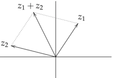
Although we just introduced a new way of writing complex numbers, let’s for a moment return to the(x,y)-notation. It suggests that we can think of a complex number as a two-dimensional real vector. When plotting these vectors in the planeR2, we will call thex-axis thereal axisand the y-axis theimaginary axis. The addition that we defined for complex numbers resembles vector addition; see Figure1.1. The analogy stops at multiplication: there is no “usual” multiplication of two vectors inR2 that gives another vector, and certainly not one that agrees with our definition of the product of two complex numbers.
DD
kk WW
z1 z2
z1+z2
Figure 1.1: Addition of complex numbers.
Any vector inR2 is defined by its two coordinates. On the other hand, it is also determined by its length and the angle it encloses with, say, the positive real axis; let’s define these concepts thoroughly.
Definition. Theabsolute value(also called themodulus) ofz=x+iyis r = |z| :=
q
x2+y2, and anargumentofz= x+iyis a numberφ∈Rsuch that
x=rcosφ and y=rsinφ.
A given complex numberz= x+iyhas infinitely many possible arguments. For instance, the number 1=1+0ilies on the positive real axis, and so has argument 0, but we could just as well say it has argument 2π, 4π,−2π, or 2πkfor any integerk. The number 0=0+0ihas modulus 0,
and every real numberφis an argument. Aside from the exceptional case of 0, for any complex numberz, the arguments of zall differ by a multiple of 2π, just as we saw for the examplez=1.
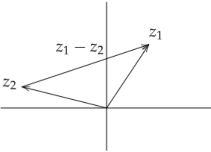
The absolute value of the difference of two vectors has a nice geometric interpretation:
Proposition 1.2. Let z1,z2 ∈ C be two complex numbers, thought of as vectors inR2, and let d(z1,z2) denote thedistancebetween (the endpoints of) the two vectors inR2(see Figure1.2). Then
d(z1,z2) = |z1−z2| = |z2−z1|.
Proof. Let z1 =x1+iy1andz2 =x2+iy2. From geometry we know that d(z1,z2) =
q
(x1−x2)2+ (y1−y2)2.
This is the definition of|z1−z2|. Since(x1−x2)2 = (x2−x1)2and (y1−y2)2 = (y2−y1)2, this is also equal to|z2−z1|.
DD
kk 44z1
z2
z1−z2
Figure 1.2: Geometry behind the distance between two complex numbers.
That |z1−z2|= |z2−z1|simply says that the vector fromz1 toz2has the same length as the vector fromz2 toz1.
It is very useful to keep this geometric interpretation in mind when thinking about the absolute value of the difference of two complex numbers.
One reason to introduce the absolute value and argument of a complex number is that they allow us to give a geometric interpretation for the multiplication of two complex numbers. Let’s say we have two complex numbers: x1+iy1, with absolute valuer1and argumentφ1, andx2+iy2, with absolute valuer2and argumentφ2. This means we can writex1+iy1= (r1cosφ1) +i(r1sinφ1) and x2+iy2 = (r2cosφ2) +i(r2sinφ2). To compute the product, we make use of some classic trigonometric identities:
(x1+iy1)(x2+iy2) = (r1cosφ1+i r1sinφ1) (r2cosφ2+i r2sinφ2)
= (r1r2cosφ1cosφ2−r1r2sinφ1sinφ2) +i(r1r2cosφ1sinφ2+r1r2sinφ1cosφ2)
= r1r2 (cosφ1cosφ2−sinφ1sinφ2) +i(cosφ1sinφ2+sinφ1cosφ2)
= r1r2 cos(φ1+φ2) +isin(φ1+φ2).
So the absolute value of the product isr1r2 and one of its arguments isφ1+φ2. Geometrically, we are multiplying the lengths of the two vectors representing our two complex numbers and adding their angles measured with respect to the positive real axis.2
FF
ff
xx
...
...
...
...
...
...
... ... . ..
... ... ... ...
...
...
...
...
...
.. ... .. ... . .. ..
.. ... .. ... ... ...
...
...
...
...
z1 z2
z1z2
φ1 φ2 φ1+φ2
Figure 1.3: Multiplication of complex numbers.
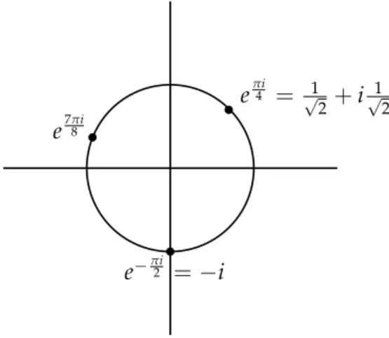
In view of the above calculation, it should come as no surprise that we will have to deal with quantities of the form cosφ+isinφ(where φis some real number) quite a bit. To save space, bytes, ink, etc., (and because “Mathematics is for lazy people”3) we introduce a shortcut notation and define
eiφ := cosφ+isinφ.
Figure 1.4 shows three examples. At this point, this exponential notation is indeed purely
e7πi8
e−πi2 =−i
eπi4 = √1
2 +i√1
2
Figure 1.4: Three sample complex numbers of the formeiφ.
a notation.4 We will later see in Chapter3 that it has an intimate connection to the complex
2You should convince yourself that there is no problem with the fact that there are many possible arguments for complex numbers, as both cosine and sine are periodic functions with period 2π.
3Peter Hilton (Invited address, Hudson River Undergraduate Mathematics Conference 2000).
4In particular, while our notation “proves”Euler’s formula e2πi=1, this simply follows from the facts sin(2π) =0
exponential function. For now, we motivate this maybe strange seeming definition by collecting some of its properties:
Proposition 1.3. For anyφ,φ1,φ2 ∈R, (a) eiφ1eiφ2 =ei(φ1+φ2)
(b) ei0 =1 (c) e1iφ =e−iφ
(d) ei(φ+2π) =eiφ (e)
eiφ =1 (f) dφd eiφ =i eiφ.
You are encouraged to prove them (Exercise 1.16); again we give a sample.
Proof of(f). By definition ofeiφ, d
dφeiφ = d
dφ(cosφ+isinφ) = −sinφ+icosφ = i(cosφ+isinφ) = i eiφ.
Proposition1.3implies that(e2πimn)n =1 for any integersmandn>0. Thus numbers of the forme2πiqwithq∈Qplay a pivotal role in solving equations of the formzn =1—plenty of reason to give them a special name.
Definition. A root of unity is a number of the form e2πimn for some integers m and n > 0.
Equivalently (by Exercise1.17), a root of unity is a complex numberζ such thatζn=1 for some positive integern. In this case, we callζ annthroot of unity. Ifnis the smallest positive integer with the propertyζn=1 thenζ is aprimitiventhroot of unity.
Example 1.4. The 4th roots of unity are±1 and±i=e±πi2. The latter two are primitive 4throots of unity.
With our new notation, the sentencethe complex number x+iy has absolute value r and argument φnow becomes the identity
x+iy = r eiφ.
The left-hand side is often called therectangular form, the right-hand side thepolar formof this complex number.
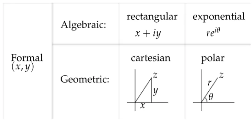
We now have five different ways of thinking about a complex number: the formal definition, in rectangular form, in polar form, and geometrically, using Cartesian coordinates or polar coordinates. Each of these five ways is useful in different situations, and translating between them is an essential ingredient in complex analysis. The five ways and their corresponding notation are listed in Figure1.5. This list is not exhaustive; see, e.g., Exercise1.21.
and cos(2π) =1. The connection between the numbersπ,i, 1, and the complex exponential function (and thus the numbere) is somewhat deeper. We’ll explore this in Section3.5.
Formal (x,y)
Algebraic:
Geometric:
rectangular exponential
cartesian polar x+iy reiθ
r x θ
y
z z
Figure 1.5: Five ways of thinking about a complex number.
1.3 Geometric Properties
From the chain of basic inequalities−px2+y2≤ −√
x2 ≤x ≤√
x2 ≤px2+y2(or, alternatively, by arguing with basic geometric properties of triangles), we obtain the inequalities
− |z| ≤ Re(z) ≤ |z| and − |z| ≤ Im(z) ≤ |z|. (1.16) The square of the absolute value has the nice property
|x+iy|2 = x2+y2 = (x+iy)(x−iy).
This is one of many reasons to give the process of passing from x+iyto x−iya special name.
Definition. The numberx−iyis the(complex) conjugateofx+iy. We denote the conjugate by x+iy := x−iy.
Geometrically, conjugatingzmeans reflecting the vector corresponding tozwith respect to the real axis. The following collects some basic properties of the conjugate.
Proposition 1.5. For any z,z1,z2∈C, (a) z1±z2= z1±z2
(b) z1·z2 =z1·z2 (c)
z1
z2
= zz1
2
(d) z =z (e) |z|=|z|
(f) |z|2 =zz
(g) Re(z) = 12(z+z) (h) Im(z) = 2i1 (z−z)
(i) eiφ =e−iφ.
The proofs of these properties are easy (Exercise 1.22); once more we give a sample.
Proof of(b). Letz1= x1+iy1andz2 =x2+iy2. Then
z1·z2 = (x1x2−y1y2) +i(x1y2+x2y1) = (x1x2−y1y2)−i(x1y2+x2y1)
= (x1−iy1)(x2−iy2) = z1·z2.
We note that(f) yields a neat formula for the inverse of a nonzero complex number, which is implicit already in (1.14):
z−1 = 1
z = z
|z|2.
A famous geometric inequality (which holds, more generally, for vectors inRn) goes as follows.
Proposition 1.6(Triangle inequality). For any z1,z2 ∈Cwe have|z1+z2| ≤ |z1|+|z2|.
By drawing a picture in the complex plane, you should be able to come up with a geometric proof of the triangle inequality. Here we proceed algebraically:
Proof. We make extensive use of Proposition 1.5:
|z1+z2|2= (z1+z2) (z1+z2) = (z1+z2) (z1+z2) = z1z1+z1z2+z2z1+z2z2
= |z1|2+z1z2+z1z2+|z2|2 = |z1|2+2 Re(z1z2) +|z2|2
≤ |z1|2+2|z1z2|+|z2|2 = |z1|2+2|z1| |z2|+|z2|2 = |z1|2+2|z1| |z2|+|z2|2
= (|z1|+|z2|)2,
where the inequality follows from (1.16). Taking square roots on the left- and right-hand side proves our claim.
For future reference we list several useful variants of the triangle inequality:
Corollary 1.7. For z1,z2, . . . ,zn ∈C, we have the following relations:
(a) The triangle inequality: |±z1±z2| ≤ |z1|+|z2|.
(b) The reverse triangle inequality: |±z1±z2| ≥|z1| − |z2|. (c) The triangle inequality for sums:
∑
n k=1zk
≤
∑
n k=1|zk|.
Inequality(a)is just a rewrite of the original triangle inequality, using the fact that|±z|=|z|, and(c)follows by induction. The proof of the reverse triangle inequality(b)is left as Exercise1.25.
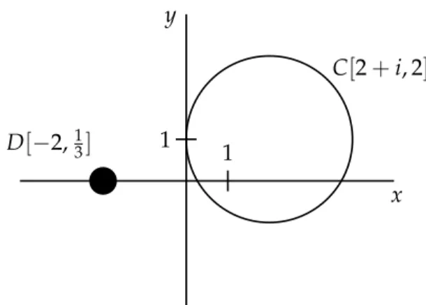
x y
C[2+i, 2] D[−2,13]
1 1
Figure 1.6: Sample circle and disk.
1.4 Elementary Topology of the Plane
In Section1.2we saw that the complex numbersC, which were initially defined algebraically, can be identified with the points in the Euclidean planeR2. In this section we collect some definitions and results concerning the topology of the plane.
In Proposition1.2, we interpreted|z−w|as the distance between the complex numbersz and w, viewed as points in the plane. So if we fix a complex number aand a positive real numberr, then allz ∈Csatisfying|z−a|=r form the set of points at distancerfroma; that is, this set is thecirclewith center aand radiusr, which we denote by
C[a,r] := {z∈C: |z−a|=r}.
The inside of this circle is called theopen diskwith centeraand radiusr; we use the notation D[a,r] := {z∈C: |z−a|<r}.
Note thatD[a,r]does not include the points onC[a,r]. Figure1.6 illustrates these definitions.
Next we need some terminology for talking about subsets ofC. Definition. SupposeGis a subset ofC.
(a) A pointa∈ Gis aninterior pointofGif some open disk with centerais a subset ofG.
(b) A pointb∈Cis aboundary pointofGif every open disk centered atbcontains a point in Gand also a point that is not inG.
(c) A pointc ∈ Cis anaccumulation point ofG if every open disk centered at ccontains a point ofGdifferent fromc.
(d) A pointd∈Gis anisolated pointofGif some open disk centered atdcontains no point of Gother than d.
The idea is that if you don’t move too far from an interior point ofGthen you remain in G;
but at a boundary point you can make an arbitrarily small move and get to a point insideGand you can also make an arbitrarily small move and get to a point outsideG.
Definition. A set isopenif all its points are interior points. A set isclosed if it contains all its boundary points.
Example 1.8. Forr >0 anda∈C, the sets{z∈C: |z−a|<r}=D[a,r]and{z∈C: |z−a|>r} are open. Theclosed disk
D[a,r] := {z∈C: |z−a| ≤r} is an example of a closed set.
A given set might be neither open nor closed. The complex planeCand theempty set∅are (the only sets that are) both open and closed.
Definition. Theboundary∂Gof a setGis the set of all boundary points ofG. Theinteriorof G is the set of all interior points ofG. TheclosureofGis the setG∪∂G.
Example 1.9. The closure of the open disk D[a,r] is D[a,r]. The boundary of D[a,r] is the circleC[a,r].
Definition. The setGisboundedifG⊆D[0,r]for somer.
One notion that is somewhat subtle in the complex domain is the idea of connectedness.
Intuitively, a set is connected if it is “in one piece.” InRa set is connected if and only if it is an interval, so there is little reason to discuss the matter. However, in the plane there is a vast variety of connected subsets.
x y
Figure 1.7: The intervals[0, 1)and(1, 2]are separated.
Definition. Two sets X,Y ⊆ C are separated if there are disjoint open sets A,B ⊂ C so that X ⊆ AandY⊆ B. A setG⊆Cisconnectedif it is impossible to find two separated nonempty sets whose union isG. Aregionis a connected open set.
The idea of separation is that the two open sets AandBensure thatXandYcannot just “stick together.” It is usually easy to check that a set isnotconnected. On the other hand, it is hard to use the above definition to show that a setisconnected, since we have to rule out any possible separation.
Example 1.10. The intervals X = [0, 1)andY = (1, 2]on the real axis are separated: There are infinitely many choices for Aand Bthat work; one choice is A=D[0, 1]andB= D[2, 1], depicted in Figure1.7. Hence X∪Y= [0, 2]\ {1}is not connected.
One type of connected set that we will use frequently is a path.
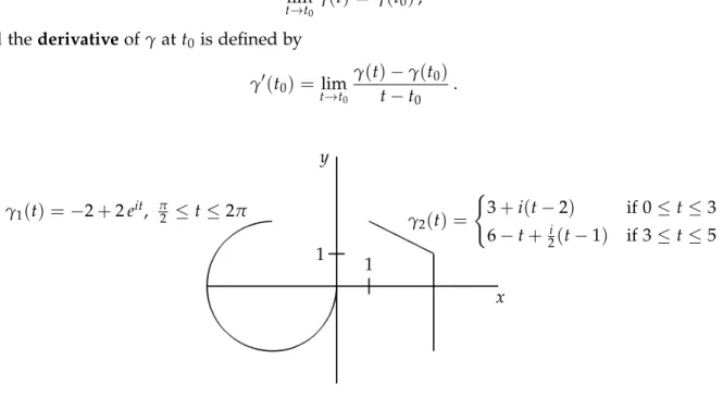
Definition. Apath(orcurve) inCis a continuous functionγ: [a,b]→C, where[a,b]is a closed interval inR. We may think ofγas a parametrization of the image that is painted by the path and will often write this parametrization asγ(t), a≤t≤ b. The path issmooth ifγis differentiable and the derivativeγ0 is continuous and nonzero.5
This definition uses the calculus notions of continuity and differentiability; that is,γ: [a,b]→C beingcontinuousmeans that for all t0 ∈[a,b]
tlim→t0
γ(t) =γ(t0), and thederivativeofγatt0 is defined by
γ0(t0) = lim
t→t0
γ(t)−γ(t0) t−t0 .
x y
1 1 γ1(t) =−2+2eit, π2 ≤t≤2π
γ2(t) =
(3+i(t−2) if 0≤t≤3 6−t+ 2i(t−1) if 3≤t≤5
Figure 1.8: Two paths and their parametrizations;γ1is smooth andγ2is continuous and piecewise smooth.
Figure1.8shows two examples. We remark that each path comes with anorientation, i.e., a sense of direction. For example, the pathγ1 in Figure1.8is different from
γ3(t) =−2+2e−it, 0≤t ≤ 3π2 ,
5There is a subtlety here, becauseγis defined on a closed interval. Forγ:[a,b]→Cto be smooth, we demand both thatγ0(t)exists for alla<t<b, and that limt→a+γ0(t)and limt→b−γ0(t)exist.
even though bothγ1andγ3yield the same picture: γ1 features a counter-clockwise orientation, where as that of γ3is clockwise.
It is a customary and practical abuse of notation to use the same letter for the path and its parametrization. We emphasize that a path must have a parametrization, and that the parametrization must be defined and continuous on a closed and bounded interval[a,b]. Since topologically we may identify C with R2, a path can be specified by giving two continuous real-valued functions of a real variable,x(t)andy(t), and settingγ(t) =x(t) +i y(t).
Definition. The path γ: [a,b] → Cissimple if γ(t)is one-to-one, with the possible exception thatγ(a) =γ(b)(in plain English: the path does not cross itself). A pathγ:[a,b]→Cisclosed ifγ(a) =γ(b).
Example 1.11. Theunit circle C[0, 1], parametrized, e.g., byγ(t) = eit, 0 ≤ t ≤ 2π, is a simple closed path.
As seems intuitively clear, any path is connected; however, a proof of this fact requires a bit more preparation in topology. The same goes for the following result, which gives a useful property of open connected sets.
Theorem 1.12. If any two points in G ⊆ C can be connected by a path in G, then G is connected.
Conversely, if G⊆Cis open and connected, then any two points of G can be connected by a path in G; in fact, we can connect any two points of G by a chain of horizontal and vertical segments lying in G.
Here achain of segmentsin Gmeans the following: there are pointsz0,z1, . . . ,zn so thatzk andzk+1 are the endpoints of a horizontal or vertical segment inG, for allk =0, 1, . . . ,n−1. (It is not hard to parametrize such a chain, so it determines a path.)
Example 1.13. Consider the openunit diskD[0, 1]. Any two points inD[0, 1]can be connected by a chain of at most two segments inD[0, 1], and soD[0, 1]is connected. Now let G=D[0, 1]\ {0}; this is the punctured disk obtained by removing the center fromD[0, 1]. ThenGis open and it is connected, but now you may need more than two segments to connect points. For example, you need three segments to connect−12 to 12 since we cannot go through 0.
We remark that the second part of Theorem 1.12is not generally true if Gis not open. For example, circles are connected but there is no way to connect two distinct points of a circle by a chain of segments that are subsets of the circle. A more extreme example, discussed in topology texts, is the “topologist’s sine curve,” which is a connected setS ⊂ Cthat contains points that cannot be connected by a path of any sort withinS.
Exercises
1.1.Let z=1+2iandw=2−i. Compute the following:
(a) z+3w (b) w−z
(c) z3
(d) Re(w2+w)
(e) z2+z+i
1.2.Find the real and imaginary parts of each of the following:
(a) zz−+aa for any a∈R (b) 37i++5i1
(c)
−1+i√ 3 2
3
(d) infor any n∈Z
1.3.Find the absolute value and conjugate of each of the following:
(a) −2+i
(b) (2+i)(4+3i)
(c) √3−i
2+3i (d) (1+i)6
1.4.Write in polar form:
(a) 2i (b) 1+i
(c) −3+√ 3i
(d) −i (e) (2−i)2
(f) |3−4i|
(g) √ 5−i
(h)
1√−i 3
4
1.5.Write in rectangular form:
(a) √ 2ei3π4 (b) 34eiπ2
(c) −ei250π (d) 2e4πi 1.6.Write in both polar and rectangular form:
(a) eln(5)i (b) dφd eφ+iφ
1.7.Show that the quadratic formula works. That is, fora,b,c∈Rwitha6=0, prove that the roots of the equationaz2+bz+c=0 are
−b±√
b2−4ac
2a .
Here we define√
b2−4ac =i√
−b2+4acif thediscriminantb2−4acis negative.
1.8.Use the quadratic formula to solve the following equations.
(a) z2+25=0 (b) 2z2+2z+5=0
(c) 5z2+4z+1=0 (d) z2−z=1
(e) z2=2z
1.9.Find all solutions of the equationz2+2z+ (1−i) =0.
1.10.Fixa∈Candb∈ R. Show that the equation|z2|+Re(az) +b=0 has a solution if and only if|a2| ≥4b. When solutions exist, show the solution set is a circle.
1.11.Find all solutions to the following equations:
(a) z6=1 (b) z4=−16
(c) z6=−9 (d) z6−z3−2=0 1.12.Show that|z|=1 if and only if 1z =z.
1.13.Show that
(a) zis a real number if and only ifz =z;
(b) zis either real or purely imaginary if and only if(z)2=z2. 1.14.Prove Proposition1.1.
1.15.Show that ifz1z2=0 thenz1=0 orz2=0.
1.16.Prove Proposition1.3.
1.17.Fix a positive integern. Prove that the solutions to the equationzn=1 are preciselyz= e2πimn wherem∈Z. (Hint: To show that every solution ofzn=1 is of this form, first prove that it must be of the formz =e2πian for somea ∈R, then write a=m+bfor some integermand some real number 0≤b<1, and then argue thatbhas to be zero.)
1.18.Show that
z5−1 = (z−1) z2+2zcosπ5 +1
z2−2zcos2π5 +1 and deduce from this closed formulas for cosπ5 and cos2π5 .
1.19.Fix a positive integernand a complex numberw. Find all solutions tozn=w. (Hint: Write win terms of polar coordinates.)
1.20.Use Proposition1.3to derive the triple angle formulas:
(a) cos(3φ) =cos3φ−3 cosφsin2φ (b) sin(3φ) =3 cos2φsinφ−sin3φ
1.21.Givenx,y∈R, define the matrix M(x,y):=
x −y
y x
. Show that
M(x,y) +M(a,b) = M(x+a,y+b) and M(x,y)M(a,b) = M(xa−yb, xb+ya). (This means that the set{M(x,y): x,y∈R}, equipped with the usual addition and multiplication of matrices, behaves exactly likeC={(x,y): x,y∈R}.)
1.22.Prove Proposition1.5.
1.23.Sketch the following sets in the complex plane:
(a) {z∈C: |z−1+i|=2} (b) {z∈C: |z−1+i| ≤2}
(c) {z∈C: Re(z+2−2i) =3} (d) {z∈C: |z−i|+|z+i|=3}
(e) {z∈C: |z|=|z+1|}
(f) {z∈C: |z−1|=2|z+1|}
(g)
z∈C: Re(z2) =1 (h)
z∈C: Im(z2) =1 1.24.Supposep is a polynomial with real coefficients. Prove that
(a) p(z) = p(z).
(b) p(z) =0 if and only ifp(z) =0.
1.25.Prove the reverse triangle inequality (Proposition1.7(b)) |z1−z2| ≥ |z1| − |z2|. 1.26.Use the previous exercise to show that
1 z2−1
≤ 1 3 for everyz on the circleC[0, 2].
1.27.Sketch the sets defined by the following constraints and determine whether they are open, closed, or neither; bounded; connected.
(a) |z+3|<2 (b) |Im(z)|<1
(c) 0<|z−1|<2
(d) |z−1|+|z+1|=2 (e) |z−1|+|z+1|<3
(f) |z| ≥Re(z) +1 1.28.What are the boundaries of the sets in the previous exercise?
1.29.LetGbe the set of points z∈ Csatisfying either zis real and −2 < z< −1, or|z|< 1, or z=1 or z=2.
(a) Sketch the setG, being careful to indicate exactly the points that are inG.
(b) Determine the interior points ofG.
(c) Determine the boundary points ofG.
(d) Determine the isolated points ofG.
1.30.The setGin the previous exercise can be written in three different ways as the union of two disjoint nonempty separated subsets. Describe them, and in each case say briefly why the subsets are separated.
1.31.Show that the union of two regions with nonempty intersection is itself a region.
1.32.Show that if A⊆Band Bis closed, then ∂A⊆B. Similarly, if A⊆B and Ais open, show that Ais contained in the interior of B.
1.33.Find a parametrization for each of the following paths:
(a) the circleC[1+i, 1], oriented counter-clockwise (b) the line segment from−1−ito 2i
(c) the top half of the circleC[0, 34], oriented clockwise
(d) the rectangle with vertices±1±2i, oriented counter-clockwise (e) the ellipse{z∈C: |z−1|+|z+1|=4}, oriented counter-clockwise 1.34.Draw the path parametrized by
γ(t) =cos(t)|cos(t)|+isin(t)|sin(t)|, 0≤ t≤2π.
1.35.LetGbe the annulus determined by the inequalities 2<|z|<3. This is a connected open set. Find the maximum number of horizontal and vertical segments inGneeded to connect two points ofG.
Optional Lab
Open your favorite web browser and search for thecomplex function grapherfor the open-source softwaregeogebra.
1. Convert the following complex numbers into their polar representation, i.e., give the absolute value and the argument of the number.
34= i= −π = 2+2i= −1
2 √
3+i
=
Afteryou have finished computing these numbers, check your answers with the program.
2. Convert the following complex numbers given in polar representation into their rectangular representation.
2ei0 = 3eπi2 = 12eiπ = e−3πi2 = 2e3πi2 =
Afteryou have finished computing these numbers, check your answers with the program.
3. Pick your favorite five numbers from the ones that you’ve played around with and put them in the tables below, in both rectangular and polar form. Apply the functions listed to your numbers. Think about which representation is more helpful in each instance.
rectangular polar z+1 z+2−i
2z
−z
z 2
iz z z2 Re(z) Im(z) iIm(z)
|z|
1 z
4. Play with other examples until you get a feel for these functions.
Differentiation
Mathematical study and research are very suggestive of mountaineering. Whymper made several efforts before he climbed the Matterhorn in the 1860’s and even then it cost the life of four of his party. Now, however, any tourist can be hauled up for a small cost, and perhaps does not appreciate the difficulty of the original ascent. So in mathematics, it may be found hard to realise the great initial difficulty of making a little step which now seems so natural and obvious, and it may not be surprising if such a step has been found and lost again.
Louis Joel Mordell (1888–1972)
We will now start our study of complex functions. The fundamental concept on which all of calculus is based is that of a limit—it allows us to develop the central properties of continuity and differentiability of functions. Our goal in this chapter is to do the same for complex functions.
2.1 Limits and Continuity
Definition. A(complex) function f is a map from a subsetG⊆CtoC; in this situation we will write f :G→Cand callGthedomainof f. This means that each elementz∈Ggets mapped to exactly one complex number, called theimageofz and usually denoted by f(z).
So far there is nothing that makes complex functions any more special than, say, functions from Rm to Rn. In fact, we can construct many familiar looking functions from the standard calculus repertoire, such as f(z) = z (theidentity map), f(z) = 2z+i, f(z) = z3, or f(z) = 1z. The former three could be defined on all ofC, whereas for the latter we have to exclude the origin z=0 from the domain. On the other hand, we could construct some functions that make use of a certain representation ofz, for example, f(x,y) =x−2iy, f(x,y) =y2−ix, or f(r,φ) =2r ei(φ+π).
Next we define limits of a function. The philosophy of the following definition is not restricted to complex functions, but for sake of simplicity we state it only for those functions.
Definition. Suppose f :G→Candz0is an accumulation point ofG. Ifw0is a complex number such that for everye>0 we can findδ >0 so that, for allz∈ Gsatisfying 0<|z−z0|< δ, we
19
have|f(z)−w0|<e, thenw0 is thelimitof f aszapproachesz0; in short,
zlim→z0
f(z) = w0.
This definition is the same as is found in most calculus texts. The reason we require thatz0is an accumulation point of the domain is just that we need to be sure that there are pointszof the domain that are arbitrarily close toz0. Just as in the real case, our definition (i.e., the part that says 0 <|z−z0|) does not require that z0is in the domain of f and, ifz0is in the domain of f, the definition explicitly ignores the value of f(z0).
Example 2.1. Let’s prove that lim
z→iz2 =−1.
Givene>0, we need to determineδ>0 such that 0<|z−i|< δimplies|z2+1|< e. We rewrite
z2+1
= |z−i| |z+i| < δ|z+i|.
If we chooseδ, say, smaller than 1 then the factor|z+i|on the right can be bounded by 3 (draw a picture!). This means that anyδ <min{e3, 1}should do the trick: in this case, 0< |z−i|<δ implies
z2+1
< 3δ < e.
This was a proof written out in a way one might come up with it. Here’s a short, neat version:
Given e>0, choose 0<δ <min{3e, 1}. Then 0<|z−i|< δimplies
|z+i| = |z−i+2i| ≤ |z−i|+|2i| < 3 , so
z2−(−1) = z2+1
= |z−i| |z+i| < 3δ < e. This proves limz→iz2 =−1.
Just as in the real case, the limit w0 is unique if it exists (Exercise2.3). It is often useful to investigate limits by restricting the way the pointzapproachesz0. The following result is a direct consequence of the definition.
Proposition 2.2. Suppose f : G→ Candlimz→z0 f(z) =w0. SupposeGe ⊆ G and z0is an accumula- tion point ofG. Ife ef is the restriction of f toG thene limz→z0 ef(z)exists and has the value w0.
The definition oflimitin the complex domain has to be treated with a little more care than its real companion; this is illustrated by the following example.
Example 2.3. The limit of zz asz →0 does not exist.
To see this, we try to compute this limit as z→0 on the real and on the imaginary axis. In the first case, we can writez=x ∈R, and hence
limz→0
z
z = lim
x→0
x
x = lim
x→0
x x = 1 . In the second case, we writez=iy wherey∈R, and then
limz→0
z
z = lim
y→0
iy
iy = lim
y→0
−iy
iy = −1 .
So we get a different “limit” depending on the direction from which we approach 0. Proposition2.2 then implies that the limit of zz asz→0 does not exist.
On the other hand, the following usual limit rules are valid for complex functions; the proofs of these rules are everything but trivial and make for nice practice (Exercise2.4); as usual, we give a sample proof.
Proposition 2.4. Let f and g be complex functions with domain G, let z0be an accumulation point of G, and let c∈C. Iflimz→z0 f(z)andlimz→z0 g(z)exist, then
(a) lim
z→z0
(f(z) +c g(z)) = lim
z→z0
f(z) +c lim
z→z0
g(z) (b) lim
z→z0
(f(z)·g(z)) = lim
z→z0
f(z)· lim
z→z0
g(z) (c) lim
z→z0
f(z)
g(z) = limz→z0 f(z) limz→z0g(z)
where in the last identity we also require thatlimz→z0g(z)6=0.
Proof of(a). Assume thatc6=0 (otherwise there is nothing to prove), and letL=limz→z0 f(z)and M=limz→z0 g(z). Then we know that, givene>0, we can findδ1,δ2>0 such that
0<|z−z0|<δ1 implies |f(z)−L|< e 2 and
0<|z−z0|<δ2 implies |g(z)−M|< e 2|c|. Thus, choosing δ=min{δ1,δ2}, we infer that 0<|z−z0|<δ implies
|(f(z) +c g(z))−(L+c M)| ≤ |f(z)−L|+|c| |g(z)−M| < e.
Here we used the triangle inequality (Proposition1.6). This proves that limz→z0(f(z) +c g(z)) = L+c M, which was our claim.
Because the definition of the limit is somewhat elaborate, the following fundamental definition looks almost trivial.
Definition. Suppose f : G→C. Ifz0∈ Gand eitherz0 is an isolated point ofGor
zlim→z0 f(z) = f(z0)
then f iscontinuousatz0. More generally, f iscontinuousonE⊆ Gif f is continuous at every z∈ E.
However, in almost all proofs using continuity it is necessary to interpret this in terms of e’s andδ’s. So here is an alternate definition:
Definition. Suppose f :G→Candz0∈ G. Then f iscontinuousatz0if, for every positive real numberethere is a positive real numberδso that
|f(z)− f(z0)|<e for all z∈ G satisfying |z−z0|< δ.
See Exercise2.11for a proof that these definitions are equivalent.
Example 2.5. We already proved (in Example2.1) that the function f :C→Cgiven by f(z) =z2 is continuous atz=i. You’re invited (Exercise2.8) to extend our proof to show that, in fact, this function is continuous onC.
On the other hand, let g:C→Cbe given by g(z):=
(z
z ifz6=0 , 1 ifz=0 .
In Example 2.3we proved that g is not continuous atz = 0. However, this is its only point of discontinuity (Exercise2.9).
Just as in the real case, we can “take the limit inside” a continuous function, by considering composition of functions.
Definition. Theimage of the function g : G → Cis the set {g(z): z ∈G}. If the image ofg is contained in the domain of another function f :H→C, we define thecomposition f ◦g:G→C through
(f◦g)(z) := f(g(z)).
Proposition 2.6. Let g : G → C with image contained in H, and let f : H → C. Suppose z0 is an accumulation point of G, limz→z0 g(z) = w0 ∈ H, and f is continuous at w0. Thenlimz→z0 f(g(z)) =
f(w0); in short,
zlim→z0 f(g(z)) = f
zlim→z0g(z)
. Proof. Given e>0, we know there is anη>0 such that
|w−w0|< η implies |f(w)− f(w0)|<e. For thisη, we also know there is aδ>0 such that
0< |z−z0|< δ implies |g(z)−w0|< η. Stringing these two implications together gives that
0<|z−z0|<δ implies |f(g(z))− f(w0)|< e. We have thus proved that limz→z0 f(g(z)) = f(w0).
2.2 Differentiability and Holomorphicity
The fact that simple functions such as zz do not have limits at certain points illustrates something special about complex numbers that has no parallel in the reals—we can express a function in a very compact way in one variable, yet it shows some peculiar behavior in the limit. We will repeatedly notice this kind of behavior; one reason is that when trying to compute a limit of
![Figure 1.7: The intervals [ 0, 1 ) and ( 1, 2 ] are separated.](https://thumb-ap.123doks.com/thumbv2/123deta/7004890.2288779/17.918.312.613.727.928/figure-intervals-separated.webp)