Studies On Different Solution Pattern Of Linear And Quadratic Algebraic Equation: A Variant Of Newton’s Method

Studies On Different Solution Pattern Of Linear And Quadratic Algebraic Equation: A Variant Of Newton’s Method

*Dr. Rajeev Kumar and **Geeta Arora

*Assistant Professor, Department of Mathematics, OPJS University, Churu, Rajasthan (India)

**Research Scholar, Department of Mathematics, OPJS University, Churu, Rajasthan (India) Email: [email protected]; Contact No. +91-9518073997

Abstract: It is found that not only the model (equation (1.5)) and its derivative agree with the function f ( x )

and its derivative f ' ( x ),

respectively, but the second derivative of the model and the second derivative of the function are also agreeing at the current iterate x  x

ⁿ

(Fernando and Weerakoon [1997]). Even though the model for Newton’s method matches with the values of the slope f ' ( x

_n

)

of the function, it does not match with its curvature in terms of

) ( '' x

_n

f . It was found that the computational order of convergence is more than three in some cases in variant of Newton’s method, which is higher than the classical Newton’s method. The number of function evaluations was found to be less for variant of Newton’s method as compared to classical Newton’s method. Another important characteristic of this method is that it does not require second or higher derivatives of the function to carry out iterations.

[Kumar, R. and Arora, G. Studies On Different Solution Pattern Of Linear And Quadratic Algebraic Equation:

A Variant Of Newton’s Method. Academ Arena 2020;12(2):9-13]. ISSN 1553-992X (print); ISSN 2158-771X (online). http://www.sciencepub.net/academia. 2. doi:10.7537/marsaaj120220.02.

Keywords: Solution, Linear, Quadratic, Newton Method

1.1 Introduction

In this study, authors have suggested an improvement over the Newton’s method at the expense of one additional first derivative evaluation. Derivation of Newton’s method involves an indefinite integral of the derivative of the function, and the relevant area is approximated by a rectangle. Here authors have approximated this indefinite integral by a trapezoid instead of a rectangle, and the resulted method has third-order convergence, i.e., the method approximately triples the number of significant digits after some iterations. Computed results overwhelmingly support this theory, and

computational order of convergence was even more then three for certain functions. It is important to understand how Newton’s method is constructed. At each iterative step construct a local model of the function f (x )

at the point x

ⁿ

and solve for the root x

^n1

of the local model. In Newton’s method, shown in figure 1.1, the local linear model is the tangent drawn to the function f ( x )

at the contact point x

ⁿ

as:

).

( ) ( ' ) ( )

(

_{n n n}

n

x f x f x x x

M    _…(1.1)

Dennis [1983] interpreted local linear model in another way. From Newton’s theorem,

 

 ^x

n x

n

d f x

f x

f ( ) ( ) ' (  )  .

…(1.2)

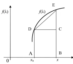
Dennis [1983] replaced the indefinite integral by the rectangle ABCD as shown in figure 1.2, i.e.,

), (

) ( ' )

(

'

_n

x

x

f d f x

n

x x

n



 ^{ }  _…(1.3)

which results in the model given in equation (1.1). In this the area DCE is ignored.

1.2 A Variant of Newton’s Method

In this paper the authors have approximated the indefinite integral involved in equation (1.2) by the trapezium ABED as shown in figure 1.3, i.e.,

 ' ( ) ' ( )  . )

2 ( ) 1

(

' d x x f x f x

f

_{n n}

x

x_n

  



 



 

 ^{ }

…(1.4) Thus, the local modal is given by

Figure 1.1: Newton’s iterative step.

Figure 1.2: Approximating the area by the rectangle ABCD.



 ( ) )

(

_n

n

x f x

M

 ' ( ) ' ( )  . )

2 (

1  x  x

_n

f x

_n

 f x



 





…(1.5)

It is found that not only the model (equation (1.5)) and its derivative agree with the function f ( x )

and its derivative f ' ( x ),

respectively, but the second derivative of the model and the second derivative of the function are also agreeing at the current iterate

x

n

x 

(Fernando and Weerakoon [1997]). Even though the model for Newton’s method matches with the values of the slope f ' ( x

_n

)

of the function, it does not match with its curvature in terms of f '' ( x

_n

)

.

Figure 1.3: Approximating the area by the trapezoid ABCD.

The next iterative point as the root of the local model (equation (1.5)) is

, 0 ) (

_n1



n

x

M

 ' ( ) ' ( )  0 )

1 ( )

(     

 

 x x f x f x

x f

f(λ) f(λ)

A ^B

C D

E

x x

n

0

f(λ) f(λ)

A ^B

C D

E

x x

_n

0



) . ( ' ) ( '

) ( 2

1 1





  

n n

n n

n

f x f x

x x f

x

…(1.6) This is an implicit scheme, which means

derivative of the function at the

n 1 )

th

( 

iterative step is used to calculate the

n 1 )

th

( 

iterate. This difficulty is overcome by using Newton’s method to

compute the

n 1 )

th

( 

iterate on the right-hand side.

Therefore, the resulting scheme is

 ^{' ( ) ' ( )}  ^{, 0 , 1 , 2 ,...}

) ( 2

* 1

1



 







n

x f x f

x x f

x

n n

n n

n

…(1.7)

where

) . ( '

)

*

(

1

n n n

n

f x

x x f

x

_

 

…(1.8)

1.3 Convergence of Method

Let  be a simple root of f ( x )

, i.e., f (  )  0

and f ' (  )  0

. Let approximate value of the root is given by x

ⁿ

   e

ⁿ

, where e

n

is the error. Using Taylor expansion f ( x

_n

)

can be written as:

) (

)

( x

_n

f e

_n

f   

) ( )

! ( 3 ) 1

! ( 2 ) 1 ( )

( f

⁽¹⁾

e

_n

f

⁽²⁾

e

_n²

f

⁽³⁾

e

_n³

O e

_n⁴

f    

    

 



 

   

 ( )

) (

) (

! 3

1 ) (

) (

! 2 ) 1

(

₍₁₎ ⁴

3 ) 3 (

) 1 (

2 ) 2 ( )

1 (

n n

n

n

O e

f

e f

f

e e f

f 





 

 ^{( )}  ^,

)

(

₂ ² ₃ ^{3 4}

) 1 (

n n

n

n

C e C e O e

e

f   

  _…(1.9)

where C

_j

 ( 1 / j ! ) f

^(j)

(  ) / f

⁽¹⁾

(  ).

Similarly, using Taylor expansion,

) (

) (

⁽¹⁾

) 1 (

n

n

f e

x

f   

 ^{1 2 3 ( )}  ^.

)

(

_{2 3} ^{2 3}

) 1 (

n n

n

C e O e

e C

f   

  _…(1.10)

Dividing equation (1.9) by equation (1.10) and after some simplifications, one gets,

) (

) (

) 1 (

n n

x f

x f

), ( )

2 2

(

₂² ₃ ^{3 4}

2

2 n n n

n

C e C C e O e

e    

 _…(1.11)

Substituting the results from equation (1.11) in equation (1.8), one gets,

* 1



x n    C

₂

e

_n²

 ( 2 C

₃

 2 C

₂²

) e

³_n

 O ( e

_n⁴

).

…(1.12)

This value of

* 1



x n

is used for the Taylor’s series expansion of  ^* 1 

) 1 (



x n

f as,

] ) ( ) ( ) ( )

2 2

( [

) ( )

(

^*₁ ⁽¹⁾ ₂ ² _{3 2}^{2 3 4 (2) 4}

) 1 (

n n

n n

n

f C e C C e O e f O e

x

f

_

       

 1 2 4 ( ) ( )  .

)

(

₂^{2 2} _{2 3 2}^{2 3 4}

) 1 (

n n

n

C C C e O e

e C

f    

  _…(1.13)

Adding equation (1.10) and equation (1.13),

 



 

  



 



 









_

( )

2 1 3

) ( 2 ) ( )

(

^{(1) *} ₁ ⁽¹⁾ _{2 2}² ₃ ^{2 3}

) 1 (

n n

n n

n

f x f C e C C e O e

x

f 

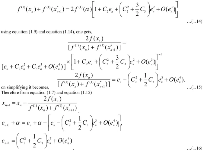
…(1.14) using equation (1.9) and equation (1.14), one gets,

 (

^_

) ]  )

( [

) ( 2

1 ) 1 ( )

1 (

n n

n

x f x f

x f

] ) ( [ e

_n

 C

₂

e

_n²

 C

₃

e

_n³

 O e

_n⁴

1 3 2

3 2

2

2

( )

2 1 3



 



 

  



 



 





 C e

_n

C C e

_n

O e

_n

on simplifying it becomes, [ ( ) ( ) ] )

( 2

* 1 ) 1 ( )

1 (



_n n

n

x f x f

x

f ( ).

2

1

_{3 4}

3 2

2 n n

n

C C e O e

e  



 



 





…(1.15) Therefore from equation (1.7) and equation (1.15)

) ( )

(

) ( 2

* 1 ) 1 ( )

1 1 (





  

n n

n n

n

f x f x

x x f

x

,

, ) 2 (

1

_{3 4}

3 2

2

1







 

  



 



 













n n n n

n

e e C C e O e

e  

) 2 (

1

_{3 4}

3 2

2

1 n n

n

C C e O e

e  



 



 





. …(1.16)

This shows that the proposed method has third-order convergence.

Table 1.1: Examples used for comparison of Varient’s Newton method and classical Newton’s method

S.No. Functions Root

1. x

³

 4 x

²

 10  0 1.36523001341448

1. sin ² x  x ²  1  0 1.40449164821621

3. x

²

 e

^x

 3 x  2  0 0.25753028543977

4. cos x  x  0 0.73908513321475

5. ( x  1 )

³

 1  0 1.00000000000000

6. x

³

 10  0 1.15443469003367

7. xe

^x2

 sin

²

x  3 cos x  5  0  1 . 20764782713013

8. x

²

sin

²

x  e

^x2cosxsinx

 28  0 4.82458931731526

9. e

^x27x30

 1  0 3.00000000000000

1.4 Numerical Examples

The authors have demonstrated the use of their variant of Newton’s method over the classical Newton’s method for the examples given in Table 1.1.

The roots were found correct to 15 decimal places.

From Table 1.1 it was found that the

computational order of convergence is more than three

in some cases in variant of Newton’s method, which is

higher than the classical Newton’s method. The

number of function evaluations was found to be less for

this method is that it does not require second or higher derivatives of the function to carry out iterations.

Corresponding author:

Mrs. Geeta Arora

Research Scholar, Department of Mathematics, OPJS University, Churu,

Rajasthan (India)

Contact No. +91-9518073997 Email- [email protected] References:

1. Cooley L., Trigueros M., Baker B. Schema thematization: A framework and an example.

Journal for Research in Mathematics Education.

2007; 38: 370-392.

2. Corbin, L., & Strauss, A. (2008). Basics of qualitative research. Techniques and procedures for developing grounded theory. Los Angeles:

Sage.

3. Czarnocha B., Dubinsky E., Prabhu V., Vidakovic D. One theoretical perspective in undergraduate mathematics education research.

In: O. Zaslavsky, editor. Proceedings of the 23rd Conference of PME. Haifa, Israel: PME. 1999; 1:

95–110.

4. D. Chen, On the convergence of a class of generalized Steffensen’s iterative procedures and error analysis. Int. J. Comput. Math., 31 (1989), 195–203.

5. D. E. Goldberg, Genetic Algorithms in Search, Optimization and Machine Learning. Reading, MA: Addison-Wesley, 1989.

6. D. Kincaid and W. Cheney, Numerical Analysis, second ed., Brooks/Cole, Pacific Grove, CA (1996).

7. Davis, R. B. (1992). Understanding

“understanding”. Journal of Mathematical Behavior, 11, 225−241.

8. Dennis J.E. and Schnable R.B., Numerical Methods for Unconstrained Optimisation and Nonlinear Equations, Prentice Hall, 1983.

9. Department of Education, Training and Employment. (2013). Curriculum into the classroom (C2C). Retrieved from education.qld.gov.au/c2c

10. Dheghain, M. and Hajarian, M. 2010. New iterative method for solving nonlinear equations fourth-order Convergence. International Journal of Computer Mathematics 87: 834- 839.

11. Didis M. G., Baş S., Erbaş A. K. Students’

reasoning in quadratic equations with one unknown. Paper presented at the 7th Congress of the European Society for Research in Mathematics Education. 2011. Last retrieved

March 18, 2014 from

http://www.cerme7.univ.rzeszow.pl/index.php?i d=wg3.

12. Dowell M. and Jarratt P., A modified Regula-Falsi method for computing the root of an equation, BIT, 11, 168-174, 1971.

13. Dreyfus, T., & Hoch, M. (2004). Equations – A structural approach. In M. Johnsen Høines (Ed.), PME 28, Vol. I (pp. 152–155).

2/21/2020