Policy Simulation of Government Expenditure and Taxation Based on the DSGE Model ＊

Policy Simulation of Government Expenditure and Taxation Based on the DSGE Model

Go Kotera

Former Economist, Policy Research Institute, Ministry of Finance

Saisuke Sakai

Former Visiting Scholar, Policy Research Institute, Ministry of Finance

Abstract

This study constructs a dynamic stochastic general equilibrium (DSGE) model including four types of government expenditure (merit goods, public goods, government investment, and lump-sum income transfers) and three types of tax (consumption tax, labor income tax, and capital income tax), and estimate the model parameters. We then perform a simulation analysis based on the estimation results. The estimates, using Japanese data from the first quarter of 1981 to the fourth quarter of 2012, suggest that Japanese government expenditure and effective tax rates do not significantly respond to changes in the output gap and cumula- tive debt. Furthermore, from a simulation analysis based on the estimation results, we draw two main findings. First, as to the differences in taxes used for financing government expen- diture, while consumption tax and labor income tax are almost indifferent, capital income tax aggravates the economy in the long term. Second, when using the increased tax revenue derived from raising the consumption tax rate for additional government expenditure, ex- penditure on merit goods and government investment have positive effects on the economy in the short and long term, respectively.

　 Keywords: DSGE model, Bayesian estimation, fiscal policy, simulation analysis 　 JEL Classification: C11, D58, E32, E62

Ⅰ.    Introduction

In recent years, Japan has accumulated a vast amount of public debt due to long-term economic instability and an increase in social security expenditures accompanying the de- cline in birthrate and ageing society. Hence, the revision of policies and institutions concern- ing both revenue and expenditure is a significant challenge. When considering policy and

* The contents of this paper are entirely the opinions of the authors and do not reflect the official views of the Ministry of Fi- nance or the Policy Research Institute, Ministry of Finance. In addition, the estimated results in this paper may change depend- ing on the period of estimation and changes to the formulation and should be interpreted broadly. We thank Professor Hirokuni Iiboshi (Graduate School of Social Sciences, Tokyo Metropolitan University), Professor Keiichiro Kobayashi (Faculty of Eco- nomics, Keio University), Associate Professor Masaki Nakahigashi (Faculty of Economics, Niigata University), and Professor Toshiya Hatano (School of Commerce, Meiji University) for their valuable comments in the creation of this paper. Any out- standing errors in this paper remain the responsibility of the authors.

institutional change, it is important to quantitatively examine the effects of government ex- penditure and tax rate changes. Therefore, this study constructs a dynamic stochastic general equilibrium (DSGE) model incorporating four types of government expenditures (merit goods, public goods, government investment, lump-sum income transfers) and three types of taxes (consumption tax, labor income tax, capital income tax). We estimate the model’s structural parameters and the coefficient parameters of policy rules by using Bayesian tech- niques, and quantify the effects of Japan’s fiscal policy. Moreover, based on the estimation results, we conduct a simulation analysis to reveal how the differences in taxes used for fi- nancing influence the effects of merit goods expenditure and how policy effects vary with expenditure components when raising the consumption tax rate for additional government expenditure.

Following the 2008 global financial crisis, while the limitations of monetary policy us- ing traditional interest rate manipulation were being debated, the effectiveness of fiscal poli- cy as a stimulus package was also reconsidered. Therefore, many prior studies have ana- lyzed fiscal policy by using DSGE models. In this context, there is a well-known “puzzle”

of the relationship between government spending and private consumption. While standard dynamic general equilibrium models predict the negative effect of government spending on private consumption, previous empirical studies, such as Blanchard and Perotti (2002), indi- cate positive effects. Hence, how this puzzle can be overcome is one of the key points in model construction. The puzzle can be solved by incorporating non-Ricardian household fi- nances facing liquidity constraints (Galí, López-Salido, and Vallés, 2007), government ex- penditure rules with a debt stabilization function (Corsetti, Meier, and Müller, 2012), and the Edgeworth complementarity between private consumption and government expenditure (Bouakez and Rebei, 2007; Ganelli and Tervala, 2009; Fève, Matheron, and Sahuc, 2013).

While these studies only focuse on government expenditure among fiscal policy, Forni, Monteforte, and Sessa (2009) and Leeper, Plante, and Traum (2010) focus on multiple dis- torted tax systems, covering the Eurozone and United States respectively, and show that the effects of government expenditure can change significantly when financed through distor- tionary taxes.

Addressing Japan, the studies by Iwata (2011), Hasumi (2014), and Kotera and Sakai

(2017) are closely related to this study. Iwata (2011), considering consumption tax, labor in-

come tax, and capital income tax, shows that in Japan in the 1980s and 1990s, debt-stabiliz-

ing fiscal policy rules contributed to a short-term expansion of the government expenditure

multiplier. The present study reveals the characteristics of Japanese tax rules, considering a

larger number of government expenditures than Iwata (2011), and examines the effects of

fiscal policy. Hasumi (2014) conducts a simulation analysis based on a small open economy

DSGE model including multiple government expenditures and tax systems, and quantita-

tively show that corporate tax cuts and the equivalent consumption tax increases leads to the

short-term growth and raises inflation. Although our model is closed economy, we further

separate government consumption into merit goods (individual consumption such as health-

care, long-term care, and education) and public goods (collective consumption such as de-

fense). We then simulate the effects of differences in tax finances on the effects of merit goods expenditure and the effects of differences in items of expenditure on the economy when using an increase in tax revenue from raising the consumption tax rate for fiscal ex- penditure.

Kotera and Sakai (2017) not only categorize government investment and government consumption as government expenditure, but also divide government consumption into mer- it goods and public goods. Then, they empirically show that while the former is complemen- tary to private consumption, the latter is a substitute and that the effects of these expendi- tures vary greatly. This study extends Kotera and Sakai’s (2017) model by introducing multiple tax systems focusing not only on expenditure but also on the revenue side.

The estimation results of this study show that Japanese government expenditure and tax systems are not particularly sensitive to economic fluctuations and accumulated debt. More- over, the simulation analysis demonstrates that financing through capital income tax, com- pared with other taxes, significantly reduces the effects of government expenditure in the long term. In addition, the expenditures on merit goods and government investment financed by raising consumption tax have positive effects in the short and long term, respectively.

The remainder of this paper is organized as follows. In Section II, we construct a model that incorporates multiple government expenditures and taxation systems. In Section III, we estimate the parameters of the model by using Bayesian methods and clarify the characteris- tics of the model. In Section IV, based on the estimation results, we perform two simulation analyses. Section V concludes.

Ⅱ.    Model

Our model expands on Kotera and Sakai’s (2017) model with two types of government consumption (merit and public goods) and government investment, based on the models of Smets and Wouters (2007) and Hirose (2012), by incorporating consumption tax, labor in- come tax, and capital income tax as the three tax systems.

II-1. Households

In the economy, there is a continuum of infinitely lived households whose sum is unity.

Households are divided into Ricardian households that own assets and optimize consump- tion across time periods and non-Ricardian households that face liquidity constraints and consume all their income in the current term, the proportion of the latter being ω∈[0,1).

The utility function of Ricardian households h∈(ω,1] is expressed as follows:

E ∑

^β ｛

^e

^{（C （h）－θC}

1－σ

^（h））

^{－ Z}

^{e 1＋χ}

^{（h） l}

^＋V

^（G

^{） ＋V}

^（G

^）， ｝ ⁽¹⁾

where β ∈(0,1) θ ∈(0,1), σ > 0, and χ > 0 are the discount factor, extent of habit formation

in consumption, inverse of the elasticity of intertemporal substitution, and inverse of the elasticity of labor supply, respectively. l

, z

, and z

represent labor supply and preference shocks to the discount factor and labor supply. Z

is the technology level following the non-stationary stochastic processes log Z

= log Z

+ log z + z

, where z is the gross growth rate on a balanced growth path and z

is technical shocks. Moreover, C

is the effective con- sumption of Ricardian households and is defined as

C

(h) = C

(h) + v

G

+ ν

G

. (2) Following Iwata (2013) and Kotera and Sakai (2017), in our model, Edgeworth complemen- tarity (substitution) exists between government consumption (merit goods G

and public goods G

) and private consumption. If ν

is negative (positive), this implies that merit goods and Ricardian households’ consumption C

have a complementary (substitutional) relationship.

Functions V

( ・ ) and V

( ・ ) assume V′

>0, V′

>0, respectively, and this en- sures that the marginal utility of government consumption is positive.

The budget constraint of Ricardian households is expressed as

π

R

（1＋τ

） C （h）＋I

（h）＋B

（h）

＝（1－τ

） W （h）

（h）＋ l

B

（h）+（1－τ

） （R

u （h）

K

（h）＋D （h））＋T

， (3) where, I

, B

, u

, K

, D

, and T

are private investment, government bonds, the capital uti- lization rate, the capital stock held at the beginning of period t, dividends, and the net in- come transfer to Ricardian households, respectively. In addition, π

, W

, R

, R

−1

, τ

, τ

, and τ

are the gross inflation rate of final goods price P

(π

≡P

/P

), real wage, gross rental rate of capital, nominal gross interest rate of government bonds, consumption tax rate, labor in- come tax rate, and capital income tax rate, respectively. The first-order conditions for C

and B

are given by

(1+τ

)Λ

=e

(C

−θC

−1

)

−βθE

e

(C

+1

−θC

)

, (4)

π

R

Λ

＝βE

Λ

， (5)

where Λ

is the Lagrange multiplier associated with the budget constraint in period t.

Under monopolistic conditions, households will provide differentiated labor given the labor demands of intermediate goods producers. In such cases, as in Galí, López-Salido, and Vallés (2007), intermediate goods firms make uniform labor demands from the two types of households.

Demand for labor services i ∈ [0,1] is expressed as

1 The Edgeworth complementarity (substitutability) between government consumption and private consumption means that the marginal utility of private consumption increases as government consumption increases and that if the utility functions are differentiable, it can be expressed by the fact that the cross-differential is positive (negative).

2 Strictly speaking, V′ɡm > 0, V′ɡp > 0 is a sufficient (necessary) condition for positive marginal utility if government consump- tion is a substitute (complementary) for private consumption.

l

（i）＝ （ ） ^{W （i） W}

l

． ⁽⁶⁾ Here, l

is total labor demand defined by the aggregate technology l

=( ∫

l

(i)

di)

and θ

>1 is the elasticity of substitution between differentiated labor services. W

represents the aggregate wage satisfying

W

＝ （∫

^{W （i）}

^di ）

⁽⁷⁾

Ricardian households make the optimal wage-setting decisions following Calvo (1983).

Thus, they can optimally determine wages with probability 1−ξ

in each period, in which

Λ

（1－τ

） l

（i） z

W （i）

E ∑

^（βξ

^）

^∏ ｛

^{（ ） π}

^π

^π

^π ｝ ^{－ e}

^e

^{Z 1＋χ}

^l

^（i）

⁽⁸⁾

is maximized subject to Equation (6). The optimal wage is shown by W

and the first-order condition for W

(i) is

∏

k＝1

）

）

λ

Λ

l

－（1＋λ

） π

π

W

z

W

π

π

－

Λ

e

e

Z

｛ ^{z （1－τ}

^{） W}

＝0 ， l

（ ^{z W}

^W

｝

E ∑

^（βξ

^）

｛ ^（ ｝

）

π π

π

π

｛ ^（ ｝

∏

k＝1

∏

k＝1

）

π π

π

｛ ^（ π ｝

(9)

where λ

≡1/(θ

−1) represents the wage markup. In addition, assuming that non-Ricardian households earn aggregate wages in each period, Equation (7) is shown by

W

＝（1－ξ

（ ） ^（W

^）

^＋ ∑

^（ξ

^）

z

W

^∏ ｛

^{（ ） π π}

^π

^π ｝

^{） . (10)}

Meanwhile, Ricardian households cannot make the optimal wage revisions with proba- bility ξ

. In that event, they choose their nominal wage on the basis of both a gross steady- state growth rate z and a weighted average of the past and steady-state inflation π. Specifi- cally, an un-optimized nominal wage rule is denoted by

P

W

(h)＝zπ

π

P

W

(h), γ

∈ [0,1]. (11)

3 Under this assumption, Ricardian households’ decision making concerning wages and labor supply is the same as though non-Ricardian households were not included in the model. Similar conditions can be seen in Forni, Monteforte, and Sessa (2009).

Ricardian households under Equation (3) as well as the law of motion of capital stock K （h）＝（1－δ

（u （h）））

K

（h）＋ （ （ 1－S ^I

^{I （h）}

^{（h） e z}

）） I （h）

⁽¹²⁾

optimally choose u

, I

, and K

. Here， function δ( ・ ) is the capital depreciation rate satisfy- ing δ′＞0, δ″＞0, δ(1)＝δ ∈ (0,1), δ′(1)/δ″(1)＝μ. Thus, as the capital utilization rate increas- es, the capital stock depreciates further. S( ・ ) is the function expressing the adjustment cost of investment, defined by S(x)＝(x−1)

/(2ζ). Moreover, z

is a shock to the adjustment cost of investment. The first-order conditions of u

, I

, and K

are given by

(1−τ

)R

＝q

δ′(u

), (13) I

I

1＝q

， 1－S e z

I

I

z e

I

I

z e

I

I

z e

I

I

z e

－S' Λ

Λ

+βE

q

S'

｛ ^（ ） ^{（ ）} ｝

）

（ （ ）

⁽¹⁴⁾

q

＝βE

Λ

｛（1－τ

） R

u

+q

（1－δ （u

））｝，

Λ

(15) respectively. q

is defined by q

≡Λ

/Λ

expressing Tobin’s q (Λ

is the Lagrange multiplier relating to Equation (12)).

The fraction ω of households are non-Ricardian households who do not possess any as- sets because of liquidity constraints, and their budget constraint is given by

(1＋τ

)C

＝(1−τ

)W

l

＋T

, (16) where C

and T

denote the private consumption and net income transfer of non-Ricard- ian households. As assumed above, because all non-Ricardian households provide labor ser- vices equal to aggregate labor and receive aggregate wages, their disposable income and consumption are equal. In other words, non-Ricardian households can be viewed as homo- geneous “rule of thumb” households that do not make decisions. Since non-Ricardian households consume all the temporarily increased disposable income arising from expan- sionary fiscal policy, the higher the share of such households, the greater is the effect of fis- cal expansion. Moreover, for simplicity, it is assumed that net income transfers between Ri- cardian and non-Ricardian households are equal: T

＝T

＝T

.

II-2. Firms

The final goods market is perfectly competitive and the final goods producer produces

under the following constant returns technology:

θ^pt

θ^pt－1 θθ^pt－^pt1

Y

＝ （∫

^{Y （}

^{f ） df} ） ^{， (17)}

where Y

is a final good that can be used for both consumption and investment, Y

( f ) is an intermediate good produced by an intermedia goods firm f, which is continuously and uni- formly distributed on [0,1], and θ

> 1 is the elasticity of the substitution across intermediate goods. As a result of final goods firms’ profit maximization given the intermediate goods of price P

( f ), demand for intermediate goods Y

( f ) is derived as

Y （

f ）＝ （ ） ^{P （}

^P

^{f ）}

^Y

^{， (18)}

and the relationship between the price of final goods and intermediate goods is expressed as

1＝ （∫ （

^{P （}

^P

^{f ）} ）

^df ）

. (19) The production function for intermediate goods producers under monopolistic competi- tion is as follows:

Y

( f)＝ Z

(u

K

( f))

l

( f )

(K

)

− ФZ

,

α ∈(0,1), ν ＞0, α＋ν ＜1, (20)

where K

is the public capital stock at the beginning of period t and Ф＞0 denotes the fixed cost. This formulation is used in many previous studies including Baxter and King (1993) and Iwata (2013), and indicates that the constant returns to scale exist in privately supplied factors and public capital has a positive external effect.

The cost minimization condition of intermediate goods firms is given by

mc

＝ （1－α） Z

，

W

α R

Z

K

｛ ｝

（ ） （

）

⁽²¹⁾

where mc

is the Lagrange multiplier with respect to cost minimization, and this is interpret- ed as the marginal cost of intermediate goods production.

Further, from Equations (18), (20), and (21), aggregate output is expressed as:

Y ∫

（ ）

^{P （}

^P

^{f ）}

^df＝Z

^（u

^K

^）

^l

^（K

^）

^{－Φ Z}

^{， (22)}

where K

≡∫

K

（

f ） df and l

≡∫

l

（ f ） df .

As in Calvo (1983), intermediate goods firms set the prices for intermediate goods. In other words, they can set optimal prices in each period with probability 1−ξ

, in the event of

4 Firms’ decision making and the derived optimization conditions shown below are similar to those in Kotera and Sakai (2017), which do not include multiple tax systems.

5 Since the cost minimization problem is shared by all intermediate goods firms, index f is omitted.

which prices are set to maximize β

Λ

Λ

P （

f ） π －mc

Y

（ f ），

P

E ∑

^（ξ

^{） （}

^{） ∏}

｛

^{（ ） π}

^π

｝ ⁽²³⁾

subject to Equation (18). When the optimal price is expressed as P

， the first-order condi- tion for P

(f) is

－（1＋λ

） mc

＝0，

Λ

Λ

λ

P

Y

P

E ∑

^（βξ

^） （

） ^∏

｛

^{（ ） π}

^π

^π

^π ｝

^{P P}

^∏ ｛

^{（ ） π}

^π

^π

^π ｝

(24)

where λ

≡1/(θ

−1) denotes the price markup. By using this, Equation (19) can be rewritten as P

P

P

P

1＝（1－ξ

（ ） （ ）

^＋ ∑

^（ξ

^）

^∏ ｛

^{（ ） π π}

^π

^π ｝）

. ⁽²⁵⁾ Meanwhile, intermediate goods producers cannot set optimal prices with probability ξ

. In such a case, the price of intermediate goods is set according to the following rule

P

( f )＝π

π

P

( f ), γ

∈ [0,1]. (26) The monopolistic profit of intermediate goods firms is distributed to Ricardian house- holds as dividends. Therefore, aggregate dividend D

is expressed as

D

＝ ∫

^（Y

^（

^{f ）－W}

^{（ l}

^{f ）－R}

^{u （}

^{f ） K}

^{（ f ）） df}

＝（1－mc

） （Y

Δ

＋Φ Z

）－Φ Z

, where Δ

＝ ∫

（ ）

^{P （}

^{P f}

^）

df ．

(27)

II-3. Policy Rules

Monetary policy is expressed as the weighted average of the lag term and Taylor rule thus:

log R

＝φ

log R

＋（1－φ

）log R

＋φ

4 1 log ＋φ

log ＋z

， Y

Y

π π

∑

｛ ^{（ ）} ｝ ⁽²⁸⁾

where R

and R

represent the nominal gross interest rate and its steady-state value, and z

is a monetary policy shock. Y

is potential output, defined as

p

Y

＝Z

(ukZ

)

l

(k

Z

)

−Ф Z

, (29) where u and l express the steady-state values of capital utilization rate and labor, respective- ly and k and k

are the steady-state values of de-trended private capital K

/Z

and public cap- ital K

/Z

.

As for government expenditure, we consider two kinds of government consumption (merit and public goods), government investment, and net income transfer.

These expendi- tures are financed by the issuance of government bonds, consumption tax, labor income tax, and capital income tax, and the government’s budget constraint is given by

B

＝ B

＋G

＋G

＋G

＋T

－τ

C

－τ

W

l

－τ （R

u

K

＋D

），

π

R

(30)

where B

is the aggregate government bonds， G

is government investment, and C

is total private consumption. Public capital is accumulated through government investment as fol- lows (δ

∈ [0,1] is the social capital depreciation rate):

K

＝(1−δ

)K

＋G

. (31) The government expenditure rules are formulated as follows:

log G

＝φ

（log G

＋log z）＋（1－φ

）

log Z

ɡ

＋φ

log Y

＋φ

log ＋z

， Y

b

B

/Y

（ ） ⁽³²⁾

log G

＝φ

（log G

＋log z）＋（1－φ

）

log Z

ɡ

＋φ

log Y

＋φ

log ＋z

， Y

b

B

/Y

（ ） ⁽³³⁾

log G

＝φ

（log G

－1

＋log z）＋（1－φ

）

log Z

ɡ

＋φ

log Y

＋φ

log ＋z

， Y

b

B

/Y

（ ） ⁽³⁴⁾

log T

＝φ （log T

＋log z）＋（1－φ

）

log Z

τ＋φ

log Y

＋φ

log ＋z

， Y

b

B

/Y

（ ） ⁽³⁵⁾

where ɡ

( j∈{m, p, i}) and τ are the steady-state values of G

/Z

and T

/Z

, respectively, b

is the target ratio of government debt to output, and z

( j∈ { ɡm, ɡp, ɡi}) represent shocks to each expenditure. The government expenditure rules of this study include a smoothing term and respond to output gap and the deviation of the debt-to-output ratio from its target in the

6 Tt is interpreted as a lump-sum income transfer where positive and a lump-sum fixed tax where negative. Since Tt/Yt is posi- tive in the steady state under the parameter values used in the subsequent analysis, it is an income transfer in this study. There- fore, it should be noted that the income transfer in this study is somewhat different from the income transfer in reality, such as a pension. Based on this point, we do not employ observation data on income transfers in the estimation.

previous period. Here, if the sign of φ

( j ∈ { ɡm, ɡp, ɡi, T }) is positive (negative), it im- plies that government expenditure is procyclical (countercyclical). As pointed out by Fève, Matheron, and Sahuc (2013), when government expenditure rules are estimated without in- cluding countercyclical terms, the Edgeworth complementarity between government expen- diture and private consumption can be underestimated. Moreover, if the sign of φ

( j∈ { ɡm, ɡp, ɡi, T }) is negative, this implies that government expenditure decreases when the ratio of government debt to total output exceeds the target. Corsetti, Meier, and Müller (2012) show that this kind of debt stabilization rule suppresses increases the effect of fiscal policy by sup- pressing increases in the future inflation and interest rates through monetary policy rules.

Similar to the government expenditure rules, the taxation rules are composed of a lag term, output gap term, and debt-to-outputterm. Specifically, the rules on the consumption tax rate, labor income tax rate, and capital income tax rate are respectively given by the fol- lowing:

τ

＝φ

τ

－（1－φ

）φ

log ＋φ

log ＋ε

， Y

Y

b

B

/Y

（ ） ⁽³⁶⁾

τ

τ

＝φ

τ

－（1－φ

）φ

log ＋φ

log ＋ε

， Y

Y

b

B

/Y

（ ） ⁽³⁷⁾

τ

＝φ

τ

－（1－φ

）φ

log ＋φ

log ＋ε

， ε

～ N （0 , σ

） ,

Y

Y

b

B

/Y

（ ） ⁽³⁸⁾

where j∈{tc, tw, tk}.

The reason why the tax rates are influenced by not only the debt-to-output ratio but also the output gap is because these tax rates are generally interpreted as the effective tax rate in macroeconomics, especially in models assuming representative individuals. The tax system is extremely complicated in practice as it includes income deductions and tax credits, pro- gressive tax rates, and tax-exempt items. Hence, when expressing this as a simplified pro- portional tax, the tax rate may also change depending on the economic conditions.

More- over, some previous studies adopt tax rules that respond to the output gap in the current period and debt. However, taking account of the lag associated with fiscal policy deci- sion-making and implementation, we adopt a formulation that depends on past economic states. Meanwhile, shocks to the tax rate are not considered to be persistent due to the politi- cal difficulty of changing the tax rate. Therefore, in contrast to the other structural shocks defined below, they do not follow autoregressive processes but are independently and identi- cally distributed.

A negative sign of the coefficient parameters of the output gap and debt terms, similar to the government expenditure rules, imply countercyclicality and debt stabil-

7 For details on the method of creating effective tax rate series from macro statistics and interpreting the effective tax rate in the macroeconomic model, see Mendoza, Razin, and Tesar (1994) and Forni, Monteforte, and Sessa (2009).

ity, respectively.

II-4. Market clearing, Aggregation, and Structural Shocks The market clearing condition is given by

Y

＝C

＋I

＋G

＋G

＋G

＋xZ

e

, (39)

where C

and I

are aggregate private consumption and aggregate private investment satisfy- ing

C

＝ωC

＋ ∫

^{C （h）}

^{dh , (40)}

I

＝ ∫

^{I （h）}

^{dh , (41)}

respectively. x is the steady-state value of the other de-trended demand factors, and z

ex- presses an exogenous demand shock. Private capital, dividends, and government bonds are aggregated as follows:

K

＝ ∫

^{K （h）}

^{dh , (42)}

D

＝ ∫

^{D （h）}

^{dh , (43)}

B

＝ ∫

^{B （h）}

^{dh ． (44)}

Except for shocks to tax rates, each structural shock follows a first-order autoregressive process with an independent and identical normal shock:

z

＝ρ

z

＋ε

, (45)

ε

～N(0, σ

),

where j∈{ b, l, z, i, x, r, ɡm, ɡp, ɡi, T }.

Moreover, this study’s model has a balanced growth trend. Specifically, the variables C

, C

, C

, I

, I

, K

, K

, D

, D

, K

, Y

, Y

, B

, B

, G

, G

, G

, T

, W

, and W

grow at gross rate z on the balanced growth path. In the solution procedure, these variables are divided by technology level Z

and log-linearized around the steady state. The log-linearized model is described in the appendix.

8 The formulation for the government expenditure and tax rate rules varies in previous research. While Coenen, Straub, and Trabandt (2013) do adopt government expenditure and tax rate rules including a lag term, output gap term, and debt response term, they differ in that they include responses to output and debt in the present period and preannouncement effects of shocks.

Additionally, while tax rates in Forni, Monteforte, and Sessa (2009) respond to debt in the current period, those in Iwata (2011) respond to debt in the previous period. Both assume independently and identically distributed shocks to tax rates, rather than shocks following the first-order autoregressive process.

III.    Estimation

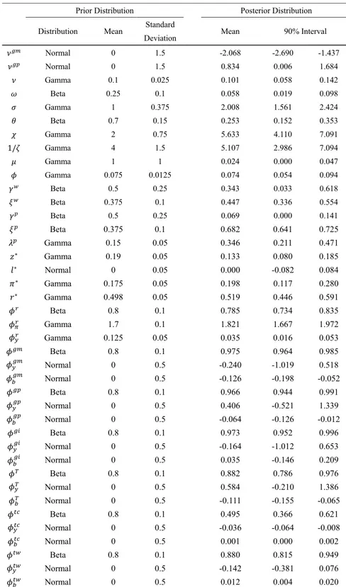
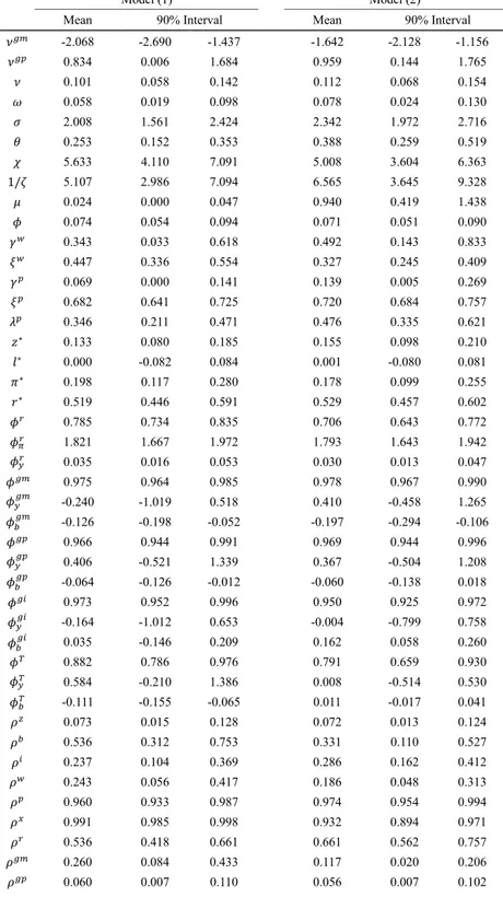
In this section, the parameters are estimated with a standard Bayesian estimation based on the Markov chain Monte Carlo (MCMC) method. Specifically, we can use the solution equations of the log-linearized model and observation equations linking the model variables to data to evaluate the log likelihood function using a Kalman filter. Further, combining the log likelihood with the prior distribution of parameters, we perform MCMC sampling on the basis of a Metropolis-Hastings algorithm to obtain the posterior distribution. We generate two Markov chains with 700,000 draws and discard the first 280,000 draws as burn-in draws.

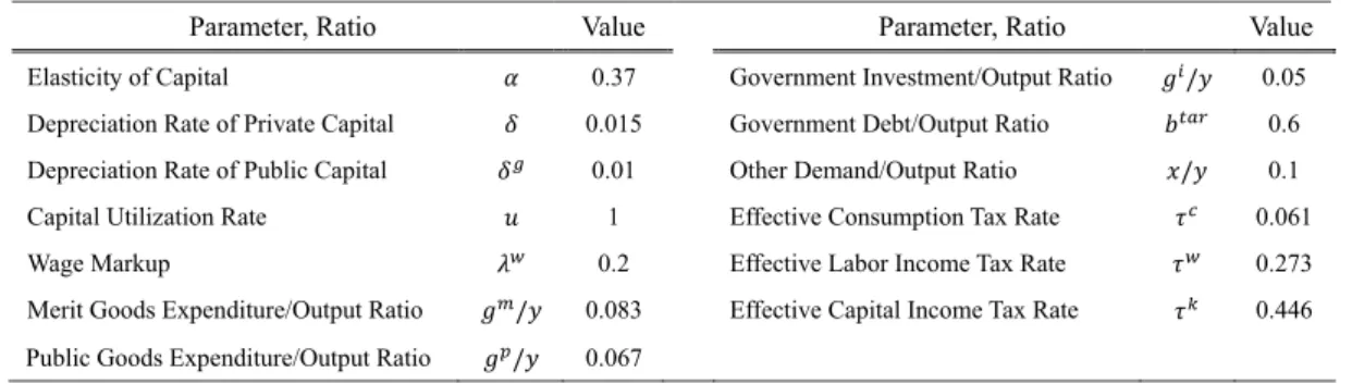
III-1. Data, Calibration, and Prior Distribution

In estimation, we employ thirteen quarterly data series from the first quarter of 1981 to the fourth quarter of 2012: real GDP, real private consumption, real private investment, real wages, real merit goods expenditure, real public goods expenditure, real government invest- ment, working hours, the inflation rate, the nominal interest rate, the effective consumption tax rate, the effective labor income tax rate, and effective capital income tax.

Series except tax rates are constructed in the same manner as Hirose (2012) and Kotera and Sakai (2017). For tax rates, effective tax rate series are created by following Mendoza, Razin, and Tesar (1994), Forni, Monteforte, and Sessa (2009), and Hasumi (2014). These data series are related to the endogenous variables of the model through the following obser- vation equation:

ΔlnY

ΔlnC ΔlnI

ΔlnW

ΔlnG

ΔlnG

ΔlnG

ΔlnP

lnR

τ

τ

τ

lnl

z

＋z

z

＋z

z

＋z

z

＋z

z

＋z

z

＋z

z

＋z

r

＋π

100τ

100τ 100τ

π l

y

－y

c

－c

w

－w

i

－i

l

π

r

τ

τ

τ

－

＝

－

－

┌│

││

││

││

││

││

││

││

││

││

││

└

┌│

││

││

││

││

││

││

││

││

││

││

└

┌│

││

││

││

││

││

││

││

││

││

││

└

┌│

││

││

││

││

││

││

││

││

││

││

└

┌│

││

││

││

││

││

││

││

││

││

││

└

＋

┌│

││

││

││

││

││

││

││

││

││

││

└

ɡ ɡ

ɡ ɡ

ɡ ɡ

～ ～

～ ～

～ ～

～ ～

～ ～

～ ～

～ ～

～

～

～

～

～

～

(46)

where the small-letter notation with the tilde expresses the log-deviation of the de-trended

9 The effective tax rate series used in this study is calculated as the ratio of tax revenue to the tax base, using national accounts data. For consumption tax, social insurance fees are included in both individual consumption tax and labor income tax.