Economic Effects of the USA - China Trade War: CGE Analysis with the GTAP 9.0a Data Base

(1)

Economic Effects of the USA - China Trade War: CGE Analysis with the GTAP 9.0a Data Base

ENKHBAYAR Shagdar

Senior Research Fellow, Research Division, ERINA

Tomoyoshi NAKAJIMA

Senior Research Fellow, Research Division, ERINA December, 2018

Niigata, Japan

ECONOMIC RESEARCH INSTITUTE FOR NORTHEAST ASIA

ERINA Discussion Paper No.1806e

(2)

1

Economic Effects of the USA - China Trade War: CGE Analysis with the GTAP 9.0a Data Base

Enkhbayar Shagdar*

Tomoyoshi Nakajima**

Abstract

An analysis of the economic effects of the ongoing USA-China trade war using the standard CGE Model and GTAP Data Base 9.0a revealed that both parties will be worse-off from this trade friction, having welfare losses and real GDP contractions regardless of international capital mobility status—i.e. whether the capital is internationally mobile or not. Moreover, the results indicated that the negative economic and trade impacts on China would be larger compared to those of the USA. Although, other countries and regions would be better-off having positive changes in their welfare and real GDP, their magnitudes were much lower than losses of the USA and China. Therefore, as a whole, the global economy will be worse-off as a result of this trade war between the world’s two largest economies, the USA and China.

Keywords: Trade policy; CGE models JEL classification codes: F13; C68

1. The Model and Experiment

In analyzing the economic effects of the recent trade friction between the USA and China, we employed the Global Trade Analysis Project (GTAP) Data Base (Version 9.0a) and the standard GTAP Model (The Model). The GTAP Model is a multi-region and multi-sector Computable General Equilibrium (CGE) model

ⁱ

with perfect competition and constant returns to scale. Bilateral trade is handled via the Armington assumption. It combines detailed bilateral trade, transport and protection data characterizing the economic linkages among regions, together with individual country input–output databases, which account for inter-sectoral linkages.

The GTAP Data Base 9.0a has triple reference years (2004, 2007 and 2011) and this analysis used 2011 as the reference year. Thus the values indicated in this analysis are expressed in constant 2011 US$ terms. The data are for 140 regions and 57 commodities, and in the consideration of the target countries the regions were aggregated into 12 from the original 140 regions in the model, while the original 57 sectors in the model were not aggregated. The aggregated regions are: China, Japan, the ROK, Mongolia, Russia, the EAEU4, ASEAN9, ANZI, the Rest of Asia, the United States, the EU_28, and Rest of World. Due to lack of data, the DPRK was not included in the Northeast Asia region, but the country is included implicitly in the Rest of Asia region as a part of the Rest of East Asia. Thus, the NEA region in this analysis refers to five countries in the region, excluding the DPRK (Appendix Tables I and II).

The original eight factors in the Model were aggregated into four factors: land, labor, capital

(3)

2

and natural resources, where land and natural resources are immobile and labor and capital are mobile factors (Appendix Table III).

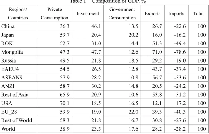
The composition of GDP of the countries in question is provided in Table 1. Structure of the economies in the GTAP database is based on individual country’s input-output table and its date varies by country. For example, the GTAP Data Base 9.a contains China’s 2010 input-output table of 45 sectors, while that of the USA is 2002 input-output table of 57 sectors. GDP shares of foreign trade activities of China were higher than those in the USA; thus the subsequent economy-wide effects of the recent trade friction between the two countries, so called “U.S.- China Trade War”, are expected to be more profound for China than its counterpart (Table 1).

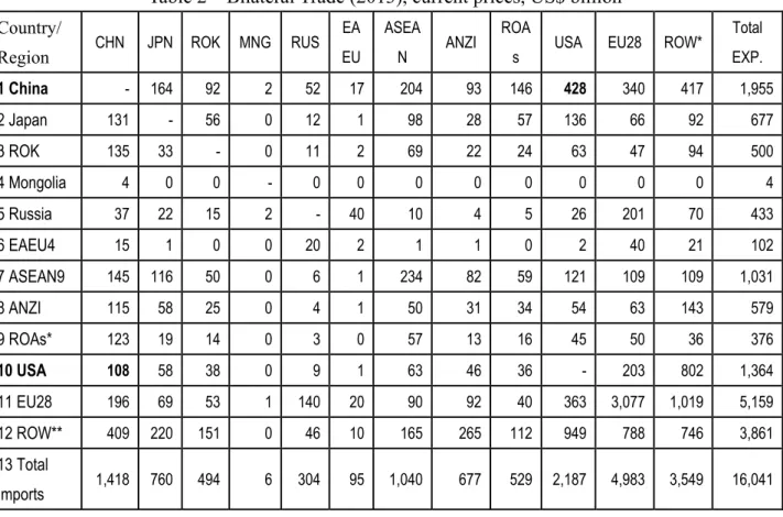
According to the database, China’s exports to the USA was much larger equaling to $428 billion or 21.9% of total in 2013 than the USA exports to China, which accounted for $108 billion or 7.9% of total. Therefore, the magnitude of the expected negative impacts of this trade friction would be much higher for China compared to that of the USA (Table 2).

Table 1 Composition of GDP, %

Regions/

Countries

Private

Consumption Investment Government

Consumption Exports Imports Total

China 36.3 46.1 13.5 26.7 -22.6 100

Japan 59.7 20.4 20.2 16.0 -16.2 100

ROK 52.7 31.0 14.4 51.3 -49.4 100

Mongolia 47.3 47.7 12.6 71.0 -78.6 100

Russia 49.5 21.8 18.5 29.2 -19.0 100

EAEU4 54.5 26.5 12.8 43.7 -37.4 100

ASEAN9 57.9 28.2 10.8 56.7 -53.6 100

ANZI 58.7 30.2 14.8 20.5 -24.2 100

Rest of Asia 65.9 20.9 10.6 53.8 -51.2 100

USA 70.1 18.5 16.5 12.1 -17.2 100

EU_28 59.9 19.0 22.0 39.3 -40.3 100

Rest of World 58.3 21.8 16.7 30.8 -27.6 100

World 58.9 23.5 17.6 28.2 -28.2 100

Source: GTAP 9.0a Data Base

(4)

3

Table 2 Bilateral Trade (2013), current prices, US$ billion

Country/

Region CHN JPN ROK MNG RUS EA

EU

ASEA

N ANZI ROA

s USA EU28 ROW* Total EXP.

1 China - 164 92 2 52 17 204 93 146 428 340 417 1,955

2 Japan 131 - 56 0 12 1 98 28 57 136 66 92 677 3 ROK 135 33 - 0 11 2 69 22 24 63 47 94 500 4 Mongolia 4 0 0 - 0 0 0 0 0 0 0 0 4 5 Russia 37 22 15 2 - 40 10 4 5 26 201 70 433 6 EAEU4 15 1 0 0 20 2 1 1 0 2 40 21 102 7 ASEAN9 145 116 50 0 6 1 234 82 59 121 109 109 1,031 8 ANZI 115 58 25 0 4 1 50 31 34 54 63 143 579 9 ROAs* 123 19 14 0 3 0 57 13 16 45 50 36 376

10 USA 108 58 38 0 9 1 63 46 36 - 203 802 1,364

11 EU28 196 69 53 1 140 20 90 92 40 363 3,077 1,019 5,159 12 ROW** 409 220 151 0 46 10 165 265 112 949 788 746 3,861 13 Total

Imports 1,418 760 494 6 304 95 1,040 677 529 2,187 4,983 3,549 16,041 Notes: *Rest of Asia; **Rest of World.

Source: GTAP 9.0a Data Base.

2. The Experiment

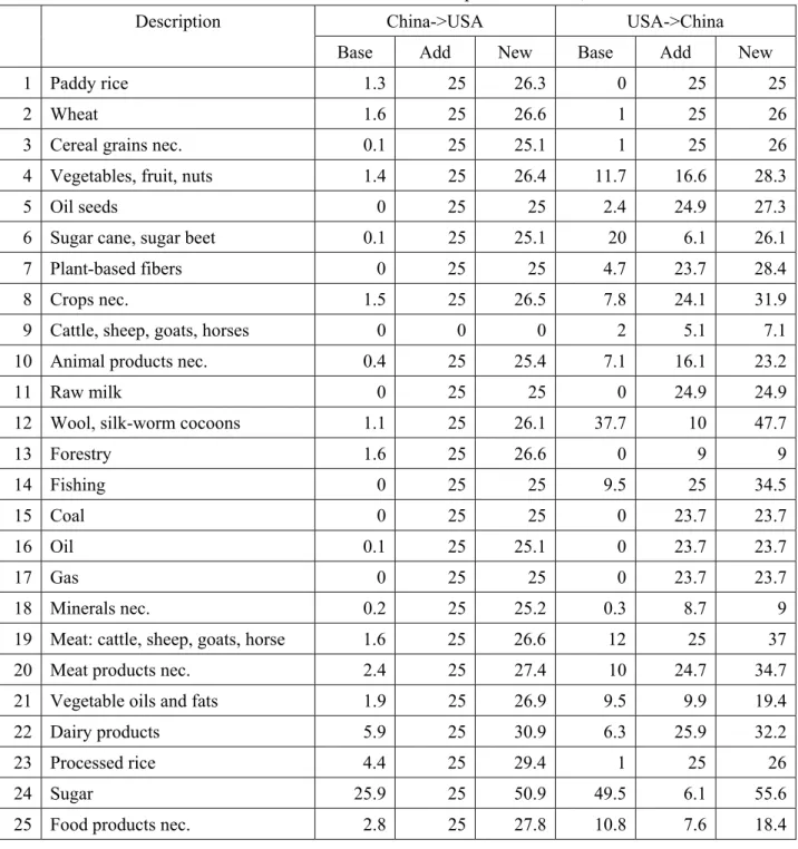
In September 2018, the Daiwa Institute of Research (DIR) released a report (Kobayashi, Sh, and Hirono, Y., 2018), where additional tariff rates associated with the latest USA-China trade war were estimated for 97 products classified by HS 2-Digits. In the GTAP model, source- specific tax on imports of commodity “i” from country “r” into country “s” is expressed by a variable “tms (i,r,s)” and the data base contains base rates for 42 traded commodities out of 57 commodities in the database, excluding utility, transport and service sectors (numbered from 43 to 57 in the Appendix Table II). Accordingly, the additional tariff rates for 42 traded commodities in GTAP database were computed based on the above mentioned DIR report and the scenario used in this experiment were as follow:

- The USA imposes 25% additional import tariffs on all traded commodities, except cattle, sheep, goats, horses (ctl) and wearing apparel (wap) originated from China; and

- China retaliates it with import tariff increases of 5.16% -25% on all 42 traded commodities originated from the USA.

The base and the computed additional tariff rates are provided in Table 3. The ad valorem

import tariffs expressed by a variable “tms (i,r,s)” in the Model were shocked to reach the new

target rates as provided in Table 3. Both values of the parameter “RORDELTA”, which is the

(5)

4

investment allocation binary coefficient in the Model, were applied in the scenario to observe the impacts of investment allocation decisions in the assumed trade war. The default value of the parameter RORDELTA in the Model equals 1, where investment is allocated across regions to equate the change in the expected rates of return, rore (r) which implies international capital mobility. When RORDELTA equals 0, investments are allocated across regions to maintain the existing composition of capital stock (no international capital mobility) and it effectively fixes the trade balance for each country/region. The solution method was Gragg, which is a multiple step extrapolation method.

Table 3 Base and New Bilateral Import Tax Rates, %

Description China->USA USA->China

Base Add New Base Add New

1 Paddy rice 1.3 25 26.3 0 25 25

2 Wheat 1.6 25 26.6 1 25 26

3 Cereal grains nec. 0.1 25 25.1 1 25 26

4 Vegetables, fruit, nuts 1.4 25 26.4 11.7 16.6 28.3

5 Oil seeds 0 25 25 2.4 24.9 27.3

6 Sugar cane, sugar beet 0.1 25 25.1 20 6.1 26.1

7 Plant-based fibers 0 25 25 4.7 23.7 28.4

8 Crops nec. 1.5 25 26.5 7.8 24.1 31.9

9 Cattle, sheep, goats, horses 0 0 0 2 5.1 7.1

10 Animal products nec. 0.4 25 25.4 7.1 16.1 23.2

11 Raw milk 0 25 25 0 24.9 24.9

12 Wool, silk-worm cocoons 1.1 25 26.1 37.7 10 47.7

13 Forestry 1.6 25 26.6 0 9 9

14 Fishing 0 25 25 9.5 25 34.5

15 Coal 0 25 25 0 23.7 23.7

16 Oil 0.1 25 25.1 0 23.7 23.7

17 Gas 0 25 25 0 23.7 23.7

18 Minerals nec. 0.2 25 25.2 0.3 8.7 9

19 Meat: cattle, sheep, goats, horse 1.6 25 26.6 12 25 37

20 Meat products nec. 2.4 25 27.4 10 24.7 34.7

21 Vegetable oils and fats 1.9 25 26.9 9.5 9.9 19.4

22 Dairy products 5.9 25 30.9 6.3 25.9 32.2

23 Processed rice 4.4 25 29.4 1 25 26

24 Sugar 25.9 25 50.9 49.5 6.1 55.6

25 Food products nec. 2.8 25 27.8 10.8 7.6 18.4

(6)

5

26 Beverages and tobacco products 4.1 25 29.1 6.1 18.6 24.7

27 Textiles 8.8 25 33.8 6.6 17.1 23.7

28 Wearing apparel 11.6 0 11.6 15.8 9.1 24.9

29 Leather products 13.5 25 38.5 7.9 10 17.9

30 Wood products 0.6 25 25.6 0.5 9 9.5

31 Paper products, publishing 0 25 25 1 6.5 7.5

32 Petroleum, coal products 0.2 25 25.2 3.9 23.7 27.6

33 Chemical, rubber, plastic products 2.7 25 27.7 6 7.9 13.9

34 Mineral products nec. 4.7 25 29.7 12.5 8.7 21.2

35 Ferrous metals 1 25 26 2.3 6.7 9

36 Metals nec. 3.2 25 28.2 1 7.1 8.1

37 Metal products 2.3 25 27.3 9.1 7.4 16.5

38 Motor vehicles and parts 0.9 25 25.9 22.4 23.8 46.2

39 Transport equipment nec. 3.4 25 28.4 2.6 5.5 8.1

40 Electronic equipment 0.3 25 25.3 0.7 8.5 9.2

41 Machinery and equipment nec. 1.5 25 26.5 4.8 7.8 12.6

42 Manufactures nec. 1.5 25 26.5 14.5 6.7 21.2

Note: nec. = not elsewhere classified.

3. The Results

a) Impacts on Welfare, Real GDP and Consumption

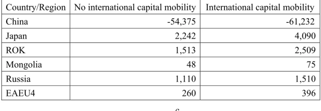
In terms of the equivalent variation (EV), which is an indicator for measuring the effect on public welfare, the simulation results demonstrated that both China and the USA would have welfare losses from the USA-China trade war regardless of the investment allocation decisions, while other countries and regions, including those in the NEA region, would experience welfare gains and real GDP expansions. The scale of welfare losses were much larger for China compared to those of the USA and the welfare losses of China would equal to US$54.4 billion without international capital mobility and to US$61.2 billion with international capital mobility, while those of the USA would account for US$21.2 billion and US$33.8 billion respectively.

At the same time, the EU_28 would have the largest welfare gain of US$5.6 billion and US$9.7 billion respectively without and with international capital mobility, while those for Japan and the ROK equaled to US$2.2 billion and US$1.5 billion, respectively. All other countries and regions would also benefit from welfare gains, but their magnitudes were much lower compared to welfare losses of China and the USA; thus making the global economy worse-off as a result of this trade war (Table 4).

Most of China’s welfare gain was associated with losses in terms of trade in goods and

services regardless of international investment allocation decisions and they equaled to

US$40.2 billion and US$46.3 billion respectively without and with international capital

(7)

6

mobility. Also, China’s allocative efficiency loss accounted for US$16.6 billion, when international capital is immobile, while it equaled to US$19.4 billion with international capital mobility. However, similar to the USA, China would gain in terms of trade in investment and services regardless of international investment allocation decisions. China’s terms of trade in investment and savings were improved by US$2.4 billion and US$4.5 billion respectively without and with international capital mobility. At the same time, for the USA, most of its welfare losses were associated with losses in allocative efficiency. Moreover, the USA would experience gains of US$6.7 billion in terms of trade in goods and services without international capital mobility, while it would result in losses of US$1.4 billion, when international capital is mobile (Tables 5).

In addition, the simulation results indicated that both the USA and China would have negative changes in their real GDP (expressed in the GDP quantity index) regardless of the investment allocation decisions. China’s real GDP contractions were slightly larger equaling 0.227% and 0.266% depending on the investment allocation decisions, while those for the USA were 0.217% and 0.224%. Higher values were observed when capital is internationally mobile (Table 6). Meanwhile, the DIR reported similar values for real GDP changes, when the USA raises its additional tariff rate to 25% and real GDP of China and the USA would contract by 0.22% and 0.28% respectively (Kobayashi, Sh, and Hirono, Y., 2018). Real GDP changes of all other countries and regions were positive in both scenarios, although at much lower scales compared to those of the USA and China.

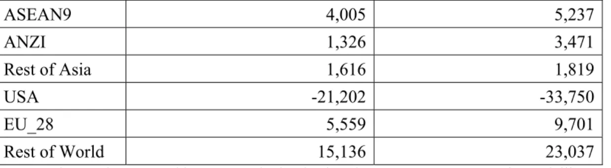
In terms of consumption, both the private and public consumptions of China would decrease regardless of investment allocation decisions and the scale of government consumption reductions were larger than drops in its private consumption. Reduction rates of consumption ranged between 2.7% and 3.3% depending on investment allocation decisions. At the same time, the USA may experience 02% decline in terms of government consumption, while private consumption in the country would raise by 0.3% regardless of investment allocation decisions. Consumption changes of all other countries and regions were positive and these values were higher when capital is internationally mobile (Table 7).

Table 4 Welfare Impacts of the USA-China Trade War: Equivalent Variation (EV), (2011 US$ Million)

Country/Region No international capital mobility International capital mobility

China -54,375 -61,232

Japan 2,242 4,090

ROK 1,513 2,509

Mongolia 48 75

Russia 1,110 1,510

EAEU4 260 396

(8)

7

ASEAN9 4,005 5,237 ANZI 1,326 3,471 Rest of Asia 1,616 1,819

USA -21,202 -33,750

EU_28 5,559 9,701 Rest of World 15,136 23,037

Source: The results reported here were obtained using the GEMPACK economic modelling software [Horridge et al. (2018)].

Table 5 Welfare Effects: EV Decomposition Summary of China and the USA

Components No international capital mobility

International capital mobility

China USA China USA

Allocative Efficiency

-16,597 -33,730 -19,388 -34,799

Terms of Trade in Goods and Services

-40,162 6,765 -46,327 -1,410

Terms of Trade in Investment and Savings

2,389 5,763 4,493 2,460

Total welfare -54,370 -21,202 -61,222 -33,750

Table 6 Real GDP Changes in the USA-China Trade War (qgdp = GDP quantity index) (% change)

Country/Region No international capital mobility International capital mobility

China

-0.227 -0.266

Japan

0.002 0.004

ROK

0.019 0.052

Mongolia

^0.028 ^0.109

Russia

0.022 0.029

EAEU4

0.014 0.026

ASEAN9

0.024 0.036

ANZI

^0.015 ^0.034

Rest of Asia

0.017 0.019

USA

-0.217 -0.224

EU_28

^0.01 ^0.01

Rest of World

^0.028 ^0.041

(9)

8

Table 7 USA-China Trade War Impacts on Consumption

(% change) Country/

Region

Private Consumption (yp) Government Consumption (yg) No international

capital mobility

International capital mobility

No international capital mobility

International capital mobility

China -2.7 -3.1 -2.9 -3.3

Japan 0.2 0.5 0.2 0.5

ROK 0.4 0.7 0.5 0.7

Mongolia 0.6 1.3 0.7 1.5

Russia 0.3 0.6 0.3 0.6

EAEU 0.2 0.5 0.3 0.6

ASEAN9 0.6 0.8 0.7 0.9

ANZI 0.3 0.6 0.3 0.6

Rest of Asia 0.4 0.4 0.4 0.5

USA 0.3 -0.2 0.3 -0.2

EU_28 0.3 0.4 0.3 0.4

Rest of World 0.7 0.9 0.7 0.9

Notes:

1. yp = Percentage change in regional private consumption expenditure in region r;

2. yg = Percentage change in regional government consumption expenditure in region r;

b) Impacts on Trade

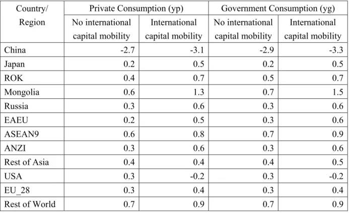
As mentioned earlier, China’s terms of trade would worsen as a result of the USA-China trade war regardless of investment allocation decisions. China may experience 2.102% decline in its terms of trade when international capital is immobile and it would equal to 2.405% with international capital mobility. At the same time, terms of trade of the U.S would improve by 0.355% without international capital mobility, while it would worsen by 0.075% with international capital mobility. The latter result indicates a contradictory outcome of the USA intension to improve its trade balance via the protectionary tariffs. Terms of trade of all other countries and regions had improved regardless of investment allocation decisions (Table 8).

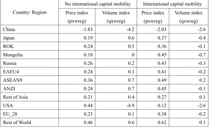
The simulation results indicated that both price and quantity of China’s merchandize

exports would decline from this trade war regardless of investment allocation decisions. The

magnitude of export price drop was higher at 2.03% when capital is internationally mobile and

thus, the scale of export quantity reduction was less at 2.6% compared to 4.2% without

international capital mobility. At the same time, export quantity or the real export (expressed

(10)

9

by the volume index, qxwreg) of the USA would also decline by due to increased prices regardless of investment allocation decisions. The magnitude of real export drop was lower at 2.6% when international capital is mobile. This indicates that along with more protected market of China, it would be difficult for the USA to increase its exports to other markets, whereas China was the second largest export market of the USA among the selected countries and regions. Real exports of most of other countries and regions may also experience declines with international capital mobility. The reduction rates ranged between 0.1% (the lowest) for the ROK and ANZI and 0.7% (the highest) for Mongolia (Tables 2 and 9).

Table 8 USA-China Trade War Impacts on Terms of Trade, % change Country/Region No international capital

mobility

International capital mobility

China -2.102 -2.405

Japan 0.275 0.443

ROK 0.265 0.352

Mongolia 0.752 1.030

Russia 0.246 0.345

EAEU4 0.277 0.379

ASEAN9 0.346 0.418

ANZI 0.190 0.349

Rest of Asia 0.249 0.268

USA 0.355 -0.075

EU_28 0.072 0.125

Rest of World 0.331 0.461

As expected, both China and the USA experienced drops in their imports due to price increases regardless of investment allocation decisions. With international capital mobility, the reductions were higher and the magnitude of China’s import quantity decline was higher at 6.4% compared to that of the USA Import quantity of all other countries and regions had increases regardless of price movements and investment allocation decisions (Table 9).

Without international capital mobility, magnitude of the USA export quantity drop (4.9%)

was larger than that of its import (3.1%), whereas the USA has huge trade deficit. Thus,

effectiveness of the USA protectionary tariff policy might not be sufficient for addressing this

issue and the USA needs to seek opportunities for expanding its export markets (Tables 9 & 10).

(11)

10

Table 9 USA-China Trade War Effects on Exports

(% change)

Country/ Region

No international capital mobility International capital mobility Price index

(pxwreg)

Volume index (qxwreg)

Price index (pxwreg)

Volume index (qxwreg)

China -1.83 -4.2 -2.03 -2.6

Japan 0.19 0.6 0.37 -0.4

ROK 0.24 0.5 0.36 -0.1

Mongolia 0.18 0 0.45 -0.7

Russia 0.26 0.2 0.43 -0.3

EAEU4 0.24 0.1 0.41 -0.2

ASEAN9 0.36 0.7 0.49 0.2

ANZI 0.24 0.7 0.45 -0.1

Rest of Asia 0.21 0.4 0.27 0.1

USA 0.44 -4.9 0.12 -2.6

EU_28 0.23 0.1 0.38 -0.2

Rest of World 0.46 0.6 0.62 0.1

Notes: 1. pxwreg = percentage change in price index of merchandise exports by region;

2. qxwreg = percentage change in volume of merchandise exports by region;

Table 10 USA-China Trade War Effects on Imports

(% change) No international capital mobility International capital mobility

Price index (piwreg)

Volume index (qiwreg)

Price index (piwreg)

Volume index (qiwreg)

China 0.28 -5.8 0.39 -6.4

Japan -0.09 0.7 -0.07 1.0

ROK -0.02 0.6 0.01 0.7

Mongolia -0.56 0.2 -0.57 1.1

Russia 0.01 0.3 0.09 0.9

EAEU4 -0.04 0.2 0.03 0.5

ASEAN9 0.02 0.8 0.07 1.0

ANZI 0.05 0.4 0.1 0.8

Rest of Asia -0.04 0.6 0.0 0.7

USA 0.09 -3.1 0.2 -4.1

EU_28 0.16 0.1 0.25 0.3

(12)

11

Rest of World 0.13 0.7 0.16 1.1

Notes:

1. piwreg = percentage change in price index of merchandise imports by region;

2. qiwreg = percentage change in volume of merchandise imports by region;

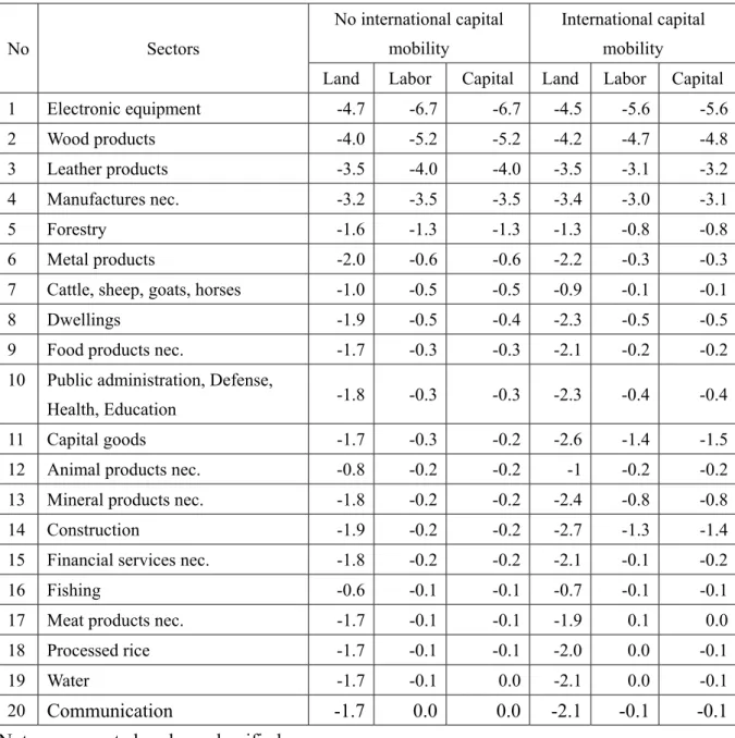
c) Impacts on China’s Industry

As the simulation results indicate, there will be both loser and winner industries as a result of the USA-China trade war. But, the number of contracting sectors (20 losers) were smaller than that of expanding (38 winners) industries. With international capital mobility, the magnitude of output drops of the contracting (losing) industries was lower, while the scale of expanding (winning) industries was higher. This may suggest that this trade war might be an opportunity for China to increase its industrial output by expanding its domestic and other foreign markets.

China’s electronic equipment production drop was the highest among the contracting industries and its output may see 6.7% and 5.6% reductions with and without international capital mobility respectively. Wood and leather products were the next largest contracting sectors and their output would decline in a range of 3.2% to 5.2% depending on investment allocation decisions. Accordingly, demand for endowments (land, labor, capital) of these sectors dropped at similar rates to output declines. For example, demand for labor and capital in electronic equipment production reduced by 6.7% each without international capital mobility and the drops equaled 5.6% each when international capital is mobile. Therefore, it would be appropriate for China to introduce policies, such as training and re-training programs, as a countermeasure of employment loss from this trade war (Tables 11 & 13).

However, substantial number of industries in China may benefit from the USA-China trade war by increasing their outputs. The magnitude of output expansions were larger when international capital is mobile. Plant-based fibers, oil seeds, wearing apparel and wool, silk- worm cocoons were top winners among the expanding industries and the scales of output expansions of these leading industries ranged between 4.0% and 7.5% depending on investment allocation decisions. Along with output expansions, demands for production factors would also increase and their magnitude varied depending on their factor intensities. For example, demands for labor and capital for plant-based fibers, oil seeds and wool, silk-worm cocoons would raise in a range of 4.5% and 8.3% depending on investment allocation decisions, while their demands for land would increase at lower than these rates ranging between 2.9% and 5.7% (Tables 12 &

14).

(13)

12

Table 11 USA-China Trade War Effects on China’s Industrial Output, [%-change]: Losers

No Sectors No international capital

mobility

International capital mobility

1 Electronic equipment -6.7 -5.6

2 Wood products -5.2 -4.8

3 Leather products -4.0 -3.2

4 Manufactures nec. -3.5 -3.1

5 Forestry -1.2 -0.7

6 Cattle, sheep, goats, horses -0.7 -0.3

7 Metal products -0.6 -0.3

8 Dwellings -0.4 -0.5

9 Animal products nec. -0.3 -0.5

10 Food products nec. -0.3 -0.2

11 Public administration, Defense,

Health, Education -0.3 -0.4

12 Capital goods -0.3 -1.4

13 Mineral products nec. -0.2 -0.8

14 Construction -0.2 -1.3

15 Financial services nec. -0.2 -0.1

16 Fishing -0.1 -0.1

17 Meat products nec. -0.1 0.1

18 Processed rice -0.1 0.0

19 Water -0.1 -0.1

20 Communication 0.0 -0.1

Note: nec.= not elsewhere classified;

Table 12 USA-China Trade War Effects on China’s Industrial Output, [%-change]: Winners

No Sectors No international

capital mobility

1 Plant-based fibers 6.6 7.5

2 Oil seeds 5.5 5.9

3 Wearing apparel 4.1 4.8

4 Wool, silk-worm cocoons 4.0 5.2

(14)

13

5 Transport equipment nec. 3.7 3.7

6 Crops nec. 2.4 3.1

7 Metals nec. 2.1 2.7

8 Textiles 1.8 2.6

9 Minerals nec. 1.6 1.8

10 Meat: cattle, sheep, goats, horse 1.6 2.0

11 Oil 1.2 1.4

12 Motor vehicles and parts 1.1 0.7

13 Air transport 1.1 1.3

14 Sugar 1.0 1.2

15 Chemical, rubber, plastic products 1.0 1.5

16 Sugar cane, sugar beet 0.9 1.1

17 Coal 0.8 0.9

18 Ferrous metals 0.8 0.7

19 Gas 0.7 0.8

20 Dairy products 0.7 0.7

21 Machinery and equipment nec. 0.6 0.8

22 Insurance 0.6 0.7

23 Cereal grains nec. 0.5 0.7

24 Raw milk 0.5 0.5

25 Paper products, publishing 0.4 0.7

26 Petroleum, coal products 0.4 0.5

27 Electricity 0.4 0.5

28 Business services nec. 0.4 0.2

29 Wheat 0.3 0.4

30 Vegetable oils and fats 0.3 0.5

31 Transport nec. 0.3 0.1

32 Paddy rice 0.2 0.3

33 Vegetables, fruit, nuts 0.2 0.3

34 Trade 0.2 0.2

35 Sea transport 0.2 0.3

36 Gas manufacture, distribution 0.1 0.1

37 Recreation and other services 0.1 0.0

38 Beverages and tobacco products 0.0 0.0

Note: nec.= not elsewhere classified;

(15)

14

Table 13 USA-China Trade War Impacts on Demand for Endowments for use in China’s Industry, % Change: Contracting Industries

No Sectors

No international capital mobility

Land Labor Capital Land Labor Capital

1 Electronic equipment -4.7 -6.7 -6.7 -4.5 -5.6 -5.6

2 Wood products -4.0 -5.2 -5.2 -4.2 -4.7 -4.8

3 Leather products -3.5 -4.0 -4.0 -3.5 -3.1 -3.2

4 Manufactures nec. -3.2 -3.5 -3.5 -3.4 -3.0 -3.1

5 Forestry -1.6 -1.3 -1.3 -1.3 -0.8 -0.8

6 Metal products -2.0 -0.6 -0.6 -2.2 -0.3 -0.3

7 Cattle, sheep, goats, horses -1.0 -0.5 -0.5 -0.9 -0.1 -0.1

8 Dwellings -1.9 -0.5 -0.4 -2.3 -0.5 -0.5

9 Food products nec. -1.7 -0.3 -0.3 -2.1 -0.2 -0.2

10 Public administration, Defense,

Health, Education -1.8 -0.3 -0.3 -2.3 -0.4 -0.4

11 Capital goods -1.7 -0.3 -0.2 -2.6 -1.4 -1.5

12 Animal products nec. -0.8 -0.2 -0.2 -1 -0.2 -0.2

13 Mineral products nec. -1.8 -0.2 -0.2 -2.4 -0.8 -0.8

14 Construction -1.9 -0.2 -0.2 -2.7 -1.3 -1.4

15 Financial services nec. -1.8 -0.2 -0.2 -2.1 -0.1 -0.2

16 Fishing -0.6 -0.1 -0.1 -0.7 -0.1 -0.1

17 Meat products nec. -1.7 -0.1 -0.1 -1.9 0.1 0.0

18 Processed rice -1.7 -0.1 -0.1 -2.0 0.0 -0.1

19 Water -1.7 -0.1 0.0 -2.1 0.0 -0.1

20

Communication -1.7 0.0 0.0 -2.1 -0.1 -0.1

Note: nec.= not elsewhere classified;

Table 14 USA-China Trade War Impacts on Demand for Endowments for use in China’s Industry, % Change: Expanding Industries

No Sectors

No international capital mobility

Land Labor Capital Land Labor Capital

1 Plant-based fibers 5.0 7.2 7.2 5.7 8.3 8.3

2 Oil seeds 4.1 6.1 6.1 4.3 6.6 6.6

(16)

15

3 Wool, silk-worm cocoons 2.9 4.5 4.5 3.7 5.8 5.8

4 Wearing apparel 0.1 4.1 4.2 0 4.8 4.7

5 Transport equipment nec. -0.1 3.7 3.7 -0.5 3.7 3.7

6 Gas 2.1 3.2 3.2 2.3 3.6 3.6

7 Crops nec. 1.5 2.8 2.8 2.0 3.6 3.6

8 Metals nec. -0.8 2.1 2.1 -0.9 2.7 2.6

9 Oil 1.2 2.0 2.0 1.3 2.3 2.3

10 Minerals nec. 1.1 2.0 2.0 1.2 2.2 2.2

11 Textiles -0.9 1.8 1.8 -1.0 2.6 2.6

12 Meat: cattle, sheep, goats, horse -0.9 1.6 1.6 -1.0 2.0 2.0

13 Coal 0.7 1.4 1.4 0.7 1.6 1.6

14 Sugar cane, sugar beet 0.2 1.1 1.1 0.3 1.4 1.4

15 Motor vehicles and parts -1.2 1.1 1.1 -1.8 0.7 0.7

16 Air transport -1.5 1.1 1.1 -1.9 1.3 1.2

17 Chemical, rubber, plastic

products -1.3 1.0 1.0 -1.4 1.5 1.5

18 Sugar -1.2 0.9 1.0 -1.4 1.2 1.1

19 Ferrous metals -1.4 0.8 0.8 -1.8 0.8 0.7

20 Cereal grains nec. -0.1 0.7 0.7 0 1 0.9

21 Raw milk -0.1 0.7 0.7 -0.1 0.8 0.8

22 Dairy products -1.3 0.7 0.7 -1.6 0.7 0.7

23 Machinery and equipment nec. -1.5 0.6 0.6 -1.7 0.8 0.8

24 Insurance -1.4 0.6 0.7 -1.8 0.7 0.6

25 Wheat -0.2 0.5 0.5 -0.3 0.6 0.6

26 Paddy rice -0.4 0.4 0.4 -0.4 0.5 0.5

27 Vegetables, fruit, nuts -0.3 0.4 0.4 -0.4 0.5 0.5

28 Paper products, publishing -1.5 0.4 0.4 -1.8 0.7 0.7

29 Petroleum, coal products -1.5 0.4 0.4 -1.9 0.5 0.5

30 Electricity -1.5 0.4 0.4 -1.9 0.5 0.5

31 Business services nec. -1.5 0.4 0.4 -2.0 0.3 0.2

32 Vegetable oils and fats -1.5 0.3 0.3 -1.7 0.5 0.5

33 Transport nec. -1.8 0.3 0.3 -2.3 0.1 0.1

34 Trade -1.8 0.2 0.3 -2.2 0.3 0.2

35 Sea transport -1.9 0.2 0.2 -2.2 0.3 0.2

36 Gas manufacture, distribution -1.7 0.1 0.1 -2.0 0.1 0.1

37 Recreation and other services -1.7 0.1 0.1 -2.1 0 0

38 Beverages and tobacco products -1.6 0 0 -2.0 0 -0.1

(17)

16

Note: nec.= not elsewhere classified;

3. Conclusion

CGE analysis of the economic impacts of the recent USA-China trade war using GTAP Model and Data Base 9.0a has demonstrated that the protectionary bilateral tariff escalations in the USA and China would be harmful for both parties of this trade friction due to reduced trade and economic activities. Specifically:

•

Both the USA and China will be worse off as a result of the “trade war” (negative EV values and real GDP drops) regardless of whether capital is internationally mobile or not;

•

These welfare losses were associated with losses of allocative efficiency and terms of trade in goods and services when capital is internationally mobile, while the USA would have some gains (US$6.8 billion or 0.36%) in terms-of-trade in goods and services without international capital mobility;

•

China’s both private and government consumption expenditures would decline as a result of the “trade war” regardless of whether capital is internationally mobile or not, while those of the USA may have slight increases (0.3%) without international capital mobility;

•

China’s merchandise imports and exports would experience declines regardless of whether capital is internationally mobile or not;

•

There will be both “loser” and “winner” industries in China from this “trade war”.

•

Although other countries and regions may benefit from this trade friction by having positive changes in their welfare and real GDP and trade expansion. But, their magnitudes were much lower compared to negative economic impacts on the USA and China. Therefore, the global economy will be worse off as a result of this trade war between the world’s two largest economies, the USA and China.

*Senior Research Fellow, Research Division, ERINA

** Senior Research Fellow, Research Division, ERINA

i For more details on the GTAP model and database, refer to Hertel, T. (ed.), 1997.

References

ADAMS, Philip D. (2003

).

Interpretation of Macroeconomic Results from a CGE Model such as GTAP, Centre of Policy Studies, Monash University. Available online

.

BEGG, M., Ch. BURMAA, et al (2012). “GTAP 8 Data Base Documentation - Chapter 7.C:

(18)

17

Mongolia” by BEGG, Michael, BURMAA Chadraaval, RAGCHAARSUREN Galindev, ESMEDEKH Lkhanaajav, and ERDENESAN Eldev-Ochir. Retrieved from:

https://www.gtap.agecon.purdue.edu

ENKHBAYAR Shagdar and OTGONSAIKHAN Nyamdaa (2017). Impacts of Import Tariff Reforms on Mongolia’s Economy: CGE Analysis with the GTAP 8.1 Data Base, The Northeast Asian Economic Review, Vol. 5, No. 1, March 2017, pp. 1–25

ENKHBAYAR Shagdar and Tomoyoshi NAKAJIMA (2013). Impacts of Mongolian FTAs with the Countries in Northeast Asia: CGE Analysis with the GTAP 8 Data Base. The Northeast Asian Economic Review, Vol. 1, No. 2, December 2013, pp. 43–67.

HERTEL, T. (ed.) (1997). Global Trade Analysis: Modeling and Applications. Cambridge University Press

HORRIDGE J.M., JERIE M., MUSTAKINOV D. & SCHIFFMANN F. (2018), GEMPACK manual, GEMPACK Software, ISBN 978-1-921654-34-3

KOBAYASHI, Shunsuke and HIRONO, Yota (2018). Latest in US-China Trade War: Thorough analysis on additional tariff by product. Daiwa Institute of Research, 21 September 2018.

Available:

https://www.dir.co.jp/english/research/report/analysis/20180921_020329.html (October

15, 2018)

NAKAJIMA, Tomoyoshi (2012

). “The ROK’s FTA Policy: Developments under the Lee Myung- bak Administration”, The Journal of Econometric Study of Northeast Asia, Vol. 8, No. 2, 2012

NARAYANAN, G. Badri, Angel AGUIAR, and Robert McDOUGALL (eds.) (2012). Global

Trade, Assistance, and Production: The GTAP 8 Data Base, Center for Global Trade

Analysis, Purdue University

(19)

18

Appendix Table I: Classification of Regions in the Model

The Model

(12 regions)

GTAP 9.0a (140 regions)

China China

Japan Japan

ROK Republic of Korea Mongolia Mongolia

Russia Russian Federation

EAEU4 Kazakhstan, Kyrgyzstan, Armenia, Belarus

ASEAN9 ASEAN9 members, except Myanmar: Brunei Darussalam, Cambodia, Indonesia, Lao People's Democratic Republic, Malaysia, Philippines, Singapore, Thailand, Vietnam

ANZI Australia, New Zealand, India

Rest of Asia Hong Kong, Taiwan, Rest of East Asia, Rest of Southeast Asia, Bangladesh, Nepal, Pakistan, Sri Lanka, Rest of South Asia

USA United States of America

EU_28 Austria, Belgium, Cyprus, Czech Republic, Denmark, Estonia, Finland, France, Germany, Greece, Hungary, Ireland, Italy, Latvia, Lithuania, Luxembourg, Malta, Netherlands, Poland, Portugal, Slovakia, Slovenia, Spain, Sweden, United

Kingdom, Bulgaria, Romania, Croatia

Rest of World Rest of Oceania, Canada, Mexico, Rest of North America, Argentina, Bolivia, Brazil, Chile, Colombia, Ecuador, Paraguay, Peru, Uruguay, Venezuela, Rest of South America, Costa Rica, Guatemala, Honduras, Nicaragua, Panama,

El Salvador, Rest of Central America, Dominican Republic, Jamaica, Puerto Rico, Trinidad and Tobago, Caribbean, Switzerland, Norway, Rest of EFTA, Albania, Ukraine, Rest of Eastern Europe, Rest of Europe, Rest of Former Soviet Union, Azerbaijan, Georgia, Bahrain, Islamic Republic of Iran, Israel, Jordan, Kuwait, Oman, Qatar, Saudi Arabia, Turkey, United Arab Emirates, Rest of Western Asia, Egypt, Morocco, Tunisia, Rest of North Africa, Benin, Burkina Faso, Cameroon, Côte d'Ivoire, Ghana, Guinea, Nigeria, Senegal, Togo, Rest of Western Africa, Central Africa, South Central Africa, Ethiopia, Kenya, Madagascar, Malawi, Mauritius, Mozambique, Rwanda, Tanzania, Uganda, Zambia, Zimbabwe, Rest of Eastern Africa, Botswana, Namibia, South Africa, Rest of South African Customs, Rest of the World

(20)

19

Appendix Table II: Classification of Sectors in the Model

No. Code Description

1 pdr Paddy rice

2 wht Wheat

3 gro Cereal grains nec.

4 v_f Vegetables, fruit, nuts 5 osd Oil seeds

6 c_b Sugar cane, sugar beet 7 pfb Plant-based fibers 8 ocr Crops nec.

9 ctl Cattle, sheep, goats, horses 10 oap Animal products nec.

11 rmk Raw milk

12 wol Wool, silk-worm cocoons 13 frs Forestry

14 fsh Fishing

15 coa Coal

16 oil Oil

17 gas Gas

18 omn Minerals nec.

19 cmt Meat: cattle, sheep, goats, horse 20 omt Meat products nec.

21 vol Vegetable oils and fats 22 mil Dairy products

23 pcr Processed rice

24 sgr Sugar

25 ofd Food products nec.

26 b_t Beverages and tobacco products 27 tex Textiles

28 wap Wearing apparel 29 lea Leather products 30 lum Wood products

31 ppp Paper products, publishing 32 p_c Petroleum, coal products

33 crp Chemical, rubber, plastic products 34 nmm Mineral products nec.

35 i_s Ferrous metals 36 nfm Metals nec.

37 fmp Metal products

38 mvh Motor vehicles and parts 39 otn Transport equipment nec.

(21)

20

Appendix Table II: Classification of Sectors in the Model (continued)

No. Code Description

40 ele Electronic equipment

41 ome Machinery and equipment nec.

42 omf Manufactures nec.

43 ely Electricity

44 gdt Gas manufacture, distribution

45 wtr Water

46 cns Construction

47 trd Trade

48 otp Transport nec.

49 wtp Sea transport 50 atp Air transport 51 cmn Communication 52 ofi Financial services nec.

53 isr Insurance

54 obs Business services nec.

55 ros Recreation and other services

56 osg Public administration, Defense, Health, Education 57 dwe Dwellings

Appendix Table III: Classification of Production Factors in the Model

Old factor New factor

No. Code Description No. Code Description

1 Land Land 1 Land -1

2 tech_aspros Technicians/Associates, Professional 2 Labor mobile

3 clerks Clerks 2 Labor mobile

4 service_shop Service/Shop workers 2 Labor mobile 5 off_mgr_pros Officials and Managers 2 Labor mobile 6 ag_othlowsk Agricultural and Unskilled 2 Labor mobile