Flexibility of Design Variables to Pareto-Optimal Solutions in Multi Objective Optimization Problems

Flexibility of Design Variables to Pareto-Optimal Solutions in Multi Objective Optimization Problems

Tomoyuki HIROYASU, Shinpei CHINO, Mitsunori MIKI

Abstract— In this paper, we propose the concept of the flex- ibility of design variables to Pareto-optimal solutions in Multi- Objective Optimization problems. In addition, we introduce a method for measurement of the flexibility of design variables to Pareto-optimal solutions. Increases in the number of design variables usually result in a wide variety of optimum solutions.

However, when the flexibilities of some design variables are small, the contributions of these design variables are also very small. This means that the same Pareto-optimal solutions can be derived without these parameters. Therefore, it is very important to find the flexibility of the design variables to the Pareto-optimal solutions. To find the flexibility, the values of one of the design variables are changed, while those of the remaining parameters are fixed. In this procedure, it is very important to determine the fixed values. We describe these procedures to determine the flexibility of the design variable to the Pareto-optimal solutions. Finally, we illustrate using the diesel engine fuel emission scheduling problem that the Pareto- optimal solutions can be derived with only the design variables whose flexibilities are high.

I. I NTRODUCTION

Recently, systems with inner variables that can change their characteristics dynamically have attracted a great deal of attention. These H flexible systems Ican adapt to changes in the environment and are applicable to the needs of various users.

To illustrate flexible systems, the procedures used in the design of diesel engines are discussed. Diesel engines have good fuel efficiency and good carbon dioxide exhaust characteristics. For these reasons, diesel engines are widely used especially in commercial applications. However, diesel engines have disadvantages in that they produce high levels of NOx and soot in the exhaust. Many researchers and devel- opers are attempting to solve these problems. In conventional engines, the driving pattern of diesel engines is static and cannot be changed dynamically during driving. Therefore, the combustion forms are almost the same even when the engine is in a high speed static run and running on a slope.

Some diesel engine parameters, such as swirl ratio, fuel start angle, and fuel shape, can be changed by electronic control during driving. These changes also alter the characteristics of diesel engines. Thus, control of these parameters allows the fuel efficiency and the amounts of NOx and soot to be changed. When diesel engines are designed as flexible systems, these characteristics can be changed along with

T. Hiroyasu is with the Department of Engineering, Doshisha University 610-0321 Kyoto, Japan (email: [email protected]).

S. Chino is with the Graduate School of Engineering, Doshisha University 610-0321 Kyoto, Japan (email: [email protected]).

M. Miki is with the Department of Engineering, Doshisha University 610-0321 Kyoto, Japan (email: [email protected]).

Fig. 1. Trade-off between NOx and Soot

environmental changes and the driver Gs needs. As a result, the best combustion conditions can be chosen for the driving environment. Fuel efficiency is important when driving on the highway. The parameters of engines are shifted to values that confer high fuel efficiency on the engine. On the other hand, when the driver feels that the engine needs high power, the parameters can be changed. In this way, the design of engines as flexible systems can be both useful and convenient. For the design of flexible systems, it is important to find parameters that confer high flexibility on the characteristics.

In our sequential studies, we introduced the concept of flexible systems and proposed a method for the design of flexible systems. Flexible systems are especially effective in multidisciplinary designs, such as mechanical structure, con- trol, circular design, and software development. Therefore, there are several evaluate criteria in target design problems.

Generally, it is impossible to satisfy all of these criteria or optimize these functions at the same time. For example, the evaluation functions in diesel engine design are the fuel efficiency and the amounts of NOx and soot. It is better to design diesel engines that have high fuel efficiency and produce small amounts of NOx and soot. However, it is impossible to maximize and minimize these values at the same time, as there is a tradeoff relation between fuel efficiency, NOx, and soot, as described in Fig. 1.

In this paper, we describe the new concept of flexibility, which evaluates the flexibility of the design variables not to functions but to the Pareto-optimal solutions. The Pareto- optimal solutions are derived with design variables. However, when the flexibilities of some design variables are high, while those of others are low, and the same Pareto-optimal solutions are derived with parameters whose flexibilities are high. Only one of the design variables is needed if the ranges of the flexibilities of two design variables are almost the same.

Evaluation of the flexibility of design variables to Pareto-

optimal solutions is not easy. Here, we introduce a method for evaluation of the flexibility based on the diesel engine fuel emission scheduling problem.

II. M ULTI -O BJECTIVE O PTIMIZATION

A. Multi-Objective Optimization Problems

In the optimization problems, when there are several objective functions, the problems are called Multi-objective Optimization Problems (MOPs) [1]. Multi-objective opti- mization problems are formulated as follows,

8

<

:

min(max)

!

x);f

2 (

!

x);:::;f

k (

!

x)) T

subject to

jg

i (

!

x)0;(i=1;:::;m)g

(1)

In these equations,

;x

2

;:::;x

n )

T

is

th vector decision parameter.

indicates feasible region.

f

i (

!

x)=f

i (x

1

;x

2

;:::;x

n

);i=1;:::;k

g

j (

!

x)=g

j (x

1

;x

2

;:::;x

n

);j=1;:::;m

(2) Usually these objectives cannot minimize or maximize at the same time, since there is a trade off relation ship between the objectives. Therefore, one of the goals of multi-objective optimization problem is find a set of Pareto-optimum solu- tions.

B. Pareto-optimum solutions

Pareto-optimum solutions are defined using the concept of the domination of the solutions. The definitions of the dom- ination and non-nomination in multi-objective optimization problems are defined as follows.

The definition of the domination of the solutions:

x 1

;x 2

2F(x=(x

1

;x

2

;:::;x

n

))

is assumed.

1) When

,

is superior to

. 2) When

,

is superior to

in the

strong manner.

If

is superior to

,

is better than

. In the multi objective optimization problems, the solutions that are superior to the other solutions are searched. The definition of the Pareto solutions can be explained as follows.

The definition (The Pareto optimum sotluions):

F(x=(x

1

;x

2

;:::;x

n

))

is assumed.

1) There is no solution

that are superior to

in strong manner,

is called Pareto optimum solution.

2) There is no solution

that are superior to

,

x

0

is called weak Pareto optimum solution.

In Fig. 2, the example of the Pareto optimum solutions in the case of two objectives

is illustrated. In this figure, strong line shows the Pareto optimum solutions and dot line shows the weak Pareto optimum solutions.

Generally, there are plural Pareto optimum solutions are existed. To derive these optimum solutions set with one calculation trial, Multi Objective Genetic Algorithms are often used [2], [3], [4], [5], [6], [7].

Fig. 2. Pareto Optimal Solution and Feasible Region

Fig. 3. Description of one-pulse injection shape

III. T HE D IESEL E NGINE F UEL E MISSION S CHEDULING

P ROBLEM

A. Outline of the diesel engine fuel emission scheduling problem

In this study, a diesel engine was designed to minimize the amounts of SFC, NOx, and soot. SFC is an index minimization of which is associated with maximization of fuel economy. There are many design parameters for the diesel engine. In this study, we did not address shape parameters, such as bore diameter and stroke length, but targeted parameters that can be controlled electronically, such as EGR, swirl rate, and fuel injection ratio. The target shape parameter is related to physical size and is predetermined by the specification, and the degree of design freedom is low. On the other hand, parameters that can be controlled electronically are controllable or are new technologies that are becoming controllable, and will be used for engines in the near future. By targeting parameters that can be controlled electronically, the designed engine will not have one fixed solution but will have a dynamic design that can be adapted according to requirements. This is a so-called, flexible system, and will also be one of the forms of future engine design.

In this study, the amounts of SFC, NOx, and soot were used as the objective function, and we attempted to minimize them simultaneously. As shown in Fig. 3, the injection shape of the fuel is one-step injection where the fuel is injected in a single pulse.

Design Variables used here are StartAngle, Exhaust Gas

Recirculation (EGR), Boost Pressure, Swirl Ratio, and Inter-

val Angle.

B. HIDECS

The simulation of a diesel engine is very complicated.

Therefore, many models of diesel engine combustion have been proposed. These models can be classified into two categories: phenomenological models and detailed multi- dimensional models. Over the past 30 years, the most sophisticated phenomenological spray-combustion model, HIDECS, has shown great potential as a predictive tool for both performance and emissions in a wide range of direct injection diesel engines. This model was developed originally at the University of Hiroshima and was named FHIDECSGonly recently. A detailed discussion of this model and examples of its successful application are given in the references[8], [9], [10], [11], [12], [13], [14]. In this study, HIDECS was used as an analyzer to determine the target function values in optimization.

In HIDECS, the required calculation load is very light.

KIVA code of a detailed multi-dimensional model is a well- known diesel engine combustion analyzer; however, this model requires a very large calculation load for analysis for one trial. The genetic algorithm used in the present study exhibits high optimum solution search ability. The downside is that the calculations must be repeated many times. However, HIDECS allows use of the genetic algorithm within a practical time frame.

IV. F LEXIBILITY OF DESIGN VARIABLES

In this section, the concept of design variable flexibility is described. Then, the method for measurement of the flexibility is introduced. For simplicity, we focus on a multi- objective problem-the Diesel Engine Fuel Emission Schedul- ing Problem, which has two objectives, NOx and SFC.

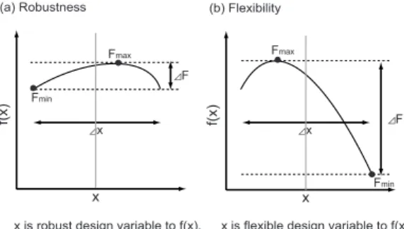
A. The concept of flexibility of design variable

Robust design that preserves the quality of the products is very important, and there has recently been a focus on flexibility design[15], [16], [17], [18], [19]. In flexibility design, some of the inner parameters can be changed dy- namically and the characteristics of the designs can be altered along with the changes in these parameters. These changes in the characteristics can be applied readily to changes in the environment and various needs of the user.

Products designed to maintain high flexibility can be applied not only to changes in the environment but also to the various needs of the user. In

2

<x < x+ x

2

, Robustness and Flexibility of the objective function,

are formulated as follows.

Robustness

is smaller.

Flexiblity

is larger. (3) If

is minimum,

lim

x!0 F

max F

min

=j F

j

Fig. 4. Concept of Robustness and Flexibility

Robustness

x

j

is smaller.

Flexiblity

x

j

is larger.

(4)

Where

and

are the maximum and minimum values of

respectively, and

F

min

.

in Robustness is unpredictable,

in Flexibility is predictable and adaptive.

The robustness and flexibility of the design variables are shown in Fig. 4.

When the products have high robustness in their design variables, small changes in the design variables do not affect the evaluation functions. These design methods have advantages in the case of errors in the design variables in the production process. On the other hand, changes in the design variables strongly affect the evaluation functions in flexible designs. These design methods are advantageous when the products require a wide range of evaluation functions. Here, we focus on flexibility.

Flexibility can be measured to find gaps in the evaluation function along with changes in the design variables. This is the flexibility of the design variables to a certain function.

In the next section, we discuss the flexibility of the design variables to the Pareto-optimal solutions in multi-objective optimization.

B. Flexibility in Multi-objective Optimization

The previous section described the flexibility of design variables. However, there is only one function in this expla- nation. In multi-objective optimization, as there are several evaluation functions, the conditions of flexibility are differ- ent.

Fig. 5 illustrates two types of the flexibility in multi- objective optimization.

In Fig. 5, the Pareto-optimal solutions are derived with several design variables. The dotted line indicates the Pareto- optimal solutions. Here, we changed the values of certain design variables with the remaining design variables fixed.

In Fig. 5(a), the values of the evaluation functions are

also changed. These changes are similar to the Pareto-

optimal solutions. The changes in the evaluation functions

are also illustrated in Fig. 4(b). In this case, the changes are

completely different from the Pareto-optimal solutions and

each change is dominated to the Pareto-optimal solutions.

Fig. 5. Two types of concept of Flexibility

Fig. 6. Robustness and Flexibility of design variables

In case(a), we can determine that the change in the focused parameters can cover the Pareto-optimal solutions even when the other design parameters are fixed. On the other hand, in case (b), the change in the focused parameters cannot cover the Pareto-optimal solutions at all.

From this discussion, we can define the flexibility of the design variables to the Pareto-optimal solutions as follows:

the focused design variables have high flexibility to Pareto- optimal solutions in case (a) but not in case (b).

When a certain design variable has flexibility to the Pareto- optimal solutions, then the Pareto-optimal solutions can be derived without this design variable. One of the goals of multi-objective optimization is to derive the Pareto-optimal solutions. Usually, when we use a wide variety of design vari- ables, we can derive a wider range of different Pareto-optimal solutions. However, from the discussion of the flexibility to the Pareto-optimal solutions, it can be concluded that some design parameters are not necessary to derive the Pareto- optimal solutions if these parameters do not have flexibility.

Therefore, it is very important to derive the flexibility to the Pareto-optimal solutions.

Here, we summarize the concept of robustness and flexi- bility to the Pareto-optimal solutions in Fig. 6.

In Fig. 6, there are three design parameters,

,

and

x

3

, which are used to derive the Pareto-optimal solutions. In this example, one of the design variables is changed and the others are fixed. The effects of the changes in each design variable on the evaluation functions are different. When

is changed, the change in

is large but that in

is small.

In the same manner, when

is changed, the change in

is large but that in

is small. On the other hand, the change in

x

3

does not affect the Pareto front. These results suggest that the robustness of

to the evaluation functions is very high.

x

1

has flexibility to

and

has flexibility to

. Therefore, the derived Pareto-optimal solutions may be derived only with

and

.

The decision making is one of the most difficult prob- lems in multi-objective problems. Designers always straggle to determine the final design parameters from the derived Pareto-optimal solutions. When there are many design pa- rameters and some of are not important for the Pareto-optimal solutions, it is very difficult to determine the final design parameters. For designers, it is much easier to find the final design parameters from a small number of design variables.

Products with a small number of design variables can be produced at low cost.

Therefore, the flexibility of design variables to the Pareto- optimal solutions is very important. In the following section, we illustrate measurement of the flexibility of design vari- ables to the Pareto-optimal solutions.

C. Evaluation Method of Flexibilities of Design Variables to Pareto-optimal Solutions

The previous sections described the importance of flex- ibility of design variables to the Pareto-optimal solutions.

However, it is very difficult to evaluate flexibility to the Pareto-optimal solutions. To find the flexibility of each design variable, the changes in the evaluation functions should be measured along with the changes in the focused parame- ter under conditions where the values of the other design variables are fixed. Of course, these fixed values affect the changes in the evaluation functions. Therefore, it is very important to determine these fixed values.

In this paper, we propose a method for evaluation of the flexibility of design variables to the Pareto-optimal solutions as follows (Fig. 7).

1) Formulate the multi-objective problem. This problem is solved using all the design variables. In this case, no design variable values are fixed.

2) The derived Pareto-optimal solutions are sorted along with the value of a certain object function.

3) Five points are determined from the sorted Pareto- optimal solutions. The distances between the five points should be the same.

4) In each point, one of the design variables is changed.

In this case, the values of the other solutions are fixed. The range of the design variable is assumed.

In this condition, the multi-objective optimization is performed again and the new Pareto-optimal solutions are derived. These new Pareto-optimal solutions de- termined along with the changes in the parameter are equal to the flexibilities of this point.

5) The flexibilities of all design variables and all five points are derived.

From this procedure, the flexibility of the design variable

to the Pareto-optimal solution is derived. In this procedure,

the values of the Pareto-optimal solution are used as fixed

Fig. 7. Method for measuring flexibility

Fig. 8. Pareto-optimal Solutions (SFC, NOx)

values. Among the steps, step 4 is very important. Since non- dominated solutions are derived again from the solutions with along to the change of one design variable, the results are totally different from the sensitinity analysis of the objective functions.

D. Examination of Method for Evaluation of Flexibilities of Design Variables

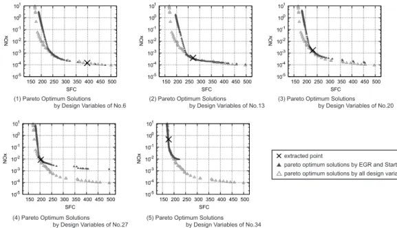
In the previous sections, the method for evaluation of flex- ibilities of design variables to the Pareto-optimal solutions was described. Examination of this method is discussed in this section. First, the results of the optimized diesel engine fuel emission scheduling problem without fixed design vari- ables are shown in Fig. 7. The diesel engine fuel emission scheduling problem has three objective functions, but we focused on only two-SFC and NOx, for ease of visually grasping the distribution of solutions.

The results of optimization with three objective functions are shown on the left of Fig. 8, and the results focusing on the Pareto-optimal solutions of NOx and SFC are shown on

the right of Fig. 8. Among the Pareto-optimal solutions (39 individuals) of NOx and SFC, five points were extracted.

These five were 6, 13, 20, 27, and 34th optimum solution sorted in ascending order according to NOx value. The design variable values of each extracted optimal solution are shown in Table. I.

Multi-objective optimization is performed by the design variable that measures flexibility, using the design variable values of each solution shown in Table. I as fixed values. The relationships between SFC of the optimized Pareto-optimal solutions and each design variable are shown in Fig. 9, and the relationships between NOx of the optimized Pareto- optimal solutions and each design variable are shown in Fig.

10.

The sub-figures((1)

(5)) in Fig. 9 show the results of optimizing with only the arbitrary design variables unfixed at each extraction point.

In Fig. 9-(3), the values of SFC change markedly when StartAngle is changed in all of the extracted points. There- fore, we can see that flexibility of StartAngle regarding SFC is high. Moreover, in Fig. 9-(1), as the values of SFC do not change when BoostPressure is changed in any of the extracted points, we can see that flexibility of BoostPressure regarding SFC is low and the robustness is high. In Fig.

10-(2), the values of NOx change markedly when EGR is changed in all of the extracted points. Therefore, we can see that flexibility of EGR regarding NOx is high. Moreover, in Fig. 10-(1), we can see that flexibility of BoostPressure regarding NOx is low and the robustness is high.

The above results indicate that using the proposed method it is possible to estimate the flexibility of the Pareto-optimal solutions. Moreover, we can also confirm that flexibility differs among the solutions chosen from the Pareto-optimal solutions, and not only flexibility but the robustness of a design variable can be confirmed.

The next section describes analysis regarding the useful- ness of using design variables with high flexibility to SFC and NOx when performing flexible design of the diesel engine fuel emission scheduling problem.

E. Examination of the Design Variable For a Flexible Design The design variables, StartAngle and EGR, have high flex- ibility regarding NOx and SFC and are used in optimization.

The optimized results are shown in Fig. 11.

From Fig. 11-(3), we can see that the Pareto-optimal solu- tions obtained are similar to those obtained when all design variables were unfixed. Moreover, other results indicated that various Pareto-optimal solutions were obtained.

The above results indicate that it is possible for a flexible design of a diesel engine, with StartAngle and EGR as the only unfixed design variables, to achieve similar performance compared to the case where all design variables are unfixed.

V. C ONCLUSIONS

The importance of flexible systems that can change their

characteristics along with the internal parameters has at-

tracted a great deal of attention. Flexible systems can adapt

TABLE I

D

V

E

P

Extracted Points SFC NOx BoostPressure EGR Duration Angle StartAngle

6 396.312 0.000137 3.50161 0.3 36 6.39216

13 270.225 0.000378 3.65 0.3 36 -3.80392

20 229.35 0.001679 3.57903 0.3 35.5 -4.11765

27 205.126 0.008548 3.59839 0.3 35.5 -4.66667

34 175.069 0.450112 3.65 0.241935 25 -9.68627

Fig. 9. Relations of SFC and Design Variables

Fig. 10. Relations of NOx and Design Variables

to changes in the environment and be applied to a wide variety user needs. To design flexible systems, these internal parameters should be determined. When there are several design parameters, multi-objective optimization problems are solved. In this case, one of the goals is to derive the Pareto- optimal solutions. The Pareto-optimal solutions are derived with several design variables. However, in some cases, some design variables do not contribute to the Pareto-optimal

solutions. As the flexibility of these variables is small, the

other variables can cover construction of the Pareto-optimal

solutions. Therefore, the flexibility of the design variables to

the optimum solution is very important. This paper illustrated

the concept of flexibility of the design variables to the

Pareto-optimal solutions. At the same time, the method for

evaluation of the flexibility of the design variables to the

optimum solutions was introduced. In the proposed method,

Fig. 11. Pareto-optimal Solutions (StartAngle, EGR)

one of the design variables is changed and the change in the Pareto-optimal solutions is evaluated under conditions where the rest of the design variables are fixed. In this case, the fixed values are very important. We propose deriving these values from the points of the Pareto-optimal solutions. In addition, we showed that the Pareto-optimal solutions can be derived only with the design variables whose flexibilities are high in the diesel engine fuel emission scheduling problem.

The following items remain for future studies:

In the proposed procedure, five points scattered on the Pareto-optimal solutions are used. Further discussion of the number of points, their location, etc., should be performed.

In this paper, only multi-objective optimization prob- lems with two objectives were discussed. In future work, we will propose an evaluation method for multi- objective optimization problems that have more than three objectives.

In our studies, we will introduce design systems for flexible systems.

R EFERENCES

[1] Kalyanmoy Deb. Multi-Objective Optimization using Evolutionary Algorithms. Chichester, UK : Wiley, 2001.

[2] D. E. Goldberg. Genetic Algorithms in search, optimization and machine learning. Addison-Wesly, 1989.

[3] C. M. Fonseca and P. J. Fleming. Genetic algorithms for multiob- jective optimization: Formulation, discussion and generalization. In Proceedings of the 5th international coference on genetic algorithms, pages 416–423, 1993.

[4] E. Zitzler and L. Thiele. Multiobjective evolutionary algorithms:

A comparative case study and the strength pareto approach. IEEE Transactions on Evolutionary Computation, 3(4):257–271, 1999.

[5] Alex Mayer Mark Erickson and Jeffrey Horn. The niched pareto genetic algorithm 2 applied to the design of groundwater remediation systems. In In Eckart Zitzler, Kalyanmoy Deb, Lothar Thiele, Carlos A. Coello Coello, and David Corne, editors, First International Con- ference on Evolutionary Multi-Criterion Optimization,Springer-Verlag.

Lecture Notes in Computer Science No. 1993, pages 681–695, 2000.

[6] Amrit Pratab Kalyanmoy Deb, Samir Agrawal and T. Meyarivan. A fast elitist non-dominated sorting genetic algorithm for multi-objective optimization: Nsga-ii. In KanGAL report 200001, Indian Institute of Technology, Kanpur, India, 2000.

[7] E. Zitzler, M. Laumanns, and L. Thiele. Spea2: Improving the per- formance of the strength pareto evolutionary algorithm. In Technical Report 103, Computer Engineering and Communication Networks Lab (TIK), Swiss Federal Institute of Technology (ETH) Zurich, 2001.

[8] H. Hiroyasu and T. Kadota. Models for Combustion and Formation of Nitric Oxide and Soot in Direct Injection Diesel Engines. SAE Paper 760129, 1976.

[9] Hiroyuki HIROYASU, Toshikazu KADOTA, and Masataka ARAI. De- velopment and Use of a Spray Combustion Modeling to Predict Diesel Engine Efficiency and Pollutant Emissions (Part 2 Computational Procedure and Parametric Study). Bulletin of the JSME, 26(214):576–

583, April 1983.

[10] T. W. Kuo. Evaluation of a Phenomenological Spray-Combustion Model for Two Open-Chamber Diesel Engines. SAE Paper 872057, 1987.

[11] K. Nishida and H. Hiroyasu. Simplified Three-Dimensional Modeling of Mixture Formation and Combusion in a d.i. Diesel Engine. SAE Paper 890269, 1989.

[12] K. Yoshizaki. T.Ishida and H. Hiroyasu. Approach to Low nox and smoke Emission Engines by Using Phenomenological Simulation. SAE Paper 930612, 1993.

[13] T Imanishi, H. Yoshizaki and H. Hiroyasu. Simulation Study of Effects of Injection Rate Profile and Air Entrainment Characteristics on d.i.

Diesel Engine. SAE Paper 962059, 1996.

[14] Gakumazawa H. Long, Y. S. and H. Hiroyasu. The Simulation of the Distribution of Temprature and Mass of Liquid and Vapor Fuels, and the Wall Impinging Spray Pattern in a Diesel Combustion Chamber.

SAE Paper 2000-01-1887, 2000.

[15] Nair A. R. Bloebaum C. L. English, K. and Lewis. Layout opti- mization for component packing. In 2nd International Conference on Engineering Design and Automation, Maui, HI, 1998.

[16] J. Root. Aerospace technology development: X-33 shield takes the heat,. In Aerospace Technology Innovation, 6(4),July/August 1998.

[17] C. D. Jilla and D. W. Miller. Satellite design: Past, present and future,.

In International Journal of Small Satellite Engineering, 8,July 1997.

[18] M. Janah. Changing gears,. In Red Herring, pages 230–232, August 2000.

[19] A. Webb. A piston revolution,. In Engineering Management Journal,

pages 25–30, February 2002.