A Proposal of Spatio-Temporal Reconstruction Method Based on a Fast Block-Iterative Algorithm

(1)

PAPER

Special Section on Medical Imaging

A Proposal of Spatio-Temporal Reconstruction Method Based on a Fast Block-Iterative Algorithm

Tatsuya KON^†a),Student Member, Takashi OBI^†,Member, Hideaki TASHIMA^††,Nonmember, andNagaaki OHYAMA^†,Member

SUMMARY Parametric images can help investigate disease mecha- nisms and vital functions. To estimate parametric images, it is necessary to obtain the tissue time activity curves (tTACs), which express temporal changes of tracer activity in human tissue. In general, the tTACs are calculated from each voxel’s value of the time sequential PET images estimated from dynamic PET data. Recently, spatio-temporal PET reconstruction methods have been proposed in order to take into account the temporal correlation within each tTAC. Such spatio-temporal algorithms are generally quite computationally intensive. On the other hand, typical algorithms such as the preconditioned conjugate gradient (PCG) method still does not provide good accuracy in estimation. To overcome these prob- lems, we propose a new spatio-temporal reconstruction method based on the dynamic row-action maximum-likelihood algorithm (DRAMA). As the original algorithm does, the proposed method takes into account the noise propagation, but it achieves much faster convergence. Performance of the method is evaluated with digital phantom simulations and it is shown that the proposed method requires only a few reconstruction processes, thereby remarkably reducing the computational cost required to estimate the tTACs.

The results also show that the tTACs and parametric images from the proposed method have better accuracy.

key words: PET, parametric image, spatio-temporal reconstruction, DRAMA

1. Introduction

Dynamic data from positron emission tomography (PET) can provide parametric images, which can be used to vi- sualize important physiological and biochemical information. Such information can help elucidate disease mecha- nisms or vital functions in the human or animal body. Here we outline the general steps that must be taken to estimate parameter values of the image. First, emission images are reconstructed from PET data with respect to each time frame. From the image sequence we can determine tissue time activity curves (tTACs), which express the temporal change of tracer activity at each voxel. Parameters may be obtained from the tTACs and plasma time activity curve (pTAC) by fitting a kinetic model, such as two-tissue three- compartment model shown in Fig. 1. Methods are available for both linear (e.g. Patlak graphic plot [1]) and non-linear (e.g. modified Marquardt approach [2]) compartment model analysis.

Manuscript received June 26, 2012.

Manuscript revised October 26, 2012.

†The authors are with the Tokyo Institute of Technology, Yokohama-shi, 226–8503 Japan.

††The author is with the National Institute of Padiological Sci- ences, Chiba-shi, 263–8555 Japan.

a) E-mail: [email protected] DOI: 10.1587/transinf.E96.D.819

Since pTAC can be measured e.g., from arterial blood sampling with high accuracy, the parametric image quality is strongly dependent on the accuracy of tTAC estimation.

The conventional approach, however, produces noisy images since typical reconstruction algorithms neglect information from neighboring frames.

To reduce the noise, there have been proposals of some spatio-temporal reconstruction methods with temporal basis function that take into account the temporal correlation within each tTAC [3], [4]. Alternatively, some reconstruction methods estimate the parameters directly from the pro- jection data, which could involve the data from all dynamic frames in the reconstruction [5].

In line with the former studies, we might consider a spatio-temporal reconstruction to maximize a cost function derived from statistical properties. Such algorithms, however, have remarkably high computational cost.

Meanwhile, in the spatial reconstruction field, block- iterative algorithms have been developed, including row- action maximum likelihood algorithm (RAMLA) [6] and dynamic RAMLA (DRAMA) [7], [8], proposed to improve the convergence of maximum likelihood estimation. In par- ticular, it was reported that DRAMA provided reasonable signal-to-noise ratio with a satisfactory spatial resolution using only a few iterations.

This paper presents a new spatio-temporal reconstruction method based on DRAMA for list-mode data to estimate tTACs with a high voxel-by-voxel accuracy and also reducing computational cost. The proposed method allows for fast while properly adjusting noise propagation. We evaluate performance of this method with a digital phantom simulation. The proposed method remarkably reduces the

Fig. 1 Three-compartment model. The parametersK1,k2,k3, andk4

denote the transfer rate between compartments.k4is negligible for e.g., the

18F-FDG model.

Copyright c2013 The Institute of Electronics, Information and Communication Engineers

(2)

computational time required to estimate the tTACs. Also, the tTACs and parametric images estimated using the proposed method show good performance in terms of voxel- by-voxel estimation.

2. Method

We assume in this paper that dynamic PET data set has been given as a list-mode format, which has the detection information stored event by event. We express the PET measurement data, includingNnumber of events, as

S ={(in,tn)|1≤n<N}, (1) where then-th event has been detected at a detector pair of indexinat the sampled time of indextn. Next we formulate the relation between the list-mode data set denoted byS and tTAC, which is needed to make parametric images. Let jbe the voxel index in object space,xj(t) be the tTAC at the j-th voxel, andai j be a detection sensitivity that events emitted fromj-th voxel are caught byi-th detector pair. Since events are detected according to Poisson distribution, the probability that the event detected at detector pairinand at timetn, given{xj(t)}, would be

Pr(in,tn| {xj(t)})=exp

⎛⎜⎜⎜⎜⎜

⎜⎝−

j

ai_njxj(t)

⎞⎟⎟⎟⎟⎟

⎟⎠

⎛⎜⎜⎜⎜⎜

⎜⎝

j

ai_njxj(t)

⎞⎟⎟⎟⎟⎟

⎟⎠. (2) Here we adopt a basis function set for tTACs, which was introduced in [3]:

xj(t)=

lmax

l=1

wjlBl(t), (3)

wherewjldenotes thel-th coeﬃcient at voxel jandBl(t) denotes thelmaxnumber of basis functions. In general, smooth basis functions are preferred since the tTACs tend to be tem- porally correlated. For example, a set of B-spline basis functions is often chosen because of their easy implementation and of the locality of each basis curve. Alternatively, we could choose a set of functions that would well repre- sent the curves generated from a specific radioactive tracer.

This could be feasible if we know the characteristics of the curves.

The probability of the measurement ofS, given xj(t), is derived from Eq. (2) and Eq. (3) as

Pr(S | {xj(t)}) =

n∈S

Pr(in,tn| {xj(t)})

=

n∈S

exp

⎛⎜⎜⎜⎜⎜

⎜⎝−

j

ai_nj

l

wjlBl(t)

⎞⎟⎟⎟⎟⎟

⎟⎠·

⎛⎜⎜⎜⎜⎜

⎜⎝

j

ai_nj

l

wjlBl(t)

⎞⎟⎟⎟⎟⎟

⎟⎠, (4) and thus we obtain the log-likelihood function

L(w) =log⎧⎪⎪⎪⎨

⎪⎪⎪⎩

n∈S

j

ainj

l

wjlBl(tn)⎫⎪⎪⎪⎬

⎪⎪⎪⎭

−

i

j

ai j

l

wjl

T 0

Bl(t)dt, (5) wherewdenotes a vector containingwjlfor all j=1, . . . ,J andl = 1, . . . ,lmax, andT denotes the measurement time.

Substituting the optimalwmaximizing Eq. (5) into Eq. (3), we can determine the tTACs, motivating our attempt to find the optimal w. Although we regard the simple log- likelihood function as the cost function in this paper, this approach could be easily extended by including a penalty function in Eq. (5), resulting in a penalized log-likelihood. Con- ventionally, expectation-maximization (EM) algorithm [4]

or preconditioned conjugate gradient (PCG) algorithm [3]

have been applied to obtain thewthat maximizes the cost function. These algorithms, however, require a large number of iterations before convergence.

To speed up convergence, we adopt an approach based on DRAMA [7], [8], a block-iterative algorithm. DRAMA was developed as a spatial reconstruction algorithm and has been reported to improve the convergence of maximum likelihood estimation. DRAMA has the characteristic definition of a relaxation parameter as described below. Here we can apply a similar approach as the derivation of the block-iterative algorithms for list-mode data [8]. To intro- duce the block-iterative method to maximize the cost function Eq. (5), we decompose it into a summation ofMpartial cost functionsLm(w), i.e.,

L(w)=

M−1 m=0

Lm(w). (6)

Also, we divide the list-mode data set into subsetsSm(m= 0, . . . ,M−1).

To define the partial cost function that satisfies Eq. (6), we adopt ablocking-factor pm j, which is introduced in [8]

to determine how to decompose the log-likelihood function.

In this paper, define this as pm j=

iai j

M−1 m=0

n∈Smainj

=

iai j

n∈Sai_nj, (7)

which satisfies

m

n∈S_m pm jai_nj =

iai j. Then we may define the partial cost function as

Lm(w) = log

⎛⎜⎜⎜⎜⎜

⎜⎝

n∈Sm

j

ai_nj

l

wjlBl(tn)

⎞⎟⎟⎟⎟⎟

⎟⎠

−

j

pm jai j

l

wjl

T 0

Bl(t)dt, (8) each of which involves just the corresponding subsetSm. Applying the idea of block-iterative method with the deriva- tive ofLm(w), we derive a new iterative algorithm as fol- lows:

(3)

w^(k_jl^,⁰⁾=w^(k)_jl, (9) w^(k_jl^,^m⁺¹⁾=w^(k_jl^,^m)+λ^(k^,^m)w^(k_jl^,^m)

Cjl

n∈S_m

ai_nj·

⎛⎜⎜⎜⎜⎜

⎜⎝ Bl(tn)

jainj

lw^(k_jl^,^m)Bl(tn)−pm j

T 0

Bl(t)dt

⎞⎟⎟⎟⎟⎟

⎟⎠, (10)

w^(k_jl⁺¹⁾=w^(k_jl^,^M), (11)

and

Cjl=max

m

n∈S_m

pm jai_nj

T 0

Bl(t)dt, (12) for all j =1. . .J,l =1. . .lmax,m =0. . .M −1, andk = 0,1, . . ., wherekis an index of current iteration andCjl is a normalization coeﬃcient. The variable λ^(k^,^m) appearing in Eq. (10) is a relaxation parameter for providing uniform noise propagation [7]. One possibility for this is

λ^(k^,^m) = β0

β0+m+γkM, (13)

whereβ0is a constant dependent on a geometrical correlation function andγis a constant value determined empiri- cally.

In the proposed algorithm, it is necessary to random- ize the observed list-mode data before dividing them into subsets so that each subset has the same temporal information. If the list-mode data in each subset were to have un- equal temporal information, the proposed algorithm might not work correctly.

3. Simulation

We carried out a computer simulation to evaluate the performance of the proposed method and to investigate the quality of resulting images as compared with those resulting from conventional methods. This simulation was performed on data from a 3D PET scan, which has a huge number of measurement events compared with 2D scan and en- larges the problem of the computational cost [9], and on data from a¹⁸F-FDG brain phantom study for imaging cerebral metabolic rates, a typical PET tracer study [10]. We created a list-mode data set from a 3D PET measurement of a digital cylindrical phantom shown in Fig. 2.

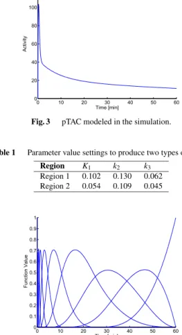
The phantom had hot regions whose diameters were 3.0 cm, 4.0 cm, and 4.5 cm respectively. Two regions of interest (ROIs), placed at the central slice and including 172 voxels, were set for the following evaluations (Fig. 2). The diameter of the field of view was set as 25.0 cm so that it could hold the whole phantom, and the field of view con- sisted of five slices. The image resolution of each slice was 100×100 voxels. Each voxel of the phantom had a tTAC that was one of the two types of tTACs according to the three- compartment model (Fig. 1). The pTAC for the input function was modeled as [11] (Fig. 3) and parameter values were set as in Table 1, which simulated¹⁸F-FDG studies.

Fig. 2 Digital phantom settings. ROIs were placed on the central slices of the phantom for evaluation.

Fig. 3 pTAC modeled in the simulation.

Table 1 Parameter value settings to produce two types of tTACs.

Region K1 k2 k3

Region 1 0.102 0.130 0.062 Region 2 0.054 0.109 0.045

Fig. 4 The basis function set used in the reconstruction processes in the simulation.

To begin with, we produced sinograms of the phantom at each second. We included background activity that amounted to 1/5 of all counts and added Poisson noise to the sinograms. Then we transformed them into list-mode format. The quantity of the list-mode count was approximately 5.0×10⁶counts and the noise level was 31.5 percent.

In the reconstruction process, we estimated tTACs from the list-mode data using the proposed method and also using two conventional spatio-temporal methods: the PCG method and the EM method. We adopted as the basis function model a set of 10 B-spline basis functions shown in Fig. 4, which we confirmed can express tTACs generated from the model. After we obtained the curves, we performed post-smoothing using a spatial Gaussian filter having a full

(4)

width at half maximum (FWHM) of two voxels. In the proposed method, we randomized the list-mode data and then divided them intoM = 100 subsets so that all the subsets had approximately the same counts. The constant valueβ0

andγwere defined as 51.6 and 0.1, respectively. In the PCG method, to avoid negative value estimates, we overwrote the values of the estimatewjl :=max(wjl,0) at the end of each iteration. For evaluation of the methods, we chose the iteration number at which we minimized the mean square error values between estimated curves within the ROI II and ideal curves, indicating the convergence of the estimates.

From the estimated tTACs, we generated parametric images by means of Patlak graphic plot analysis [1]. This analysis can produce parameter images of FDG-influx val- uesKi=K1k3/(k2+k3) by taking the slope of the integral of Cp(t) divided byCp(t) versusC(t)/Cp(t), whereCp(t) is the input function andC(t) is the time change of the voxel value.

The analysis processes were performed the same way for tTACs reconstructed with each of the three diﬀerent methods.

All calculation processes were performed on an Intel Xeon processer (2.93 GHz), and the processes of reconstruction were implemented for 8 core 16 thread parallel compu- tations by OpenMP.

4. Results

We recorded the voxel average of root mean square error (RMSE) values in ROI II between the reconstructed curves and the ideal curves. We defined the RMSE here as

RMSE= 1 JROI

j∈ROI

T

0

(x^(k)_j (t)−x^ideal_j (t))²dt, (14) whereJROIdenotes the number of voxels in the ROI.

Figure 5 depicts the RMSE values through 30 iterations of the methods. The RMSE value was smallest at one iteration of the proposed method, at 15 iterations of the PCG

Fig. 5 RMSE between tTACs and the ideal curve in ROI II through 30 iterations. The red line with the cross mark indicates the proposed method, the blue line with the plus mark indicates the PCG method, and the green line with the triangle mark indicates the EM method.

method, and at 25 iterations of the EM method. Computa- tional times for those iterations are shown in Table 2. The proposed method was more than 11 times faster than the

Table 2 Computational time for the three spatio-temporal reconstruction methods.

Method Time

DRAMA 1-iter 53 min PCG 15-iter 11 h 33 min EM 25-iter 13 h 42 min

Fig. 6 Estimated tTACs in ROI I. The curves were reconstructed with the proposed method (top), with PCG method (middle), and with EM method (bottom). The black dashed lines indicate ideal curves, the gray solid lines indicate several examples of tTACs, and blue solid lines indicate the mean values and the SD values within the ROI.

(5)

Fig. 7 Estimated tTACs in ROI II. The curves were reconstructed with the proposed method (top), with PCG method (middle), and with EM method (bottom). The black dash lines indicate ideal curves, the gray solid lines indicate several examples of tTACs, and blue solid lines indicate the mean values and the SD values within the ROI.

PCG method and more than 13 times faster than the EM method.

The tTACs estimated by all three methods for voxels in ROI I and in ROI II are shown in Fig. 6 and Fig. 7 respectively. In both figures, black dashed lines denote ideal curves, gray solid lines denote several examples of tTACs in the ROI, and blue solid lines denote the mean values and the standard deviation values of the tTACs within the ROI.

Figure 8 depicts the central slices of the parametric im-

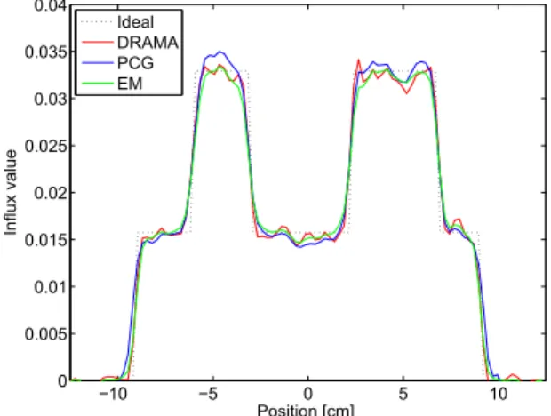
Fig. 8 Result parametric images at central slices. The line drawn on the ideal image is the profile line of Fig. 9.

Fig. 9 Line profile of the parametric images.

ages of FDG-influx values. The images were estimated from tTACs reconstructed with the three methods. Table 3 shows the numerical results of the two ROIs. The image produced from the proposed method had lower variance than that of the PCG method and lower bias than that of the EM method.

Figure 9 shows the horizontal profiles of the line drawn on the ideal image in Fig. 8.

5. Discussion

The reconstructed tTACs in Fig. 6 and Fig. 7 indicate that the proposed method achieved good convergence with just one iteration. In Fig. 6, the mean curves in ROI I using the proposed method would converge to the ideal curve while those using the PCG method would overestimate the curves, and those using the EM method would slightly underestimate during the latter half of the measurement time. It would seem in Fig. 7 that their variances of the curves have slight diﬀerence in the ROI.

In terms of the computational time shown in Table 2, the proposed method would achieves a faster convergence than conventional one. The dominant part of the algorithm is a loop calculation for each list-mode eventn. The time of this calculation of both proposed method and EM method would be almost the same order, and that of the

(6)

Table 3 Bias and stantard deviation (SD) of parameter values in ROIs.

Method DRAMA PCG EM

Bias [%]

ROI I −1.71 −0.13 −2.77 ROI II −0.19 −0.48 −0.74 SD [10⁻³]

ROI I 1.05 1.08 1.03 ROI II 0.249 0.247 0.246

PCG method would be longer. Note that only the proposed method has a non-negligible pre-calculation process to cal- culate the blocking factor values, which took 20 minutes in this simulation.

Figure 8 compares the parametric images from the tTACs reconstructed with three methods. We plot the horizontal profile (Fig. 9) along the line on the ideal image to see the diﬀerence among the parametric images. The image from tTACs obtained with the EM method might look blurred compared with other two estimated images. As shown in Fig. 9, a profile line of the image through the EM method process could express the value of the centers of hot regions; however, the profile would be slightly dull near the edge of the regions. The profile through PCG method would have similar values near the edge of the regions, while this would overestimate at the centers of hot regions. As a result, the PCG method had a quite low bias error in Table 3. Com- pared with the two, the profile through the proposed method could express the value around the edge of the regions. It could indicate that the proposed method has good performance in terms of voxel-by-voxel estimation. The proposed method achieved low bias especially in ROI II, with similar SD values as the other methods.

A limitation of the proposed method is that we still have to determine empirical settings. In the definition of the relaxation parameter, the geometrical correlation was derived by assuming a two-dimensional model [7], which was also used for three-dimensional reconstructions, or an actual three-dimensional model (here we adopted the former ver- sion). We might further improve estimation by a suitable definition for a four-dimensional model. In addition, we might have to determine the optimal number of subsets. In the proposed method, the amount of radioactivity could af- fect the signal to noise ratio of both spatio-temporal images and final parametric images compared with conventional algorithms. That is, if the number of subsets is redundant, each subset could have noisy data in remarkably low activity case, and it might invoke lower quality results.

Additionally, the choice of the number of basis functions could aﬀect the quality of resulting images both using the proposed algorithm and using conventional spatio- temporal algorithms. For instance, the reconstruction might require more basis functions to maintain suﬃcient time resolution of the curves.

Although we evaluated using only computer simulation, real PET data should be applied to validate a performance of the proposed method, which we leave for future work. Still, we would hope it would provide further va-

lidity of the proposed method. In such clinical PET mea- surements, photon scatter and signal attenuation may aﬀect results, factors we did not consider in our simulation. There are studies where attenuation and scatter models have been included in the system matrix [12]. These factors can be in- corporated by modifying the system matrix in the algorithm.

6. Conclusion

We developed a new method that extended a block-iterative algorithm called DRAMA for spatio-temporal reconstruction. We derived the method and evaluated it using a computer simulation. The results indicate that the proposed method has good performance for generating tTACs in terms of voxel-by-voxel estimation, and it requires considerably less computational time compared with conventional spatio- temporal methods. Although we focused in this paper on a simple maximum likelihood reconstruction, it can be extended to a penalized likelihood estimation by modifying the cost function.

References

[1] C.S. Patlak and R.G. Blasberg, “Graphical evaluation of blood-to- brain transfer constants from multiple-time uptake data. Generaliza- tions,” J. Cerebral Blood Flow and Metabolism, vol.5, no.4, pp.584–

590, Dec. 1985.

[2] D.W. Marquardt, “An algorithm of least square estimation of nonlin- ear prameters,” J. Society for Industrial and Applied Mathematics, vol.11, no.2, pp.431–441, June 1963.

[3] T.E. Nichols, J. Qi, E. Asma, and R.M. Leahy, “Spatiotemporal reconstruction of list-mode PET data,” IEEE Trans. Med. Imaging, vol.21, no.4, pp.396–404, April 2002.

[4] A.J. Reader and F.C. Sureau, C. Comtat, R. Tr´ebossen, and I. Buvat,

“Joint estimation of dynamic PET images and temporal basis functions using fully 4D ML-EM,” Physics in Medicine and Biology, vol.51, no.21, pp.5455–5474, Nov. 2006.

[5] M.E. Kamasak, C.A. Bouman, E.D. Morris, and K. Sauer, “Direct reconstruction of kinetic parameter images from dynamic PET data,”

IEEE Trans. Med. Imaging, vol.24, no.5, pp.636–650, May 2005.

[6] J. Browne and A.B. de Pierro, “A row-action alternative to the EM algorithm for maximizing likelihood in emission tomography,” IEEE Trans. Med. Imaging, vol.15, no.5, pp.687–699, Oct. 1996.

[7] E. Tanaka and H. Kudo, “Subset-dependent relaxation in block- iterative algorithms for image reconstruction in emission tomography,” Physics in Medicine and Biology, vol.48, no.10, pp.1405–

1422, May 2003.

[8] T. Nakayama and H. Kudo, “Derivation and implementation of ordered-subsets algorithms for listmode PET data,” IEEE Nu- clear Science Symposium and Medical Imaging Conference Conf., no.M5-7, Oct. 2005.

[9] T. Yamaya, E. Yoshida, T. Obi, H. Ito, K. Yoshikawa, and H.

Murayama, “First human brain imaging by the jPET-D4 prototype with a pre-computed system matrix,” IEEE Trans. Nucl. Sci., vol.55, no.5, pp.2482–2492, Oct. 2008.

[10] D.H.S. Silverman, “Brain 18F-FDG PET in the diagnosis of neu- rodegenerative dementias: comparison with perfusion SPECT and with clinical evaluations lacking nuclear imaging,” J. Nuclear Medicine, vol.45, no.4, pp.594–607, April 2004.

[11] D. Feng, D. Ho, K. Chen, L.C. Wu, J.K. Wang, R.S. Liu, and S.H.

Yeh, “An evaluation of the algorithms for determining local cerebral metabolic rates of glucose using positron emission tomography dynamic data,” IEEE Trans. Med. Imaging, vol.14, no.4, pp.697–710,

(7)

Dec. 1995.

[12] M. Tamal, A.J. Reader, P.J. Markiewicz, P.J. Julyan, and D.L.

Hastings, “Noise properties of four strategies for incorporation of scatter and attenuation information in PET reconstruction using the EM-ML algorithm,” IEEE Trans. Nucl. Sci., vol.53, no.5, pp.2778–

2786, Oct. 2006.

Tatsuya Kon received a B.E. degree in computer science from Tokyo Institute of Tech- nology, Tokyo, Japan, in 2009. He received an M.E. degree in information processing from To- kyo Institute of Technology, Tokyo, Japan, in 2011. He is currently a Ph.D. student in information processing at Tokyo Institute of Technol- ogy.

Takashi Obi received M.E. and Ph.D. degrees in information processing from Tokyo In- stitute of Technology, Tokyo, Japan, in 1992 and 1997, respectively. He was a Research Asso- ciate (1995–2002) at Imaging Science and Engi- neering Lab., Tokyo Institute of Technology and a Visiting Researcher (1998, 2000) at Univ. of Pennsylvania. He has been an Associate Profes- sor at Tokyo Institute of Technology since 2002.

His current interests include medical imaging, system security management and health infor- matics.

Hideaki Tashima received B.E., M.E., and Ph.D. degrees from Tokyo Institute of Technol- ogy in 2004, 2006, and 2009, respectively. Dur- ing 2009 and 2010, he was a postdoctoral researcher at the Imaging Science and Engineer- ing Laboratory, Tokyo Institute of Technology.

During 2011 and 2012, he was a postdoctoral fellow at the National Institute of Radiological Sciences (NIRS), Chiba Japan. He is currently a postdoctoral research fellow of the Japan society for the promotion of science (JSPS) at the NIRS.

Nagaaki Ohyama received a Ph.D. degree in information processing from Tokyo Institute of Technology, Tokyo, Japan, in 1982. He was a Research Associate (1983–1988) and an As- sociate Professor (1988–1993) at Imaging Sci- ence and Engineering Lab., Tokyo Institute of Technology and a Visiting Researcher (1986–

1989) at Univ. of Arizona. He has been a Profes- sor at Tokyo Institute of Technology since 1993.

His current interest includes medical imaging, e-government and procurement systems.