光円錐ハミルトニアンにおけるくりこみ群の方法

光円錐ハミルトニアンにおけるくりこみ群の方法

杉原, 崇憲

九州大学理学研究科物理学専攻

https://doi.org/10.11501/3122894

出版情報：Kyushu University, 1996, 博士（理学）, 課程博士 バージョン：

Department of Physics, Kyushu University, Fukuoka 812, Japan (

December

26, 1996)

Abstract

A perturbative renormalization group

(RG)

scheme for the light-front Hamil­

tonian is formulated on the basis of the Bloch-Horowitz effective Hamiltonian, and applied to the simplest

q}

model with spontaneous symmetry breaking of Z2 symmetry.

RG

equations are derived at one-loop order for both symmet­

ric and broken phases. The equations are consistent with those calculated in the covariant perturbation theory. For the symmetric phase, an initial cut­

off Hamiltonian in the

RG

procedure is defined by excluding the zero-mode from the canonical Hamiltonian with an appropriate regularization. An ini­

tial cutoff Hamiltonian for the broken phase is constructed by shifting a field

¢(

x

)

by

¢(

x

)

=

'P(

x

)

+ v in the initial Hamiltonian for the symmetric phase.

The vacuum expectation value v is determined as a function of the original running parameters so that the relation does not depend on the unphysical cutoff parameter. On the basis of the perturbative considerations, the three­

dimensional real scalar model is renormalized in a nonperturbative manner on a truncated Fock space. A critical line is calculated by diagonalizing the Hamiltonian regularized with basis functions. The marginal

( ¢6)

coupling dependence of the critical line is weak. The vacuum expectation value v is determined as a function of running mass and coupling so that the mass of the ground state vanishes.

the quantum chromodynamics

(

^QCD

)

nonperturbatively to investigate low-en rgy hadronic physics. The most reasonable nonperturbative method for u h a problem is th latti e gauge theory. In the method, it is easy to calculate the lightest particle state, but not to evaluate the excited and scattering states. Although there exist many nonperturbative prescriptions in the Hamiltonian formalism, the formalism has been abandoned so far sin Lorentz invariance and the renormalizability are not obvious.

The light-front

(

^LF

)

^Tamm-Dancoff field theory

[1]

is known as a m thod bas d on the Hamiltonian formalism. The Hamiltonian is constructed by quantizing fields on the light-front and truncating the Fock space. The truncation is called the Tamm-Dancoff ap­

proximation

[2].

The completeness of the Fock space is approximated ^as

���p In) (nl

^rv

1,

where NTD ----t oo corresponds to the full theory. It is possible to calculate mass spectra nonperturbatively by diagonalizing the Hamiltonian in the space. The resulting mass spec­

trum seems to be accurate for low-lying states, since the pair creation and annihilation are suppressed in the LF field theory, especially the pair creation of particles from the LF vac­

uum is kinematically prohibited. The prohibition warrants the truncation to be reliable.

This is really true in two-dimensional gauge theories

[3-5],

since the physical vacuum is trivial in the light-front field theory

[6-9]

and as the natural result the states have simple structures. This is an advantage of this method, but, at the same time, it causes a problem.

No pair creation means that the vacuum is trivial

HIO)

⁼

0,

i.e., the vacuum is always symmetric and can not posses information of the symmetry in the LF field theory. This is a serious problem, because various phenomena are explained as results of spontaneous

symmetry breaking

(SSB)

in the relativistic field theory. How can the LF field theory de­

scribe

SSB?

It has been said that the zero-mode operator leads the LF field theory to

SSB

[6,10].

We have a constraint equation for the zero-mode, if the system is quantized in a box

works

[7-9]

for the two-dimensional real scalar model, in which the zero-mod con traint equation is solved under reasonable approximations to describe SSB of the Z2 symm try. At least for the two-dimensional case, the light-front formulation seems to be consist nt with the equal-time one, if the zero-mode contributions are treated properly. Thi approa h to SSB has never been applied to higher dimensional models having ultraviolet div rg nc .

The main purpose of this paper is to propose practical perturbative and nonp rturbative RG schemes and describe SSB by using the schemes. The light-front field th ory raises complicated renormalization issues, when it is applied to realistic higher dimensional field theories, because of the non-covariant Hamiltonian formulation. As a powerful method for solving such renormalization issues in light-front field theory, we consider Wilson's renor­

malization group

(

^RG

)

^approach

[13],

in which renormalization is achieved automatically by finding a fixed point and a renormalization trajectory. Perry

[12]

applies the Minkowski­

space version of Wilson's RG approach

[14]

for the light-front Hamiltonian. Glazek and Wilson formulate a new perturbative RG scheme for the Hamiltonian by using a sp cially designed similarity transformation

[15].

The two RG schemes are based on perturbation and reliable for an analysis of RG flows near a Gaussian fixed point. In this paper, Bloch­

Horowitz effective Hamiltonian

[16]

is used here in order to achieve renormalization. This scheme is applied to the simplest

¢4

model in four dimensions. Our RG scheme is sim­

ple compared with the other two, since it contains no nonlinear equation. This scheme is, furthermore, free from the "vanishing energy denominator" problem, as shown in Sec. II.

This scheme was originally introduced by Perry in the context of light-front field theory, but not accepted because of the energy dependence of the effective Hamiltonian

[12].

^The

dependence means that the effective Hamiltonian is not Hermitian, but it does not cause problems in practice, as shown in Sec. II. The resultant RG equations are energy indepen-

the correct vacuum expectation value

(VEV)

to restore positivity of the spectrum. As a result, we have an asymmetric Hamiltonian HA, in which the RG parameter spa i larger than that for the symmetric Hamiltonian Hs. This is equivalent to assuming that th asymmetric Hamiltonian originally includes symmetry breaking interactions. There hould exist a relation among

VEV

and running parameters which does not depend on an unphy ical cutoff parameter. The

VEV

is determined from the relation as a function of th original parameters. The broken phase is an RG invariant surface containing the critical line in the parameter space of the asymmetric theory. The symmetry breaking interactions were originally introduced by Perry and Wilson in the coupling coherence study

[19,12],

_{but the}

instability of the canonical Hamiltonian was not mentioned.

The considerations mentioned above strongly depend on perturbation. In order to inves­

tigate the instability of the canonical Hamiltonian Hs in the broken phase, we renormalize the real scalar model in three dimensions with a nonperturbative RG prescription based on the Tamm-Dancoff truncation. The theory is regularized by expanding wavefunctions in terms of basis functions in a truncated momentum space. The mass spectrum is then obtained by diagonalizing the Hamiltonian within a space spanned by the basis functions.

In actual calculations we take the Fock space up to three-body states. The truncation is justified by examining the wave functions. The marginal coupling dependence of the critical line is also analyzed. A proper Hamiltonian for the broken phase is construct d by shifting the field as

¢(x)

=

<p(x)

_{+ v.} A relation of v to the original parameters are nonpertur­

batively determined by searching the critical surface which gives a vanishing mass for the ground state.

The paper is organized as follows. Section II presents our RG scheme. In Sec. III, the scheme is applied to

¢4

_{model in 3 +}

1

dimensions with spontaneous symmetry breaking

on basis functions is introduced. In Sec IV C, numerical RG is carried out by u ing the nonperturbative regularization mentioned above. Section V is devoted to summary and discussions.

Notational conventions are summarized as x± =

(x0

^{± xd-1}

)/.J2

^{, time x+, space}

(

^{x-, x..L}

)

^{, momentum}

k

⁼

(

^k+,

k..L),

^{metric g+-= g+- = -gii = -gii = l}

(

^{i =} 1, ... , d- 2

)

and others= 0, and LF energy k-=

E(k)

⁼

(ki

^{+ r}

)/

2k+, where r is a mass parameter.

II. PERTURBATIVE RG SCHEME

The basic RG procedure for the Hamiltonian is the following.

(

^l

)

A bare Hamiltonian is regularized by truncating Fock space at a large cutoff energy

A0.

The regularized Hamiltonian

HAo

is regarded as the initial Hamiltonian in RG procedure.

(

²

)

The truncated space is separated into the lower- and higher-energy sectors. An effective Hamiltonian

HA

for the lower-energy sector is constructed in a manner that it preserves physics of the lower-energy sector, while the higher-energy sector is eliminated. The cutoff is thus lowered to

A.

In the actual derivation of

HA,

the finite transformation

(Ao

^----+

A)

^is

expressed with successive small transformations

(Ao

^----+

A1

^----+

···A),

and the nth effective Hamiltonian

HAn

is derived with perturbation from the

(

^{n- l}

)

^{th one}

HAn_1•

(

³

)

The cutoff

A0

by changing the energy scale, and field variable are also rescaled so that a fixed point may exist. In consequence,

HA

is transformed into a new Hamiltonian

H�0

^with

the initial cutoff

A0.

The second and third steps progress from ultraviolet to infrared.

The main purpose of this paper is to propose a practical perturbative RG scheme. Our RG scheme differs from those of Perry and of Glazek and Wilson in the second step. Perry uses the Bloch effective Hamiltonian

[

²⁰

)

which contains an operator R obeying a nonlinear

by assuming that all matrix elements of Rare small, the solution has infinitely large matrix elements, since the matrix elements contain vanishing energy differences in denominators.

To circumvent the problem, he adopts the invariant mass regularization

[12,21],

but it causes a new problem that the running mass and coupling have spectator dependenc . The RG scheme of Glazek and Wilson also contains a nonlinear equation, but the "vanishing energy denominator" problem does not appear, since it is designed so that energy differences in denominators can be replaced by energy sums. Our RG scheme is based on the Bloch- Horowitz effective Hamiltonian

[16],

(2.2)

where

HAo

is composed of the free and interaction parts,

H0

and V. The effective Hamil- tonian has been derived from the Schrodinger equation

HAol'lli) = Eil'lli)·

Eigenvalues and eigenstates,

E�

and

jwi),

of

HA

satisfy

E� = Ei

and

l'llD = Pj'lli)·

The Bloch-Horowitz effective Hamiltonian thus preserves physics of the

P

sector. The present RG scheme is simple compared with the other two, since it contains no nonlinear equation. This scheme is, furthermore, free from the "vanishing energy denominator" problem, as shown in Sec. II.

This scheme was originally introduced by Perry in context of light-front field theory, but not accepted because of the

Ei

dependence of the effective Hamiltonian

[12].

The dependence means that the effective Hamiltonian is not Hermitian, but it does not cause a big problem in practice, as shown in Sec. III. This is one of the main claims in the present paper. This scheme is applied to the simplest

¢4

model with spontaneous breaking of the discrete z2 symmetry

¢ -+ -¢.

As step

(1),

the light-front bare Hamiltonian is regularized with a boost-invariant reg- ularization. As a feature, the bare Hamiltonian has no coupling between center of mass

In light-front kinematics, an invariant mass

M

of ann-body Fock state is defined as

(2.3)

for total momentum

n

p

= (P+,Pl_) ⁼ Lki. (2.4)

i=l

The invariant mass regularization excludes all Fock states with

M

larger than an initial cutoff

A0.

^{The mass}

M

does not diverges because the mode with

k+ =

0 is removed here.

The initial Hamiltonian is denoted by

HAo·

As step

(2),

the truncated Fock space is cut at

M ⁼ A

smaller than A0 by a finite amount, and separated into the lower and higher

M

sectors, i.e., the P and Q sectors. We use the Bloch-Horowitz effective Hamiltonian

(2.2),

where the ith eigenmass

Mi

is determined from

Ei

with the dispersion relation

Ei =(Pi+ Ml)/2P+.

In principle, the finite transformed Hamiltonian

HA

is derivable with

(2.2)

^from

HAo·

^In

practice, however, the finite transformation is described with successive small transforma- tions. The nth Hamiltonian

HAn

is derived with n times transformations. This discretization has a merit, which will be explained in Sec. III B. The nth effective Hamiltonian

HAn

^in-

eludes the Q-space Green function

(2.5)

where the Q space is

An+l

^<

M

^<

An

^{and the} P space is

M

^<

An+l·

The Green function

G

is related to the free one

G0

=

1/(Ei-

^QH0Q

⁾

^as

G =Go+ G0QVQG, (2.6)

where

A-1 - B-1

⁼

B-1(B- A)A-1

is used. The full Green function G is obtained by solving

(2.6)

perturbatively.

The RG procedure is completed by the scale transformation of step

(3).

Th effective Hamiltonian

HA

is transformed into a new Hamiltonian

H�0

with a cutoff

A0

by scaling transverse momenta

k

^{..l as}

(2.7)

since the

P

^space

(M

^<

A)

is expanded to the

P

+ Q _space

(M

^<

A0);

precis ly speaking, a total energy of an n-body Fock state belonging to the

P

space is varied in the r gion

n

k� + r p2 + A2 0

^< """' ^t..l < _..l ^{__ _}

� 2kt ₂

P

+

^'

and the rescaling expands to the region to

n

k'. 2 +(A /A)2r P'2 + A2

0

^< """' ^t..l

0

_< _.=::...l ^__

� 2k7- 2

P

+

^'

t=1 t

(2.

⁸

)

(2.9)

In addition to the transverse momenta, the field variables

¢;( k) (

the creation and annihilation operators

a(k)

^and

at(k))

and the Hamiltonian

HA

are also rescaled to

[12]

cf;(k+, k..i)

⁼

acf;'(k+, k�)

HA(cj;(k+,k..i))

⁼

/3-1H�0(cj;'(k+,k�)) (2.10)

The constants

a

^and

f3

are determined so that fixed points can exist. There exists a Gaussian fixed point in the four-dimensional

¢;4

model. At the fixed point,

HAo

is reduced to the free part

H0(A0; cj;(k+, k..i)).

^Then, transformed Hamiltonian

HA

and the rescaled one

H�0

^are

easily derived as

HA

⁼

P Ho(Ao; cf;(k+, k..i))P

^and

H�0

⁼

f3P Ho(A0; acf;'(k+, k..l))P.

^The

constants

a

^and

f3

are determined from the condition that

H�0

⁼

HAo.

The constants thus obtained are

[12]

(2.11)

Adopting the Bloch-Horowitz effective Hamiltonian in step

(2)

makes the present RG procedure practical, because we can easily solve Eq.

(2.6)

in perturbation theory. The

present RG scheme is free from the "vanishing energy denominator" problem, because an energy gap between

Ei

and

E

does not vanish for eigenmasses

Mi

^rv Aphys of low-lying states

(2.12)

where

M

belongs to the Q space.

The effective Hamiltonian is not Hermitian, since it depends on

Mi.

However, it does not make any trouble. The only difference from the ordinary RG is that th running mass

r and the running coupling A depend on not only A but also

Mi.

The

Mi

d pend nc or

the state dependence becomes negligible for A >>

Mi,

since on the right-hand side of

(2.6) Ei- E

⁼

(Ml - M2)/(2P+)

^rv

-M2 /(2P+)

as a result of

Mi

<< A <

M

< A0. We are interested in low-energy physics, so

Mi

is considered to be of order Aphys· The parameters r and A thus have no

Mi

dependence for A >> Aphys·

III. APPLICATION TO FOUR-DIMENSIONAL REAL SCALAR MODEL

A. The first step of RG procedure

The Lagrangian density of the ¢} model in four dimensions is

(3.1)

for a real scalar field ¢. The field is quantized as

(

d =

4)

(3.2)

if the zero-mode is neglected. The factor

1/4

on the right-hand side of Eq.

(3.2)

is from the Poisson bracket

(3.3)

where <I>(x) = n(x)- 8_¢(x) is a primary constraint and 1r is conjugate to¢. The field is expanded in terms of oscillators at x+ = 0,

(3.4)

where

(3.5)

Inserting this form into

(3.2)

yields the relation

(3.6)

between the coefficients of expansion for positive k+ and k'+. Obviously,

a(k)

and

at(k)

with positive k+ are annihilation and creation operators for the Fock vacuum. As an important feature of light-front field theory, furthermore, they are annihilation and creation operators also for the true vacuum

jO),

since it is proven that

a(k)jO)

⁼

0

for positive k+

[6].

This indicates that the true vacuum is trivial in light-front field theory, at least as far as the zero-mode is neglected; it is still true even after the zero-mode is included explicitly with an appropriate way

[7-9].

The Fock space is then constructed by acting the creation operator on the true vacuum:

jk1, k2, ... , kn)

⁼

Il�1 at(ki)jO).

The Hamiltonian derived from the energy-momentum tensor is

(3.7)

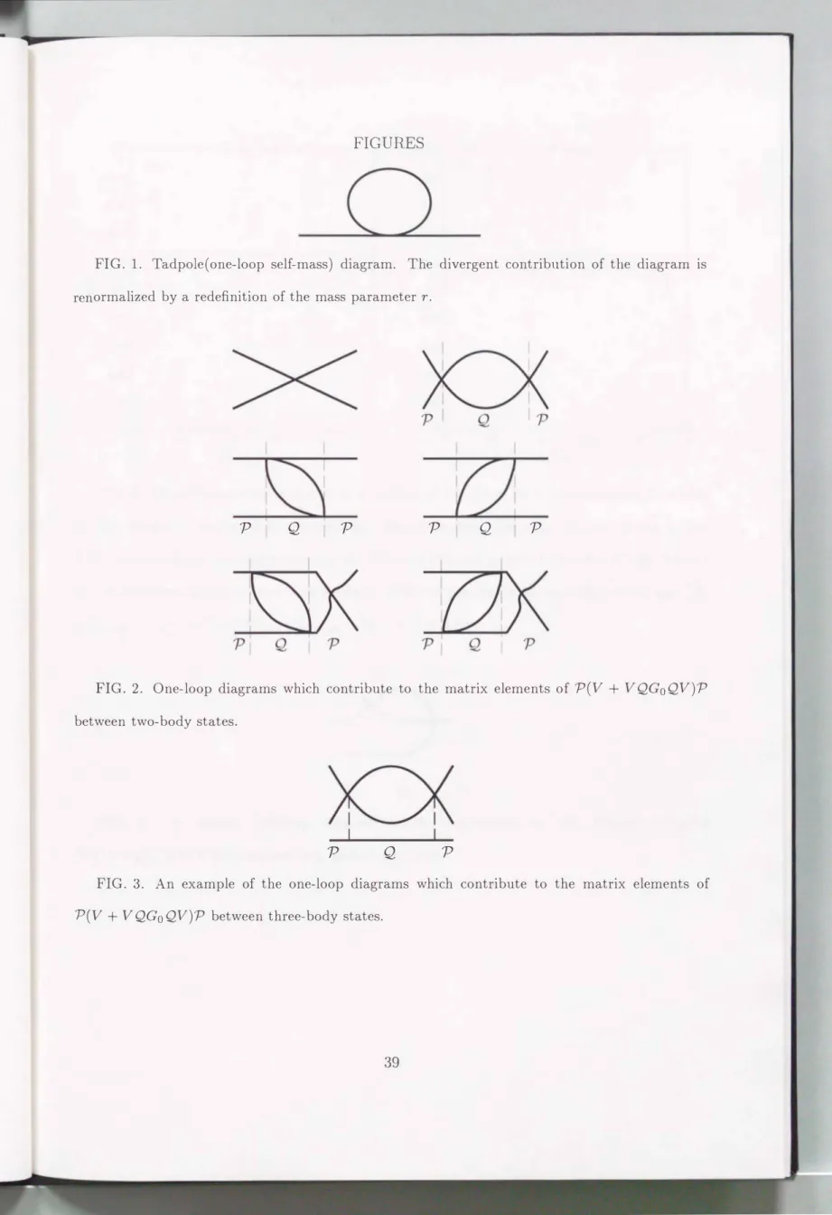
where the tadpole diagram

(

F ig.

1)

is removed by normal ordering the interaction term.

The Hamiltonian is rewritten as

H(Ao)

⁼

Ho

+ V,

00 00

V ⁼

L

^Vn,n +

L (

^Vn,n+2 + ^Vn+2,n

)

^,

n=2 n=l

(3.8)

(3.9)

(3.10)

where

A

J ^{4 dd-1k· n}

Vn,n

⁼

16(21f )d-In! [ g Jkt'] ^[ g ^{dd-!Pi ]}

x()

(

^{EA0 -}

�

E

( k; ₎

^-

�

^E

^{( p}

^;

⁾ )

⁽⁾

(

^EA0-

�

^E

^{( k}

^;

⁾ - �

^E

^{( P}

ⁱ

⁾ )

X

!k1, k2,P1,

^{· · ·}

,pn)(k3, k4,p1,

^{· · ·}

,Pn!,

A

J ^{4 dd-1k· n-1}

Vn,n+2

⁼

24(21f)d-l(n- 1)! [ g Jkt'] ^[ g ^{dd-!Pi ]}

x()

(

^{EA0 -}

E(kJ) - � _{E(p;) )}

()

(

^{EA0 -}

�

E

( k; ) - �

E

( p

^;

) )

X

!k1,p1,

^{· · ·}

,Pn-1)(k2, k3, k4,p1,

^{· · ·}

,Pn-11

where ^{EA0 =}

(Pi

⁺

A6)/2P+.

The total energy and momentum of an n-body state

!k1, k2, ... , kn)

satisfy the dispersion relation E =

(Pi

⁺

M2)/(2P+),

so the invariant mass

M

of the state is represented by the Jacobi variables,

xi

^and

si(i

^{= 1,}

... , n),

^as

where

n 2

⁺

M2

⁼

Lsi r >nr - 2

'

i=1 Xi (3.12)

(3.13)

One of the Jacobi variables is a dependent variable, since

2:.:�1 Xi

⁼

1

^and

L.:i=1 si

^{= 0}

in consequence of

P

⁼

2:.:�1 _ki.

The

xi

can vary from 0 to

1

and two components of the vector

si

⁼

(

^s

}

^{, s}

i)

from ^-oo to ^oo. The invariant mass M2 becomes minimum

n2r

^when

si

^{= 0 and}

Xi

⁼

1/n

^{for all}

i,

and it diverges at ^s

{

^{= oo or at}

^Xi

^{= 0.} The ultraviolet and infrared divergences are simultaneously excluded by the invariant mass regularization

M

^<

A0.

The Hamiltonian

(3.8)

has already been regularized with this, i.e., with the

step function () appearing in the momentum integrations. Here, it should be noted that the Hamiltonian does not include the zero-mode at all. The Fock vacuum is obviously an eigenstate of the Hamiltonian, indicating that the physical vacuum is trivial. A center of

mass motion is decoupled from internal motion in the Hamiltonian, ince it do s not contain any interaction between the two motions. This property is not broken by th invariant mass regularization.

The light-front quantization mentioned does not treat the zero-mode properly

[6,22].

As shown in Sec. III B, it is needless for the sy mmetric phase, but not for the brok n one. In principle, the zero-mode is treatable by quantizing the theory in a spatial box

-

L < x- � ^L under the periodic boundary condition, but in practice the procedure does not seem feasible, as mentioned in Sec. III C. The Ohio group suggests adding counter terms to the regularized Hamiltonian which does not contain the zero-mode

[12,19,23].

An aim of th present paper is to support the suggestion.

B. The second and third step of RG procedure

The second step of out RG procedure starts with dividing the finite transformation

(A

0 ---+

A)

into successive small transformation

(Ao

---+

A1

---+

···A).

For the nth small

transformation, G is obtained by solving G = G0 + G0 QV QG perturbatively, where the projectors

P

and Q are defined as

Plk1, k2, ... , kn)

=

B(EA0- c)lkl, k2, ... , kn) Qlkl, k2, ... , kn)

:=

B(E- EA0)1kl, k2, ... , kn)

(3.14) (3.15)

for any state having the total energy

E.

As shown in

(3.12), An

should be larger than

Jr,

so the one-body Fock state

(

with

M2

= r

)

can not be in the Q space. Any diagram including the one-body state then does not contribute to the Q-space Green function G.

In this paper we make one-loop approximation and neglect all irrelevant operators pro­

duced by the RG procedure as a reasonable approximation. A perturbative expansion of the Bloch-Horowitz Hamiltonian is then calculated up to second order in A, that is,

(3.16)

The second order correction

PV QG0 QVP

gen rates two-, four- and six-point vertices, but the six-point one is neglected, because it is an irrelevant op rator. Th correction i obtain d by calculating the matrix elements

(3.17)

separately.

Matrix elements of

P(V

+

V QG0 QV)P

between two-body Fock states are composed of four-point vertices displayed in Fig.

2.

In our all diagram, time flows toward the right. The longitudinal and transverse momenta are conserved at each vertex, and all particl s arc on shell. A net contribution of the diagrams becomes

(3.18)

The effective interaction has the same form as

V,

but with a new coupling constant

(3.19)

where

(

=

1/167r2

and A is a loop integral defined as

A=

J[�d:;i]83(P-�ki)F(k1,k2),

=

IA(An, r(An), Mi)- JA(An+l, r(An+l), Mi), _(3.20)

for

(3.21)

The loop integral A is obtained with an analytic function

IA

defined in Appendix A. The function depends on the cutoff,

Tn

and

Mi,

but not on

P.

Hereafter, it is assumed that

Ao

>>

Aphys

and

Mi

and

r n

are of order

Aphys·

For

An+l

>>

Aphys,

A= 47rln

An+l.

An (3.22)

Matrix elements of

P(V

+

VQG0QV)P

between three-body states are also calculated in a similar way. All diagrams contributing to the elements are also in Fig.

2,

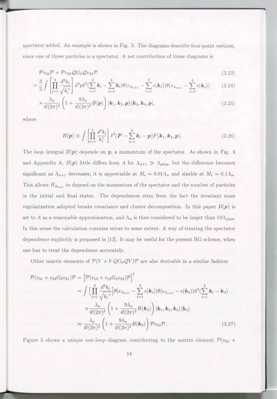
but with a

spectator added. An example is shown in Fig.

3.

The diagram d scrib four-point vertices, since one of three particles is a spectator. A net contribution of these diagrams is

where

(3.23) (3.24)

(3.25)

(3.26)

The loop integral B

(

p

)

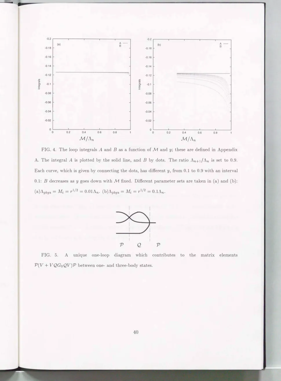
depends on p, a momentum of the spectator. As shown in Fig.

4

and Appendix A, B

(

p

)

little differs from A for

An+l

>>

Aphys,

but the difference becomes significant as

An+l

decreases; it is appreciable at Mi ⁼

0.01An

and sizable at Mi ⁼

0.1An.

This allows HAn+l to depend on the momentum of the spectator and the number of particles in the initial and final states. The dependences stem from the fact the invariant mass regularization adopted breaks covariance and cluster decomposition. In this paper B

(

^p

)

^is

set to A ^as a reasonable approximation, and

An

is then considered to be larger than

10Aphys·

In this sense the calculation contains errors to some extent. A way of treating the spe tator dependence explicitly is proposed in

[12].

It may be useful for the present RG scheme, when one has to treat the dependence accurately.

Other matrix elements of

P(V

+

V QG0 QV)P

are also derivable in a similar fashion:

(3.27)

Figure

5

shows a unique one-loop diagram contributing to the matrix element

P(

^v31 +

v33QGoQv3I)P.

No one-loop diagram contributes to the matrix lement

Pv13QG0Qv31P,

indicating that the element vanishes within the present approximation.

The effective Hamiltonian

HAn+I

thus obtained holds th same form as

HAn,

^{but with}

new parameters

Tn+l = Tn,

\ \ '21

An+l An+l =An+ 3(An

n

-- An

.

Taking the infinitesimal limit

8A

^----+

0, (An+l = An+ 8A)

leads to RG equations

(3.28) (3.29)

( 3

^.

3 0 )

For

A

^>>

Aphys,

the right hand side of the second equation tends to

3( A

^2• The right hand

side originally included a partial derivative

8IA (A, T(A)) I 8A

with

T(A)

fixed, but it has been replaced by

diAl dA.

The replacement is correct in this case, because of

dT IdA = 0.

^Even

if

dT IdA -=/= 0

just as in the case of subsection III C, one can make the same replacement

to derive RG equations at one-loop level, since

diAidA = 8IAI8A + O(n)

as a result of

dTidA = O(n).

The solution to

(3 . 3 0 )

is

T(A) =To,

A(A)- Ao

- 1- 3(AAol(47r)'

(3.31)

(3.32)

where

To= T(Ao), Ao = A(Ao)

and

A= IA(Ao, T(Ao))- IA(A, T(A)).

Expanding the solution

A(A)

in power of A, one can find that it contains not only contributions of the one-loop dia­

grams

(

Fig.

2)

but also those of the ladder diagrams, although for each small transformation only the one-loop diagrams have been taken into account.

The RG procedure ends up with the scale transformation

T

of

(2.9)

and

(2.10),

where it is assumed that there exists only a Gaussian fixed point in the present model. The transformed Hamiltonian

H�0

⁼

T[HA]

has parameters

A

'(A)

⁼

A(A), r'(A)

⁼

( ;,. )

²

^{r(A), (3.33)}

The running coupling X

(A)

depends not only on

A,

but al o on th eig nvalu

Mi

of

HAo

through A. In the limit

A----*

oo, however, the coupling tends to

-\(A)=

^Ao

1-

3(-\0ln(A/A0)/(4n)' (3.34)

indicating no

Mi

dependence. The mass parameter

r(A)

present in

HA

has no

A

dependence and then equal to the lowest mass

M1,

so that the corresponding param ter

r'(A)

in the transformed Hamiltonian

T[HA]

behaves as

M1A0/ A.

We then draw a flow diagram for the lowest state by setting

Mi

⁼

M1

⁼

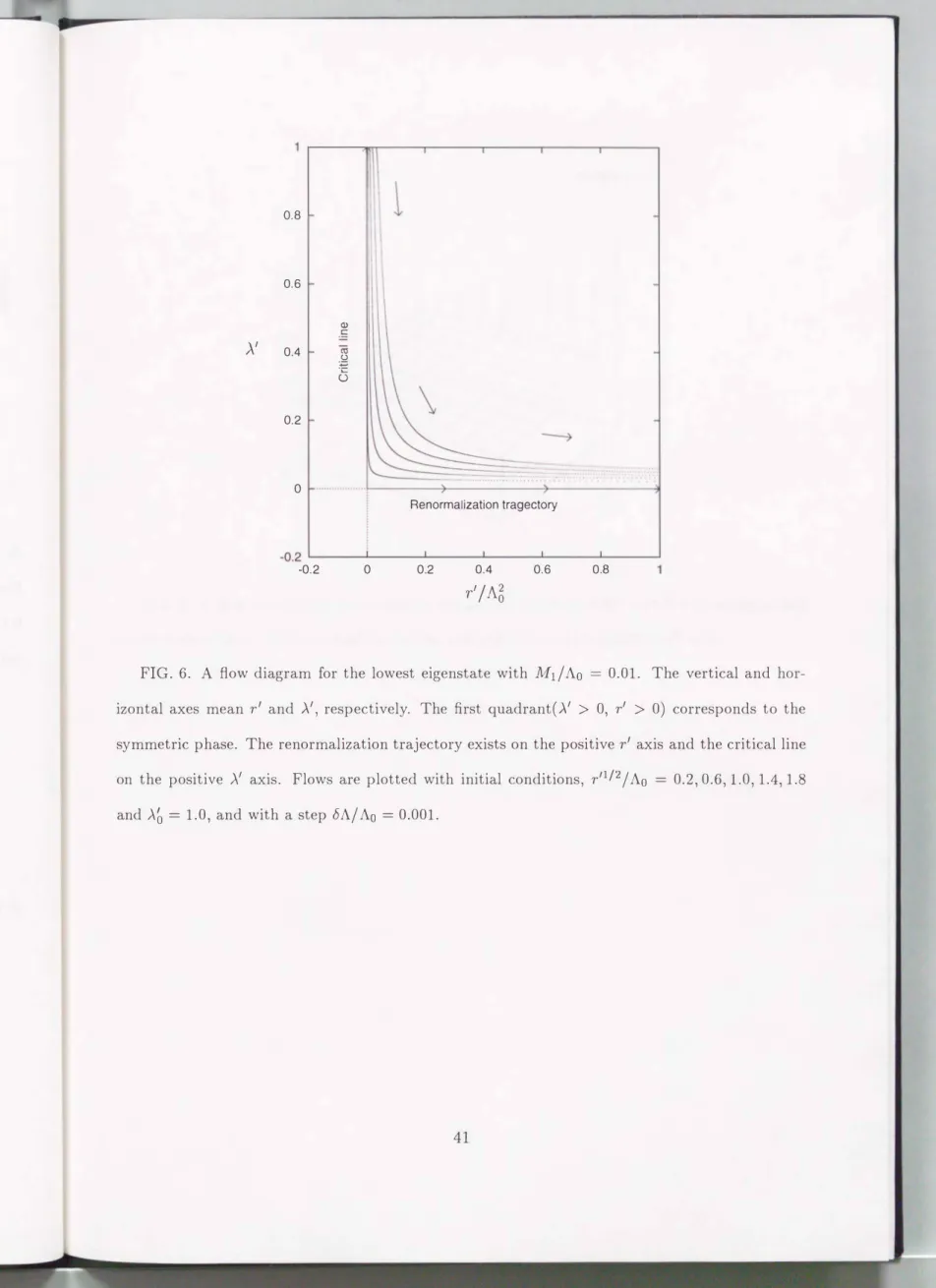
Mphys

in A as a renormalization condition. The diagram presented in Fig. 6 shows, as expected, that there exists a renormalization trajectory on th positive r ' axis. On the axis X is always zero, indicating that the present model is trivial.

Once the trajectory is found for the lowest state, renormalization trajectories for other states are obtainable from the one for the lowest state by replacing

M1

by invariant masses of the excited states, if they are known. In the present case, such a state depend nee does not appear as a reflection of the triviality, that is, all the trajectories exist on the positive r'

aXlS.

There appear two phases in Fig. 6; a critical line between the two is on the positive X _axis. A phase present in the first quadrant

(-\'

2:: 0 and r' 2:: 0

)

is symmetric for the

reflection

¢

^----*

-¢,

since the effective Hamiltonian holds the symmetry. Another phase appearing in the second quadrant is then considered to be a broken one. The present cutoff Hamiltonian

HA0,

however, is not applicable for the phase, since Fock states with negative

r are not physical in the sense that tachyons come out. In general, light-front Hamiltonians are different between the phases, while their vacua are always equal to the Fock vacuum.

This is explicitly shown in two-dimensional

¢4

^model

[7-9];

for the symmetric phase the Hamiltonian contains oscillatory modes only, while for the broken phase it includes both zero and oscillatory ones. The Hamiltonian for the broken phase has a new mass term produced by the zero-mode in addition to the original one r, so one can define Fock states

with the sum, even if

r

is negative. Further discu sion on th brok n phase is mad in Sec.

III C.

C. The RG equations for the broken phase

The RG equation

(3.30)

is valid for the symmetric phase, but not for the broken one, because the canonical Hamiltonian is tachyonic in the broken phase, as shown in S c. III B.

The failure stems from the fact that the present HAo does not contain the zero

(k+

⁼

0)

mode. It is known that there are two kinds of zero-mode, a constant and a onstrained zero-mode. The zero-mode is responsible for the spontaneous symmetry breaking, because the order parameter cannot become nonzero without the zero mode. Hence the present HAo is valid only for the symmetric phase which has a vanishing order parameter.

There are two ways of finding a Hamiltonian valid for the broken phase. One way is to treat the zero-mode explicitly

[6-9).

For this purpose

¢4

theory is usually quantized in a

spatial box

-

L <

x-

< L under the periodic boundary condition, so that the z ro-mode is separated from the oscillator ones. The resulting bare Hamiltonian is different from the present Hamiltonian in the sense that the bare Hamiltonian contains not only the oscillator modes but also the zero-mode. The zero-mode is an operator-valued function of the oscillator modes, since the zero-mode satisfies a constraint

[6)

j_

_-L L

dx- { (r-ai)¢(x)+ �¢3(x) _3. } ^{=0. (3.35)}

This has been obtained by integrating the equation of motion over

x-.

In general, it is not easy to solve the operator valued nonlinear equation for the zero-mode without perturbation in order to treat spontaneous symmetry breaking. A trial is reported for

¢4

model in two dimensions. In

[7-9),

the equation is symmetrically ordered and approximately solved under the Tamm-Dancoff truncation. However, it is not clear how we should order the equation, since the zero-mode is not a dynamical operator.

Another way is to add counterterms to the canonical Hamiltonian which has no zero- mode

[12,19,23].

Only the zero-mode can make the order parameter

(Oj¢j0)

nonzero. This

means that the system has to sit in the bottom of the effective potential, a oon as the zero-mode is discarded from

¢.

So we introduce a constant zero-mode

v,

^{and hift}

¢(x)

^as

¢( x) = <p( x) + v,

and determine a value of

v

as a function of original running parameters

r

and

A.

In terms of the shifted field

<p

the Lagrangian density b comes

where

u

= vr + 1v3, A

3.

m=r+- AV2

2 ' ^{g =VA,}

(3.36)

(3.37)

and a constant term has been discarded, because it is irrelevant to physics. The light-front Hamiltonian is then

(3.38)

where normal ordering is assumed. A linear term in

<p

does not appear, since the constrained zero-mode is removed by a small longitudinal cutoff, i.e., invariant mass regularization.

Following the RG procedure shown in the previous subsections, one has RG equations for

m, g,

^and

A.

^RG equations for new parameters are

By taking infinitesimal limit An+l ⁼ An

+

^{8A, 8A ---+}

0,

^{we have}

dm 2

AdA=

(g'

d

g

AdA

= 3(Ag,

Ad

A = (A2

dA

3 '

where

A

is replaced with

41f

^ln

(

^A

/

^A0

)

. The solutions to

(3.42)

are obtained as

(3.39) (3.40) (3.41)

(3.42)

m(A) - m - �A v2 � Aov5

- 0 3

°

0

+

3 1

+

3( Ao ln(A0/ A)'

(A)- go

g - 1

+

3(A0 ln(A0/ A)' A(A)

⁼

Ao

1

+

3(A0 ln(A0/ A)"

Cutoff dependence of the original parameters is

v(A)

⁼

vo,

r(A) - r �A v2 - � Aov5

- 0

+

6

°

0 6 1

₊

3( Ao ln(A0/ A)'

A(A)- Ao

- 1

+

3(A0 ln(A0/ A)'

(3.43) (3.44) (3.45)

(3.46) (3.47) (3.48)

where all parameters at

A

⁼

A0

are characterized by a subscript

"0".

Th corresponding parameters,

v', r',

and

A',

present in

T[HA]

are then obtained by

v'(A)

⁼

( �) v(A), r'(A)

⁼

( �) 2 r(A), A'(A)

⁼

A(A). (3.49)

The parameter space of the broken phase is larger than that of symmetric phas . The degrees of freedom of independent parameters should be same in both phases. It is natural to suppose that there exist a relation, which is independent of renormalization, among the parameters in the broken phase. By using these solutions

(3.46)-(3.48),

we observe that the sum

6r

+

Av2

does not depend on the cutoff

A

(3.50)

indicating that a quantity c =

6r

+

Av2

is RG invariant. Thus,

v

is obtained as a dependent variable. This is a natural result of the fact that the original theory includes only

r

and

A

as physical parameters. The relation between

v

and the physical parameters should be unique.

In fact, c is determined as follows. The relation becomes

6r'

+

A'v'2

⁼

cA2

for parameters

v', r',

and

A1

which include rescaling effect, and it forms a group of surfaces, each with different c, in the parameter space. Only a surface with c ⁼

0

contains th critical line

(

the positive

A

axis

)

between the broken and symmetric phases. The line is a border of the surface, since

r' = ->..'v'2 /6

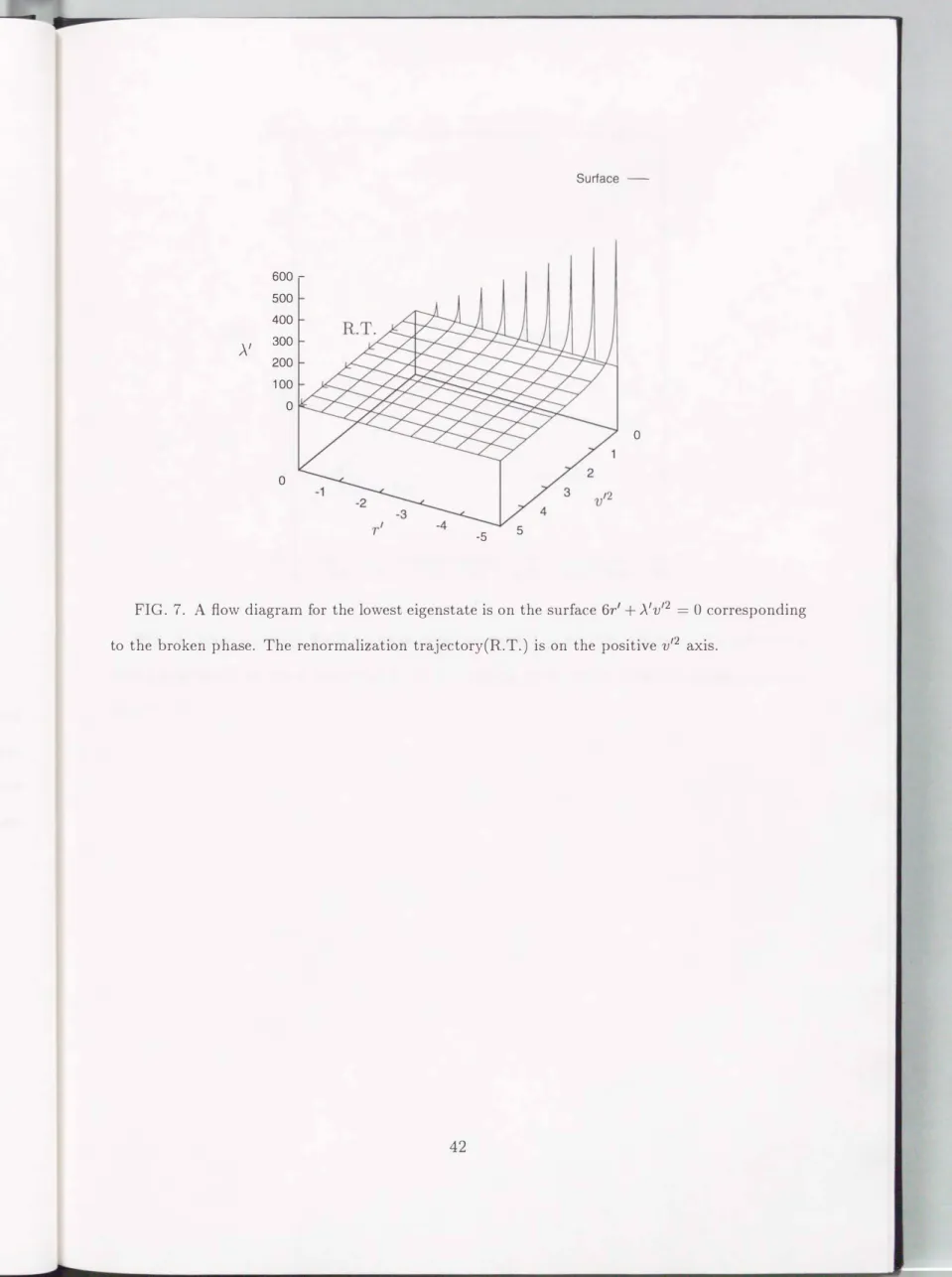
< 0 for positive A'. The surface can be regarded as the broken phase, since it can be connected to the symmetric one on the critical line. The surfac is depict d in Fig. 7. The asymmetric Hamiltonian for the broken phase is defined on the RG invariant surface 6r +

>..v2 =

0. The effective potential should become minimum on the surface, and it is really confirmed in Sec. III D. The renormalization trajectory is on the surfac , as expected. Perry and Wilson also found the same relation without calculating the effective potential. Their derivation is essentially equivalent to ours, although c is set to z ro a priori in their derivations.

D. Covariant perturbation theory and effective potential

The RG equations (3.42) based on the present light-front Hamiltonian formalism are compared with those on the covariant (equal-time) perturbation theory. For this purpose, we use a cutoff on the Euclidean momentum,

k2

<

A 2,

and make the same approximation, that is, the one-loop approximation and dropping irrelevant operators. The resultant RG equations are

A-du =

^__

(g_A _ 2 dA

1 +

TJ'

A dm = (g2 - _(>.. _ A_2 dA

( 1 +

TJ) 2

1 +

TJ ' A dg = 3(>..g

dA

(1 +

TJ)2' A-d>..= 3(_A2

dA

(1 +

TJ)2'

^(3.51)

where

TJ

=

m/ A 2.

Inserting relation (3.37) into (3.51) yields RG equations for the original parameters,

AdA= dv

0,

A-dr = ((>..v)2

^__

(>.._A _ 2 dA

2 ( 1 +

TJ) 2

1 +

TJ' A-d.A = 3(.A2

dA

(1 +

TJ)2•

^(3.52)

In the derivation of

(3.52)

^from

(3.51),

the number of quations i reduced from

4

^to

3.

One of four equation in

(3.51)

is thus not indep ndent under th condition

(3.37).

^For

A

much larger than m and Mi,

(3.52)

agre with

(3.42),

^except

(3.52)

n wly have a t rm

-(.XA2/(1 + ^TJ)

in its second equation. The term comes from the tadpole (Fig.

1),

but in the present formulation the self-mass has already been included in th rna s parameter

T

by taking the normal ordered Hamiltonian. Hence, the RG equations obtained in th light­

front Hamiltonian formalism are essentially equal to Eqs.

(3.52)

cal ulated in the covariant perturbation theory. Of course, the two RG equations are not identical except the large

A

limit, because regularization schemes are different between the two formulations. The light-front perturbation theory is formally equivalent to th covariant on

[24],

if the same regularization scheme is taken. In fact, as soon as the k- integration is made in the covariant formalism, one finds a direct connection between diagrams obtained in the covariant th ory and time-ordered ones in the present formalism.

The equality guarantees that within the framework of the light-front Hamiltonian formal- ism we can calculate the effective potential through the following ordinary procedure. In the covariant perturbation theory, the effective potential

V[¢cJ]

is obtained as

TR¢�1/2 + .\R¢�1/4!

within the present approximations, where

TR

^and

AR

stand for renormalized quantities and

<Pc1

for the classical field, that is, the vacuum expectation value of ¢. The renormalized quantities are solutions

T(A)

and

.\(A)

at the small

A

limit to RG equations

(3.52)

under the condition v = 0, because

TR(.XR)

are just the sum of one-particle irreducible diagrams

produced by an interaction

.\¢4

with

2( 4)

external lines. In fact, the solutions are

3 2 { ^{A5 + To A5} } ²

.X(A)IA=o

⁼

Ao- -(.\0

ln

- A2 + O(n )

^,

2 To 0 +To

1 { ^{2 A2 +To} } ²

T(A) IA=O =To - -( Ao A0 -To

^ln

+ O(n )

,

2 To

(3.53) (3.54)

at the one-loop level, and they agree with

TR

^and

AR

directly calculated with the covariant perturbation theory. Also in the light-front Hamiltonian formalism,

TR

^and

AR

are obtained from the solutions

(3.46)(3.47)(3.48)

by setting

A

to the small

A

limit and v to zero. The

AR

thus obtained contains not only contributions of the one-loop diagrams (Fig.

2)

^{but also}

where

a= 3(

^ln

A (A

^rv

0). (

ⁱ

)

Conversely,

(3.56)

The condition

dV[<Pc�]/ d<Pc1

⁼

0

on which the effective potential is minimum leads to

(

ⁱⁱ

) 6rR

⁼

-.AR<P�1•

^RG equations

(3.52)

are now solved under the initial conditions

(

ⁱ

)

^and

(

ⁱⁱ

)

^;

of course

<Pc1

is identified with

v.

As mentioned in Sec. III C, ^{c =}

6r(A) + .A(A)v2(A)

is RG invariant. For any

A

it becomes

av2,A2

C = _{_}

0 R

1 + aAR' (3.57)

because of relations

(

ⁱ

)

^and

(

ⁱⁱ

)

. In the large

A0

limit, the quantity

a

diverges, so that ^c tends to

-v5 AR

^for

AR

⁼

.A0/ (1

^-

a.A0)

^----7

0.

^{Hence, c} is zero in the limit, as far as

v0

^is

finite. This is a reflection of the fact that

AR

is forced to vanish in the limit, that is, the present model is trivial. The condition for the system to be in the bottom of the effective potential is then ^{c =}

0.

It agrees with the result shown in Sec. III C.

IV. NONPERTURBATIVE RG SCHEME

The first principle of RG is to find a flow which g1ves the same physics. It is not easy to calculate the effective interaction part of the Bloch-Horowitz Hamiltonian directly for our practical purpose of nonperturbative renormalization and we have to avoid energy dependences of renormalization, then we consider another approach. In our framework, we can draw RG flows by calculating spectra. We regularize the LF Hamiltonian with the basis function regularization and try to calculate the critical surface.

A. Three-dimensional real scalar model

First, We derive perturbative RG equation for mass parameter in the thr -dim nsional real scalar model. We assume that the canonical Hamiltonian is given by

Hs =

J

d ² x

( -(81_¢ ^{2 1 )}

^{2 +}

²

^{r 2}

-¢

⁺

-¢ ^4!

^{A 4 + -w}

^6! ¢ 6)

^.

^{( 4.1)}

The normal ordering is taken here. This is equivalent to renormalization of tadpole diagrams by redefining parameters. We have to include various kinds of marginal and irrelevant inter- actions to renormalize all new interactions produced by RG transformations. Our Hamilto- nian is assumed to have three interactions in Eq.

( 4.1).

Let us consider mass r normalization perturbatively in order to guess where the critical line exists. The mass renormalization is most important, because ^r is most relevant to mass spectra. It is the free part which mainly contributes to mass spectra especially in the perturbative region. The RG equation for mass r is given in perturbation theory as

( 4.2)

where

(4.3)

It is understood implicitly that the loop integral is made in the Q space. The factor L is produced by rescaling the new cutoff An+l to the original cutoff An. By changing variables to Jacobi coordinates,

0 < Xi <

1,

- OO < Si < 00,

where all intermediate states have a common total momentum K, the integral B becomes

( 4.4)

where

M

is an external mass

(

an eigenvalue of Hamiltonian

)

and

Mint

a mass in the inter- mediate Fock state,

(4.5)

It is assumed that the external mass

M

is small compared to the cutoff scale. The int rmedi- ate mass

Mint

is large because it sits in the higher mass spac Q. Then,

M2

is much smaller than

Mi;t.

This assumption is reasonable for the purpose to calculate critical lin and draw a phase diagram. We can observe from C being negative that limn-+oo

r

n ⁼ oo if the initial value

ro

is sufficiently large and limn-+oo

r

n ^{= -}oo if the initial value

r0

is small. That is, there exist a critical line

r

⁼

rc(.A)

in the first quadrant of the two dimensional parameter space

(r, ..\),

and r >

rc(.A)

and

r

<

rc(.A)

correspond to symmetric and asymm tric phases respectively. In the asymmetric phase, the canonical Hamiltonian

( 4.1)

is tachyonic, i.e., square of eigenmass is not bounded from below although Hamiltonian should be positive definite. Positivity of the spectrum is restored by expanding the field

¢

around th correct VEV v. Substituting

¢(x)

⁼

<p(x) +v

into Eq.

(4.1),

we have

where the new mass parameter is

and the new coupling constants are

93 =

(.A + -)v,

wv2

6

94

=.A+--,

wv2

2

^{95 = wv, 96 = w.}

( 4.6) (4.7) ( 4.8)

(4.9)

(4.10)

The v is just a free parameter at this stage. We have three parameters in the symmetric Hamiltonian Hs and four in the asymmetric one HA. The RG parameter space for HA is larger than that for Hs. The v should be a function of the original three parameters belonging

to Hs, that is, there should exist an RG invariant relation among the four parameters.

Actually, following our previous work

[17]

for the real scalar model in four dimensions, we can find out the same RG invariant relation 6r +

.Xv2

⁼ 0 also for the thre -dimcn ional case, with perturbative renormalization at one-loop order, if the

¢6

interaction is n gl ted.

The neglect of the marginal operator will be justified by numerical analyses hown later.

The RG invariant relation forms a surface in the parameter space for HA· All asymmetric Hamiltonians on the surface describe physics for the brok n phase. All running param ters on the surface go to zero in the limit A ----* 0 which corresponds to infinite iterations of RG transformation, satisfying the RG invariant relation 6r +

.Xv2

⁼ 0. The Hamiltonian HA thus gives massless spectrum in the limit. All Hamiltonians on the surface converg to the same massless Hamiltonian in the limit, indicating that HA gives massless sp ctrum at any point on the surface. We will continue our analysis assuming that the broken phase would be found nonperturbatively by searching massless eigenvalues.

B. Basis function regularization

In general, we can express an arbitrary state in the Fock space such as

( 4.11)

where

P

is the total momentum of the state and the wavefunction 1/Jn is symmetric under exchanges of arbitrary two momenta. The limit

NTD

^{----* oo} corresponds to the full theory and the state is normalized as

(w(P)Iw(Q))

⁼

82(P- Q). ( 4.12)

We will set a certain small number to

NTD,

which is called the Tamm-Dancoff approximation.

In this paper, the Fock space is truncated up to three body states

(NTD

⁼

3).

According to the variational principle, the mass spectrum in the truncated Fock space is given by solving

(

diagonalizing

)

the Einstein-Schrodinger

(

ES

)

equation

(4.13)

We introduce a cutoff

A

and show the pre ent regularization sch me later. All quantities belonging to the model are measured in units of the

A

and attached tild . In unit of the cutoff, eigenmass and running parameters are

then

!Jn

⁼

9n/ A ^(6-n)/2.

(4.14)

( 4.15)

The ¢6 interaction is marginal as shown in Eq.

( 4.15).

We will check the marginal coupling dependence of the critical line in the next section. The momentum is also redefined as

(4.16)

where 0 < xi <

1

since

kt

^> 0. In this rescaled notation, the normalization condition Eq.

(4.12)

of the wavefunction becomes

( 4.17)

where

(4.18)

and the rescaled wavefunctions are

n-1

,(/;n(xl,x2,···,xn)

⁼

(P+A)-2 'I/Jn(kl,k2,···,kn)· (4.19)

The ES equation in the rescaled notation is given in appendix B. It can be seen that the ES equation does not depend on the longitudinal momentum

p+

and the cutoff

A.

Regularization of transverse momenta and discretization of Fock space are closely related to each other. The regularization of the Hamiltonian is realized as a boundary condition of the wavefunctions. That is, we solve this eigenvalue problem, keeping the constraint that

the transverse component of

{/;3

is zero at edg s

(Xi

⁼

^{-1, 1).}

Th ES equation i regularized with the naive transverse cutoff,

-A _<

kij_

< A

� -1

<

Xi

<

1, ( 4.20)

since the ultraviolet divergence is caused by the transverse loop integral. The Fock space is discretized by expanding the wavefunction in terms of basis fun tions in th morn ntum space

( -1

<

Xi

<

1, 0

<

Xi

<

1),

where

n n

L: x i = 1, I: xi= Pj_,

i=l i=l

(4.21)

( 4.22)

and S1,2,

... ,n

is a symmetrizer. The NL

(

n

)

and NT

(

n

)

are taken sufficiently large so that the eigenvalue of the ground state can converge. Longitudinal basis functions are

fk(x)

=

x{3(n)+k, 0

<

x

<

1,

for

0

<

{3(

n

)

<

1

and transverse basis functions are

( 4.23)

( 4.24)

The variational parameter /3( n

)

is tuned so that the ground state takes minimum igenvalue.

The behavior of the three-body wavefunction near the edges

(

x

= 0, 1)

is important because of the kinetic term proper to LF

[25,26].

The coefficients

aL�)

are determined by diagonalizing the Hamiltonian in the momentum space spanned by the basis functions. Mathematically, Eq.

( 4.13)

has exact eigenvalues only in the case the functional space is expanded in terms of the complete set of basis functions. We can get only upper bounds of eigenvalues, since the wavefunction is expanded in terms of incomplete basis functions in this calculation.

However, we expect that the spectrum is described accurately for low-lying states, since shapes of the wavefunctions are simple; for example, the calculated wavefunction of the ground state has no node.

In this paper, a phase diagram which includes rescaling effect is evaluated, in accor­

dance with Wilson's RG prescription [13]. It is not need d to vary the cutoff because th transformed cutoff is rescaled to the original one in this RG. Param ter s ts whi h give the same eigenvalue are calculated for a fixed cutoff.

The wavefunction renormalization is neglected in this calculation, i.e., Zcp ⁼ 1. Th phase diagram is dominated by the Gaussian fixed point, since the field is reseal d according to the canonical dimension. In order to find a non-trivial fixed point, w have to consider th wavefunction renormalization. These two phase diagrams, which have trivial and non-trivial fixed points, describe different theories. Our result makes sense as the theory dominat d by the Gaussian fixed point.

In this calculation, the total transverse momentum of the eigenstate is set to zero,

F1_

= 0, and

N1,T(n)

= 3 in Eq. (4.21), which is sufficiently large so as to give a convergent spectrum.

C. Numerical results

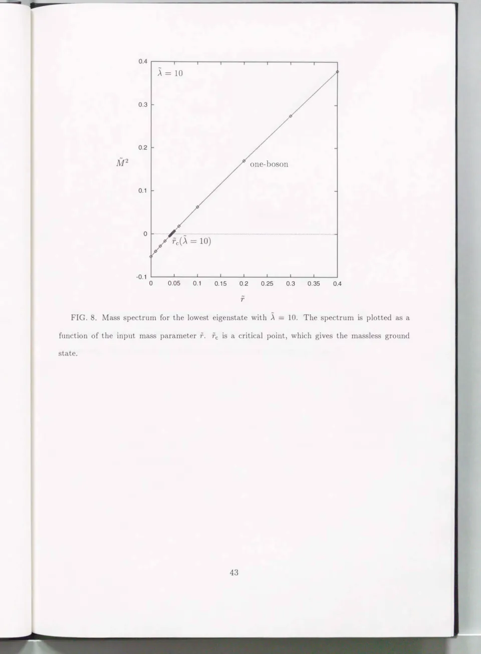
Mass spectrum is plotted in Fig. 8 for the case A ⁼ 10 and w ⁼ 0 without introducing v.

No multi-bosonic bound state is found in this calculation. We can observe a massless point

rc(�

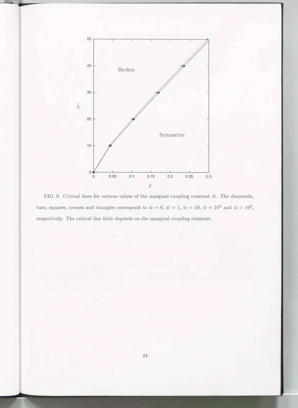
= 10). The point is called the critical point. We can draw the critical line by connecting

the critical points which are calculated for various A. The critical line is plotted in Fig. 9 for five values of marginal coupling constants, w ⁼ 0, 1, 10, 102, 103. Values of two parameters

r

and

�

which form the critical lines are tabulated in table I for each w. The depend nee of the line on w is weak. This is consistent with our intuition based on perturbative analysis, i.e., the dependence of the line on higher power operators in cp may be week. After this, we will switch off the marginal coupling w ⁼ 0, and draw the phase diagram of three running parameters, v,

r

_{and A near the v} = 0 plane.

The lowest eigenmass is zero on the line, corresponding to an infinite correlation 1 ngth in the statistical theoretical language. The spectrum of the canonical Hamiltonian is not bounded from below in the left region of the critical line. We then conclude that excited

states are lighter than the ground state in the region if we solve th anonical Hamiltonian as it is. This is a result of the mass renormalization eff ct xplain d in th section IV A.

The true Hamiltonian should be positive definite even in the l ft region of th ritical line.

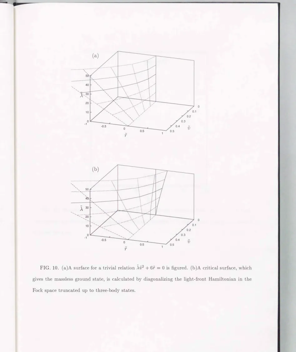
It is natural to introduce the VEV in the broken phase in order to con truct a po itiv definite Hamiltonian. The symmetry has to be spontaneously brok n for the p ctrum to keep positive. Figure 10

(

^a

)

shows a relation

�v2

^{+ 6r =} 0 among thr paramet rs

v,

^r

and A, which is given by perturbative RG calculations at one-loop ord r· the detail of th calculations is shown in

[

¹⁷

]

for the case of the four-dimensional scalar model. W an s the critical line on the positive A axis, which is trivial because no renormalization ffect is included. In Fig. 10

(

^b

)

, a critical surface is drawn. The surface is calculat d by searching points which give massless spectrum in the three-dimensional parameter space

(v,

^r,

�).

Positivity of the Hamiltonian is restored by introducing

v.

Compared to the surface

(

^a

)

ⁱⁿ

Fig. 10, the surface

(

^b

)

slants to the positive r direction if

v

is small and to the negativ direction if

v

is large, as a result of renormalization effects.

Components of the ground state wavefunction on the critical line shown in Fig. 9 are plotted in Fig. 11 in order to confirm whether the TD approximation works well or not. One­

and three-body wavefunction probabilities are plotted as a function of A on the critical line.

The three-body component is very small even for comparatively strong coupling

�.

^This

means that the spectrum does not change near the critical line even if higher Fock space contributions are included in the calculation. This is true also in region far from th critical line, when the VEV is zero. The three-body component of the ground state wavefunction tends to decrease, as mass parameter increases with coupling constant fixed, because taking large mass parameter is effectively the same as taking weak coupling constant.

Next, we investigate TD dependence of the critical surface. Figure 12 shows wavefunction components of the ground state on the intersection between the critical surface and the A ⁼ 50 plane. The coupling constant is set to the largest value in this calculation. One- and two-body components are dominant and three-body component is small also in this case.

The two-body component increases rapidly near

v

⁼ 0.1, whereas the three-body component

increases slowly and keeps the value around a few percent. It is exp cted near th

v ⁼

0 plane that the Tamm-Dancoff approximation is good.

V. SUMMARY AND DISCUSSIONS

Our results of perturbative RG in the four dimensional real scalar mod l ar ummarized as follows.

(i) The present RG scheme based on the Bloch-Horowitz effective Hamiltonian is quite practical, because the scheme is free from the "vanishing energy d nominator" problem and the

Ei

dependence of the effective Hamiltonian causes no big problem in practic . Whil RG equations are easily derived in perturbation theory, RG flows d pend on eig n nergics

Ei

of

HAo,

since so does the effective Hamiltonian. The state dependence is negligibl for

A

much larger than

Mi.

(ii) Renormalization group (RG) equations for mass

r

and coupling

A

ar derived at on - loop order, where all irrelevant operators generated by RG transformation are remov d as a reasonable approximation. The invariant mass regularization [12,21] is adopted in this paper, but it breaks covariance and cluster property, so the running mass and coupling constant depend on momenta of spectators if they exist. The dependence is, however, very weak, as long as

_A

is at least several times larger than -/T ^and

Mi

which are assumed to be of order the physical mass scale

Aphys·

So it is neglected as a reasonable approximation in this paper. The regularization also excludes the zero-mode (a mode with zero longitudinal momentum) from the canonical Hamiltonian. The zero-mode is responsible for spontaneous symmetry breaking, that is, the order parameter (OI¢10) for the

Z2

symmetry never becomes nonzero without the mode. This means that the RG equations calculated with the initial cutoff Hamiltonian are correct only for the symmetric phase. In fact, a flow diagram drawn with the RG equations shows not only that two phases exist, but also that tachyons come out in the broken phase.

(iii) In light-front field theory, Hamiltonians are different between the two phases, while