Branch-and-Bound Algorithms for Variable Selection and Shortest Vector Problem
木村, 圭児
http://hdl.handle.net/2324/2236041
出版情報:九州大学, 2018, 博士(機能数理学), 課程博士 バージョン:
権利関係:
Doctoral Thesis
Branch-and-Bound Algorithms for Variable Selection and Shortest Vector Problem
Keiji Kimura
A thesis submitted in fulfillment of the requirements for the degree of Fuctional Mathematics
in the
Graduate School of Mathematics
February 15, 2019
(MINLP) problems have increased significantly in the past 20 years. State-of-the-art optimiza- tion software, especially, is available for many optimization problems, and it is widely used by researchers and practitioners. However, the computational costs of MINLP problems are much higher than that of mixed integer linear problems even though such software is used. In addition, it does not make use of every property of a given optimization problem because it is regarded as general-purpose optimization software. On the other hand, an MINLP solver purpose-build for a specific problem occasionally achieves good computational performance.
Herein, we propose effective branch-and-bound algorithms to solve two problems: variable se- lection and shortest vector problems. A branch-and-bound algorithm is a design paradigm for discrete and combinatorial optimization problems, and it consists of some components, such as relaxation, branching, and heuristic methods. We take advantage of the structure and prop- erties of the problems to improve these components in terms of computational performance.
We show numerical experiments pertaining to the proposed algorithms and examine how they outperform state-of-the-art optimization software.
Variable selection: Finding the best statistical model for a given dataset is one of the most important problems in statistical applications (e.g., linear and logistic regression). This prob- lem is called variable selection, and solving it leads to various benefits. We focus on direct objective optimization which computes the best subsets of variables in terms of a given ob- jective function. Computation of all candidates is impractical because the number of them is exponentially large. We formulate this optimization as an MINLP problem, which corresponds toℓ0-penalized variable selection. To solve it efficiently, we develop some components related to a branch-and-bound algorithm, for example, relaxation, a heuristic method, and branching rules. Moreover, we explain the application of the MINLP problem.
Shortest vector problem: The security of lattice-based cryptosystems is based on the hard- ness of problems on lattices. One of the most studied problems on lattices is the shortest vector problem (SVP), which searches for the shortest non-zero vector in a given lattice. This prob- lem is known to be NP-hard, and it has been generally researched in the field of cryptology.
Herein, we apply mathematical optimization to SVP. From the point of view of optimization software, SVP contains an intractable constraint, and it cannot directly be solved via optimiza- tion software. To handle the constraint, we develop ingenious branching and relaxation. In addition, we propose a heuristic method to find feasible solutions of subproblems. We examine computational performance of the proposed branch-and-bound algorithm. To this end, we propose two convex integer quadratic programming approaches using state-of-state-of-the-art optimization software.
Keywords: Mixed integer nonlinear programming, branch-and-bound algorithm, variable se- lection, shortest vector problem.
1 Introduction 3
1.1 Mixed integer nonlinear programming . . . 3
1.2 Variable selection . . . 4
1.3 Shortest vector problem . . . 5
1.4 Contribution . . . 6
2 Branch-and-Bound Algorithm 8 2.1 MINLP problems . . . 8
2.2 Algorithm design . . . 9
2.3 Basic components . . . 10
3 Direct Objective Optimization in Variable Selection 12 3.1 Overview . . . 12
3.2 Customized branch-and-bound algorithm . . . 13
3.2.1 Relaxation . . . 13
3.2.2 Heuristic method based on stepwise methods . . . 15
3.2.3 Most frequent branching and strong branching . . . 16
3.3 Applications . . . 18
3.3.1 Application 1: AIC minimization for linear regression . . . 18
3.3.2 Application 2: AIC minimization for logistic regression . . . 20
3.3.3 Effective handling of data structure . . . 21
3.4 Numerical experiments . . . 25
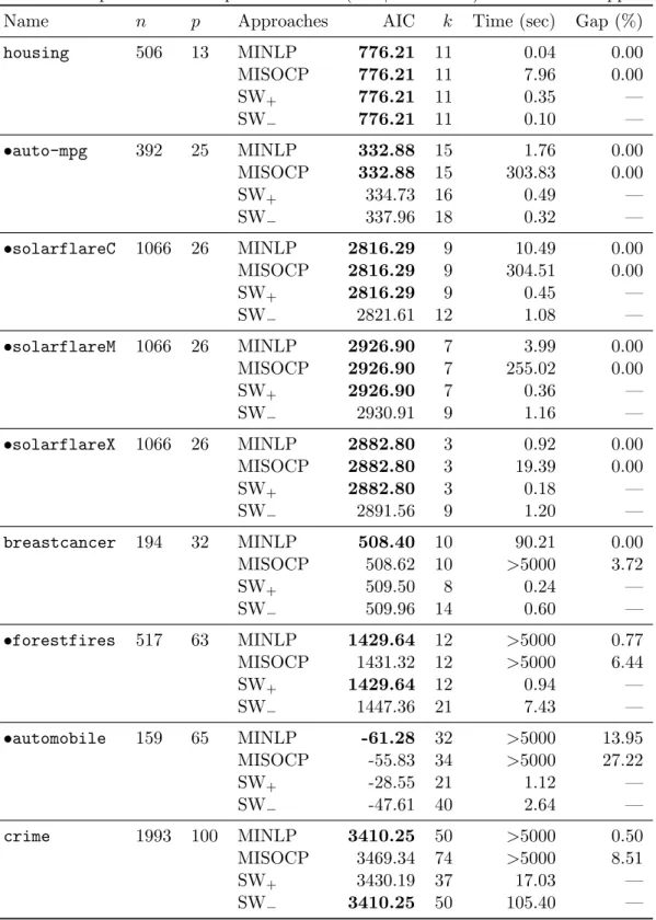
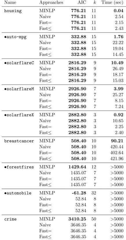
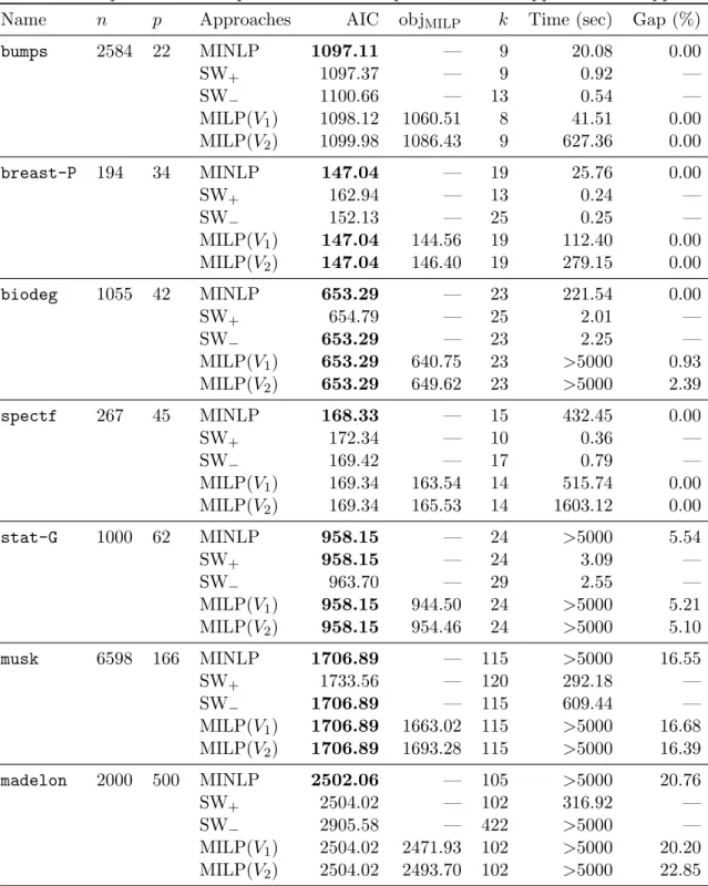
3.4.1 Application 1: Comparison with stepwise methods and MISOCP approach 26 3.4.2 Application 1: Comparison with MIQP approaches . . . 27
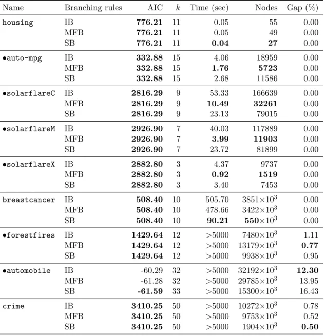
3.4.3 Application 1: Comparison of branching rules . . . 29
3.4.4 Application 2: Comparison with stepwise methods and piecewise linear approximation approach . . . 30
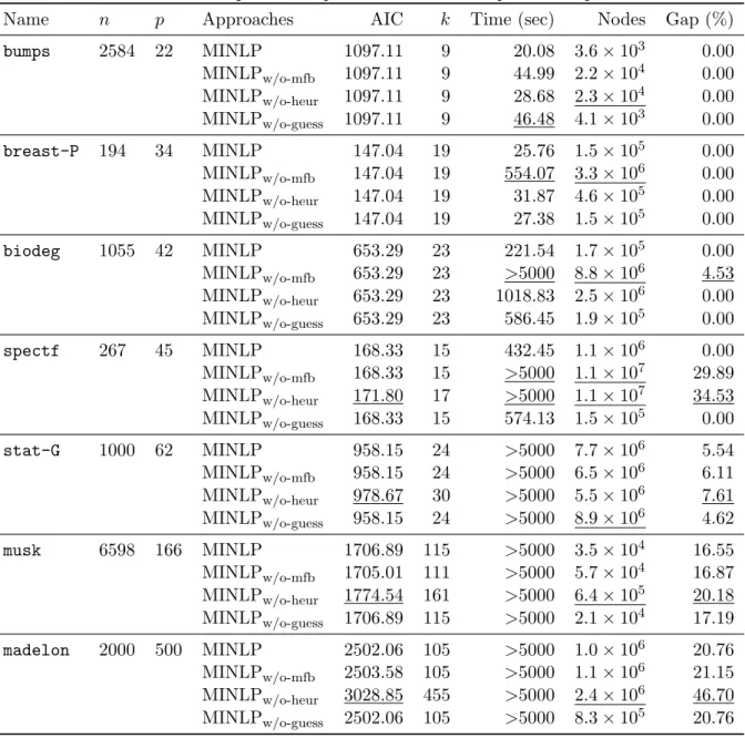
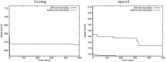
3.4.5 Application 2: Computational performance of developed techniques . . 32
3.4.6 Tables and figures of numerical experiments . . . 34
3.5 Appendix . . . 40
4 Shortest Vector Problem 42 4.1 Overview . . . 42
4.2 Customized branch-and-bound algorithm . . . 43
4.2.1 Computation of bounds on variables . . . 43
4.2.2 Branching . . . 44
4.2.3 Relaxation . . . 45
4.2.4 Heuristic method . . . 47
4.3 IQP approaches using optimization software . . . 48
4.3.1 Convex 0 - 1 IQP approach . . . 48
4.3.2 Partitioning approach . . . 49
4.4 Numerical experiments . . . 51
5 Conclusion 54
Introduction
1.1 Mixed integer nonlinear programming
Mixed integer nonlinear programming (MINLP) can deal with integer variables and nonlin- ear functions and is the most flexible optimization from the viewpoint of formulation. Such optimization problems arise in many real world applications. However, this flexibility leads to numerical difficulties associated with the handling of nonlinear functions and challenges pertaining to optimization in the context of integrality. Nonetheless, many researchers and practitioners have shown interest in solving MINLP problems.
MINLP problems generally form a class of challenging optimization problems because they combine the difficulty of optimizing over integer variables with the handling of nonlinear func- tions. Even though an MINLP problem contains only linear functions, it becomes a mixed integer linear programming (MILP) problem, which is NP-hard [29]. In this study, we deal with convex MINLP problems, which contain convex functions in the objective function and the constraints. A convex MINLP problem are still NP-hard because it contains an MILP problem as a special case. Nevertheless, a convex MINLP problem can be solved much more efficiently than a general MINLP problem.
Several algorithms have been proposed for solving MINLP problems, for example, branch- and-bound algorithm, branch-and-cut algorithm, outer approximation, and Benders decom- position. See [15, 43, 56] for details about these algorithms. In this study, we employ a branch-and-bound algorithm. The idea of this algorithm is to successively divide a given problem into smaller subproblems until each of the subproblems is solvable. This algorithm is widely used to solve optimization problems, and it consists of some components, such as relaxation, branching, heuristics, and presolve. Chapter 2 summarizes this algorithm.
The availability and maturity of software for solving MINLP problems have increased sig- nificantly in the past 20 years. A number of open sources and commercial MINLP solvers are listed in [24]. Notably, state-of-the-art solvers, such as CPLEX [4], Gurobi [3], and FICO Xpress-Optimizer [1], are widely used. These are available for many optimization problems, for example, MILP, mixed integer quadratic programming (MIQP), and mixed integer second- order cone programming (MISOCP) problems. In other words, it is regarded as general-purpose optimization software. In this study, to examine computational performance of our branch- and-bound algorithms, we compare them with conventional algorithms employing CPLEX.
A customized MINLP solver for a specific application occasionally achieves good compu- tational performance [21, 27]. In Chapter 3, we implement a few proposed techniques of a
branch-and-bound algorithm by customizing the SCIP Optimization Suite [5]. This software toolbox comprises several parts, such as SCIP [9, 56] and UG [7]. SCIP is open source software, and it provides a branch-and-bound framework for solving MILP and MINLP problems. Addi- tional plugins, such as branching rules, relaxation handlers, and heuristic methods, allow for an efficient solution process. UG provides a parallel extension of SCIP to employ multi-threaded parallel computation. These software applications have been developed by the Optimization Department at the Zuse Institute Berlin and its collaborators.
1.2 Variable selection
Finding the best statistical model for a given dataset is one of the most important problems in statistical applications (e.g., linear and logistic regression). This problem is calledvariable selection,and solving it leads to the following benefits: improvement in the prediction perfor- mance of a statistical model, development of faster and more cost-effective models in terms of computation, and better understanding of the essence of the statistical model behind a given dataset.
Methods for variable selection are essentially grouped into three methods: filter, wrap- per, and embedded methods. Filter methods select subsets of variables independently to each other. For example, Torkkola [54] proposed a filter method using a mutual information crite- rion. The greatest advantage of filter methods is effective in computational time. However, filter methods tend to select redundant variables because they do not consider the relation- ships between variables. Hence, they are mainly employed as a pre-processing step. Wrapper methods, such as stepwise methods with forward selection and backward elimination, evaluate subsets of variables and consider the interaction between variables. The stepwise methods are implemented in standard statistical software (e.g., R [53]). In each step, the stepwise methods decide whether to add one variable to a statistical model or to remove it and evaluate the statistical model comprised of the selected variables. This process is repeated until no further improvement is possible. Although the stepwise methods are considered greedy algorithms, they often find good statistical models within a short time. Each embedded method performs its particular process and provides good statistical models as a result of the process, for ex- ample, ℓ1-penalized regularization, and decision tree learning. See [31] for more details about variable selection.
In Chapter 3, we focus on direct objective optimization, which is a family of embedded methods. An objective function typically consists of two competing terms: the goodness-of-fit and the number of variables. For example, the Akaike information criterion (AIC) [12] and Bayesian information criterion (BIC) [50] are of the form of such an objective function. Direct objective optimization computes the best subsets of variables in terms of a given objective function. However, computation of all candidates is impractical because the number of them is exponentially large. Notably, most direct objective optimization under linear regression is known to be NP-hard [33].
Showing numerical experiments pertaining to linear and logistic regression, we briefly in- troduce work related to direct objective optimization for them as follows. ℓ1-penalized linear and logistic regression [35, 41] is often employed because it provides sparse models and per- forms well even on large-scale instances. However, the models provided by this approach are not necessarily the best in terms of goodness-of-fit measures. Miyashiro and Takano proposed an MISOCP approach for variable selection based on some information criteria in linear re-
gression [47]. This approach formulate the variable selection as an MISOCP problem, and standard optimization software such as CPLEX [4] and Gurobi [3], are available for the MIS- OCP problem. Bertsimas et al. [17] presented an MILP approach for variable selection in linear regression and developed a discrete extension of modern first order continuous optimiza- tion methods to find high quality feasible solutions. They used the feasible solutions as warm starts of optimization software. Sato et al. [48] formulated an MILP problem by employing a piecewise linear approximation to minimize goodness-of-fit measures for logistic regression.
Although this approach might not arrive at the best logistic model, the results of their compu- tational experiments indicated that this approach outperformed stepwise methods. Bertsimas and King [16] proposed an MINLP approach to constructing logistic models with the desired properties, for example, predictive power, interpretability, and sparsity. In addition, they pro- posed a tailored methodology using outer approximation techniques and dynamic constraint generation to solve the MINLP problem. The risk score problem [55] was optimized for feature selection, integer coefficient, and operational constraints. This problem was formulated as an MINLP problem that can be solved by using the cutting plane algorithm proposed in [55].
1.3 Shortest vector problem
Ann-dimensional lattice is the set of all integral linear combinations ofnlinearly independent vectors in Rn. Lattices have been known in number theory since the eighteenth century, and they already appeared when Lagrange, Gauss, and Hermite studied quadratic forms.
Nowadays, lattices are widely used in the field of cryptology. One of the main problems in lattices is the shortest vector problem (SVP), which is searching for the shortest non-zero vector in a given lattice. SVP is known to be NP-hard under randomized reductions [11]. The security of lattice-based cryptosystems is based on the hardness of SVPs.
The fastest algorithm for solving SVP is the enumeration algorithm presented by Kan- nan [34] and by Fincke and Pohst [28]. Kannan’s algorithm solves SVP in 2O(nlogn), wheren is the lattice dimension. The variant used mostly in practice was presented by Schnorr and Euchner [49]. However, this algorithm also runs in exponential runtime. Roughly speaking, these enumeration algorithms perform a depth first search in a search tree that contains all vectors in a certain search space. So far, enumeration algorithms is applicable to SVPs with low dimensional lattice (n ≲ 60). See the recent work of [25, 32] for details about limita- tions. To gain speed-up, this enumeration algorithm was parallelized [25, 32]. These parallel enumeration algorithms were faster than the then best public implementation.
The LLL algorithm [44] is the first algorithm with a polynomial runtime, although this algorithm searches for shorter vectors rather than the shortest vector. The LLL algorithm can be run in lattice dimensionnup to 1000. In practice, the most promising algorithm for SVPs with high dimensional lattice is the BKZ algorithm [49], which mainly consists of two parts:
an enumeration algorithm in low dimension and the LLL algorithm in high dimension. The BKZ algorithm finds shorter vectors than LLL algorithm and needs higher computational time.
The LLL and BKZ algorithms transform a given lattice to a tractable lattice which consists of shorter basis. Enumeration algorithms is always executed on lattices to which either the LLL or BKZ algorithm is applied in a preprocessing step because these algorithms reduce the runtime significantly compared to the original lattice. The LLL and BKZ algorithms have been improved since these are developed (see, e.g., [46, 52]). The fplll [2] library includes algorithms to search for the shortest or shorter vectors, for example, the LLL, BKZ, and
Kannan’s algorithm.
1.4 Contribution
Standard optimization software is convenient because of availability for many types of opti- mization problems (e.g., MILP and MIQP problems). In fact, state-of-the-art software, such as CPLEX [4] and Gurobi [3], is often used by many researchers and practitioners. Formulating a practical problem as an optimization problem which optimization software can handle, is one of the approaches to solving practical problems. Notably, state-of-the-art software provides good computational performance for MILP problems. However, a practical problem cannot always be formulated as an MILP problem. Even if an MINLP problem is reformulated as an MILP problem, the MILP problem may be poorly designed, and we may not achieve good computational performance. Generally, the computational costs of MINLP problems are much higher than that of MILP problems even though state-of-the-art software is employed. One of the techniques for solving MINLP problems is taking advantage of properties unique to a given optimization problem. Unfortunately, most optimization software does not make use of every such property because it is for solving general optimization problems, such as MILP, MIQP, and MISOCP problems. On the other hand, a customized MINLP solver for a specific problem occasionally achieves good computational performance by using properties and the structure of problems (see, e.g., [21, 27]).
Herein, we focus on two kinds of problems: variable selection and shortest vector problems.
We propose an effective branch-and-bound algorithm for each of the problems. A branch-and- bound algorithm consists of some components, such as relaxation, branching, and heuristic methods. We take advantage of the structure and properties of the problems to improve these components in terms of computational performance. The results of computational experiments show how the proposed algorithms outperform state-of-the-art optimization software.
In Chapter 3, we focus on direct objective optimization in variable selection and formulate it as an MINLP problem. To solve the MINLP problem, we propose an effective branch- and-bound algorithm with a few techniques, for example, cost-effective relaxation, a heuristic method based on stepwise methods, and branching rules. These techniques are based on our previous papers [36, 37, 38]. We show that applications of the formulated MINLP problem include AIC-based variable selection in linear and logistic regression. Therefore, the proposed branch-and-bound algorithm can be applied to these applications. In numerical experiments pertaining to these applications, we show that, for small-scale and medium-scale instances, our solver is faster than conventional approaches using state-of-the-art optimization software. Con- versely, for large-scale instances, our solver find better solutions compared to other approaches even if it cannot determine the optimal value within a realistic time.
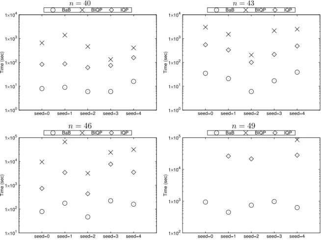
In Chapter 4, we examine how large SVPs can be solved by applying integer quadratic programming (IQP). To this end, we propose an effective branch-and-bound algorithm for SVPs. This algorithm consists of presolve, branching, relaxation, and a heuristic method.
In [40], we proposed the presolve to compute upper and lower bounds on variables. Herein, we propose the other components purpose-built for SVPs. In addition, we propose two convex IQP approaches using high standard optimization software (e.g., CPLEX [4]). We compare the proposed branch-and-bound algorithm with the two convex IQP approaches and shows that the branch-and-bound outperforms the other in terms of computational time.
The remainder of this paper is organized as follows. Chapter 2 presents some basic knowl-
edge about MINLP: the definition of a MINLP problem, special cases related to this study, a branch-and-bound algorithm, and components of it. We discuss direct objective optimization (Chapter 3) and SVP (Chapter 4), respectively, and each of the chapters gives the overview in the first section. We summarize our conclusions in Chapter 5.
Branch-and-Bound Algorithm
2.1 MINLP problems
This section presents the definition of an MINLP problem and special cases related to this study. The MINLP problem is expressed in the following form:
minx f(x)
s.t. x= (x1, . . . , xn)T ∈X, xi ∈Z (i∈I). (MINLP) The set X is a subset of Rn, for example, X = {x ∈ Rn : gj(x) ≤ 0 for all j = 1, . . . , m}. Then,gj(x)≤0 is called aconstraint. The functionf :X →Ris called theobjective function.
The variables x1, . . . , xn contain the integer variables xi (i∈I) and the continuous variables xi (i ∈ {1, . . . , n} \I). If x satisfies x ∈ X and xi ∈ Z for all i ∈ I, x is said to be feasible for (MINLP) or a feasible solution. Otherwise, x is said to be infeasible for it. The purpose of (MINLP) is to find an optimal solution x∗ such that f(x∗) ≤f(x) for any feasible solution x and to compute the optimal value f(x∗). If no feasible solution exists, (MINLP) is said to beinfeasible. Otherwise, (MINLP) is said to be feasible. For convenience, we assume that the objective function f :X →Ris bounded below if (MINLP) is feasible. In this paper, we may denote (MINLP) by
f(x∗) := min
x {f(x) :x∈X, xi ∈Z(i∈I)}.
There exists several special cases of MINLP. Herein, we briefly introduce ones related to this study as follows:
• MILP: If the objective functionf is linear, and (MINLP) contains only linear constraints (i.e., the functionsgj appearing in X are linear), then it is regarded as a mixed integer linear programming (MILP) problem.
• NLP: If all integer constraints xi ∈ Z are removed from (MINLP), it is consider as a nonlinear programming (NLP)problem. Then, the optimal value of the problem without the integer constraints is a lower bound of the optimal value of the original problem.
• convex MINLP: Iff and allgj appearing in X are convex, which means they satisfy the inequality
h(αx+βy)≤αh(x) +βh(y),
whereh ∈ {f, g1, . . . , gm}, and α, β ∈R with α+β = 1 and α, β ≥0, then (MINLP) is called aconvex MINLP problem. Convexity leads to many benefits to solve optimization problems (see e.g., [18, 20]).
• MIQP and IQP: Iff(x) = xTQx+pTx+r, is a (convex) quadratic function ofx, and there are only linear constraints on (MINLP), then it is known as a(convex) mixed integer quadratic programming (MIQP) problem. In addition, if all xj are integer variables, (MINLP) is a (convex) integer quadratic programming (IQP) problem.
• MISOCP: If the objective function is linear, and all nonlinear constraints consist of the form∥Ax+b∥2−cTx≤d, then (MINLP) is amixed integer second-order cone programming (MISOCP)problem.
2.2 Algorithm design
A branch-and-bound algorithm [8, 9, 15, 56] is a design paradigm for discrete and combinatorial optimization problems including (MINLP). The idea of this algorithm is to successively divide a given problem into smaller subproblems until each of the subproblems is solvable. A branch- and-bound algorithm for solving MILP problems was first proposed in [42]. Afterward, Dakin extended the branch-and-bound algorithm to MINLP problems [26]. Other early work related to branch-and-bound algorithms for solving MINLP problems include [19, 30]. All of the most successful optimization software is based on branch-and-bound algorithms or branch-and-cut algorithms [56] which employs cutting planes to tighten the set of feasible solutions. In this section, we briefly introduce a branch-and-bound algorithm. LetP(X) be the problem (MINLP) andθ(X) the optimal value of (MINLP).
Branching: The branch-and-bound algorithm splits repeatedly a set of feasible solutions into a few sets by branching, for example, X = X1∪X2 (X1 ∩X2 = ∅), and constructs a branch-and-bound tree of the nodes corresponding to the split sets. The problemsP(Xj) for both j = 1,2 are called subproblems of P(X). Then, the optimal value θ(X) of P(X) is min{θ(X1), θ(X2)}.
Relaxation: For any nonempty subset Y ⊆ X, a lower bound of the optimal value of subproblem P(Y) is computed by relaxation. By relaxing the integrality of xi (i ∈ I), a standardrelaxation problem to obtain the lower boundℓ(Y) is formulated as follows:
ℓ(Y) := min
x {f(x) :x∈Y}. (2.2.1)
Let R(Y) be the problem (2.2.1). The optimal value ℓ(Y) of R(Y) is a lower bound of θ(Y) because the optimal solution ofP(Y) is feasible forR(Y).
Pruning: Given any feasible solution ¯x of P(X), the branch-and-bound algorithm tests whether nodes can be pruned from the tree. For example, if ℓ(X1) ≥ f(¯x), then θ(X) = min{f(¯x), θ(X2)} because of θ(X) = min{θ(X1), θ(X2)}. Hence, it is not necessary to solve the subproblem P(X1), and the node corresponding X1 can be pruned from the branch-and- bound tree. Feasible solutions are obtained by two procedure. The first one is solving the relaxation problem R(Y). The optimal solution of R(Y) is possibly feasible for P(Y). The second one is a heuristic method (e.g., local search).
In this way, the branch-and-bounds algorithm repeats the branching, relaxation, and prun- ing. We summarize this process in Algorithm 1.
Algorithm 1:Branch-and-bound algorithm Input: An MINLP problem P(X)
Output: An optimal solutionx∗ and the optimal value θ(X) ofP(X) N ← {X} and θ∗ ← ∞;
while N ̸=∅ do
SelectY ∈ N and N ← N \ {Y};
Compute a lower bound ℓof θ(Y) by relaxation;
if ℓ≥θ∗ then continue;
Apply a heuristic method optionally and let ¯x be a feasible solution;
if f(¯x)≤θ∗ thenθ∗ ←x¯ andx∗←x;¯
SplitY into a few subsetsY1, . . . , Yk ⊆Y and N ← N ∪ {Y1, . . . , Yk};
end
θ(X)←θ∗;
return x∗ and θ(X);
2.3 Basic components
In this section, we describe the following basic components of the branch-and-bound algorithm:
relaxation, branching (rules), and heuristic methods. Moreover, we briefly introduce the func- tions of them and techniques.
Relaxation: One of the keys to algorithmic speedup is pruning. To this end, it is necessary to obtain good lower bounds of the optimal values of subproblems. Generally, the standard relaxation problem (2.2.1) is employed to compute a lower bound. Using the structure of a given problem, we may define another relaxation problem. If the optimal value of it is better than that of the standard relaxation problem, it is effective in pruning. For example, Buchheim et al. proposed effective relaxation, which provides better lower bounds for convex IQP problems [23]. There exist other procedures using cutting planes which reduce the sets of feasible solutions of subproblems (see, e.g., [8, Chapter 8]).
We need to consider computational costs of solving relaxation problem because most branch-and-bound algorithms spend much computational time on solving them. For exam- ple, we transformed a standard relaxation problem from a nonconvex NLP problem into a convex quadratic programming problem [38]. Though the nonconvex NLP problem was im- practical, the transformed relaxation problem can be solved with a linear system.
Branching (rules): Most branch-and-bound algorithms employ the branching that uses an optimal solution ˜xof a standard relaxation problemR(Y) and splits a set of feasible solutions into two sets. For any subproblem P(Y), this standard branching selects an indexj ∈I with a fractional value ˜xj and splitsY intoY1 ={x∈Y :xj ≤ ⌊x˜j⌋} andY2 ={x∈Y :xj ≥ ⌈x˜j⌉}. A branching rule is the function for selection of index. Because branching is one of the cores of a branch-and-bound algorithm, it is important for solving MINLP problems to employ good branch rules. In [8, Chapter 5], many branching rules are listed and compared.
Heuristic methods: To prune branch-and-bound nodes from the tree, it is necessary to find good feasible solutions early. Most optimization software contain many heuristic methods for general optimization problems, such as MILP and MIQP problems. However, these methods do not always find feasible solutions. In that case, we should build heuristic methods using the structure of the problem.
Direct Objective Optimization in Variable Selection
3.1 Overview
An objective function of variable selection typically consists of two competing terms (see, e.g., [31]): the goodness-of-fit and the number of explanatory variables. Given a dataset and a statistical model with p parameters, variable selection with this objective function can be formulated as the following MINLP problem:
minβ,z f(β) +λ
∑p j=1
zj (3.1.1)
s.t. zj = 0⇒βj = 0 (j= 1, . . . , p), (3.1.2) βj ∈R, zj ∈ {0,1} (j= 1, . . . , p), (3.1.3) where β = (β1, . . . , βp)T represents the parameters in the given statistical model, and λ is a positive constant. The first term f(β) of the objective function (3.1.1) corresponds to a goodness-of-fit, for example, a discrepancy between the given dataset and the statistical model.
The second termλ∑p
j=1zj operates as a penalty for the number of variables. The constraints (3.1.2) represent indicator constraints, that is, βj has to be zero if zj is zero. This problem (3.1.1)–(3.1.3) is considered asℓ0-penalized variable selection.
We assume the following forf(β) in the objective function (3.1.1):
Assumption 1. For any nonempty subset S ⊆ {1, . . . , p}, we can compute the optimal value and an optimal solution of the following optimization problem:
βmin∈Rp f(β) s.t. βj = 0 (j∈ {1, . . . , p}\S). (3.1.4) Iff is a strongly convex function, the problem (3.1.4) becomes an unconstrained convex prob- lem that can be solved by applying a gradient algorithm, for instance, the steepest descent method and Newton’s method.
In this chapter, we focus on the MINLP problem (3.1.1)–(3.1.3) for variable selection. In Section 3.2, we develop an effective branch-and-bound algorithm to solve (3.1.1)–(3.1.3). This algorithm consists of the following techniques:
(Section 3.2.1) effective relaxation to compute lower bounds, (Section 3.2.2) a heuristic method to find good feasible solutions, (Section 3.2.3) most frequent branching and strong branching.
In Section 3.3, we explain the following applications of the MINLP problem (3.1.1)–(3.1.3):
(Section 3.3.1) AIC minimization for linear regression, (Section 3.3.2) AIC minimization for logistic regression.
In other words, these minimization can be formulated as the form of (3.1.1)–(3.1.3). In Sec- tion 3.4, we show numerical experiments pertaining to AIC minimization for linear and logistic regression and compare the branch-and-bound algorithm developed in Section 3.2 with other approaches. Moreover, we compare the computational performance of the branching rules and examine which of the proposed techniques is effective.
3.2 Customized branch-and-bound algorithm
In [38, 36], we formulated AIC minimization for linear and logistic regression as MINLP prob- lems and proposed branch-and-bound algorithms purpose-built for these problem. These algo- rithms consist of components related to effective relaxation, a heuristic method, and branching rules. In this subsection, we explain how these components are applicable to the MINLP problem (3.1.1)–(3.1.3). In Section 3.2.1, we explain the relaxation to compute lower bounds efficiently. Moreover, we show that a feasible solution of the subproblem can be obtained easily from an optimal solution of the proposed relaxation problem. In Sections 3.2.2, we describe the heuristic method based on stepwise method to find feasible solutions. In Sections 3.2.3, we explain most frequent branching proposed previously [38] and describe strong branching.
3.2.1 Relaxation
Branching fixes a binary variablezj of the problem (3.1.1)–(3.1.3) to zero or one and generates two nodes repeatedly. For any node, we define the setsZ0, Z1, and Z as follows:
Z1 ={j∈ {1, . . . , p}:zj is already fixed to 1}, Z0 ={j∈ {1, . . . , p}:zj is already fixed to 0},
Z ={j∈ {1, . . . , p}:zj is not fixed}.
Then, the subproblem of the problem (3.1.1)–(3.1.3) can be expressed as follows:
minβ,z f(β) +λ
∑p j=1
zj (3.2.1)
s.t. βj ∈R, zj = 1 (j∈Z1), βj =zj = 0 (j∈Z0), (3.2.2) zj = 0⇒βj = 0, βj ∈R, zj ∈ {0,1} (j∈Z). (3.2.3) We denote the subproblem (3.2.1)–(3.2.3) by Q(Z1, Z0, Z) because the subproblem can be specified uniquely by using Z1, Z0,and Z. By relaxing the integrality of the variables zj, we
obtain the following standard relaxation problem ofQ(Z1, Z0, Z):
minβ,z f(β) +λ
∑p j=1
zj (3.2.4)
s.t. βj ∈R, zj = 1 (j∈Z1), βj =zj = 0 (j∈Z0), (3.2.5) zj = 0⇒βj = 0, βj ∈R, 0≤zj ≤1 (j∈Z). (3.2.6) The optimal value of the problem (3.2.4)–(3.2.6) is the lower bound of the optimal value of Q(Z1, Z0, Z). Instead of solving (3.2.4)–(3.2.6), we consider the following problem:
minβ f(β) +λ#(Z1) s.t.βj = 0 (j∈Z0), βj ∈R(j ∈Z1∪Z), (3.2.7) where #(Z1) stands for the number of elements in the set Z1. This problem is arrived at by eliminating the indicator constraints and the variableszj from the problem (3.2.4)–(3.2.6).
Notably, the optimal value of the problem (3.2.7) is the lower bound of the optimal value of Q(Z1, Z0, Z). In fact, the optimal value of (3.2.7) is smaller than or equal to the optimal value of (3.2.4)–(3.2.6) because any feasible solution (β, z) of (3.2.4)–(3.2.6) is also feasible for (3.2.7) and satisfies the following inequality:
f(β) +λ
∑p j=1
zj =f(β) +λ
∑
j∈Z
zj + #(Z1)
≥f(β) +λ#(Z1).
Hence, we employ (3.2.7) as a relaxation problem of the subproblemQ(Z1, Z0, Z) to compute a lower bound of the optimal value ofQ(Z1, Z0, Z). We denote the relaxation problem (3.2.7) byR(Z1, Z0, Z), which is an unconstrained convex problem. We can solveR(Z1, Z0, Z) under Assumption 1.
The following lemma implies that the optimal value of R(Z1, Z0, Z) is identical to the optimal value of the standard relaxation problem (3.2.4)–(3.2.6).
Lemma 3.2.1. Letθ∗ be the optimal value ofR(Z1, Z0, Z). Then, the optimal value of (3.2.4)–
(3.2.6) is θ∗.
Proof. Let β∗ be an optimal solution of R(Z1, Z0, Z). We construct a sequence {(βN, zN)}∞N as follows:
βN =β∗ and zjN =
1 ifj∈Z1, 1/N ifj∈Z, 0 otherwise,
(j= 1, . . . , p)
for all N ≥ 1. (βN, zN) is feasible for (3.2.4)–(3.2.6) for all N ≥ 1. It is sufficient to prove that the objective valueθN of (3.2.4)–(3.2.6) at (βN, zN) converges to the optimal value θ∗ of R(Z1, Z0, Z) as N approaches infinity. Because we haveθ∗ =f(β∗) +λ#(Z1) and
θ∗ ≤θN =f(β∗) +λ#(Z1) + λ
N#(Z) =θ∗+ λ N#(Z),
θN converges to θ∗ as N approaches to infinity. This implies that the optimal value of R(Z1, Z0, Z) is identical to the optimal value of (3.2.4)–(3.2.6).
We can easily solve the relaxation problem of the subproblem obtained by fixing zj to 1.
By fixing the variablezk, two subproblemsQ(Z1∪ {k}, Z0, Z\{k}) andQ(Z1, Z0∪ {k}, Z\{k}) are generated fromQ(Z1, Z0, Z). The relaxation problemR(Z1∪ {k}, Z0, Z\{k}) can then be formulated as follows:
minβ f(β) +λ#(Z1∪ {k}) s.t.βj = 0 (j∈Z0), βj ∈R (Z1∪Z).
Therefore, the optimal value of the relaxation problemR(Z1∪ {k}, Z0, Z\{k}) for any k∈Z isθ∗+λ, whereθ∗ is the optimal value of the relaxation problemR(Z1, Z0, Z).
We explain a procedure to generate a feasible solution of the subproblem Q(Z1, Z0, Z) from an optimal solution of R(Z1, Z0, Z). Let ˆβ = ( ˆβ1, . . . ,βˆp)T be the optimal solution of R(Z1, Z0, Z). We define ˆz = (ˆz1, . . . ,zˆp) by ˆzj = 1 if ˆβj ̸= 0, otherwise ˆzj = 0. Clearly, ( ˆβ,z)ˆ is feasible forQ(Z1, Z0, Z).
3.2.2 Heuristic method based on stepwise methods
To prune shallow nodes from a branch-and-bound tree, it is necessary to find a good feasible solution early. To this end, we develop an effective heuristic method, which is based on stepwise methods with forward selection and backward elimination. The stepwise methods often find good statistical models via goodness-of-fit measures, such as AIC [12] and BIC [50], and these are implemented in statistical software (e.g., R [53]).
First, we briefly explain the stepwise methods. Generally, the stepwise method with forward selection starts with no explanatory variables in a given model and repeats the following steps until no further improvement is possible.
Step 1. Test the addition of each explanatory variable using a chosen goodness-of-fit measure.
Step 2. Add the variable whose inclusion gives the most significant improvement.
The stepwise method with backward elimination starts with all explanatory variables. Instead of adding the variable, it deletes the variable from the model. Although these methods are considered as local search algorithms, they often find good statistical models within a short time.
Next, we extend the capability of the stepwise methods to find feasible solutions of any subproblem Q(Z1, Z0, Z). As a results, we expect that our heuristic methods will find good feasible solutions early. Given any subsetS ⊆ {1, . . . , p} withZ1 ⊆S ⊆Z1∪Z, we define the vector ¯zS = (¯z1S, . . . ,z¯pS)T ∈ {0,1}p as follows:
¯ zjS:=
{
1 ifj∈S
0 ifj∈ {1, . . . , p} \S for all j= 1, . . . , p.
By substituting ¯zS forz inQ(Z1, Z0, Z), it can be rewritten as
βmin∈Rp f(β) +λ#(S) s.t.βj = 0 (j∈ {1, . . . , p} \S), (3.2.8) where #(S) denotes the number of elements inS. An optimal solution of this problem (3.2.8) can be computed under Assumption 1. Let ¯θS and ¯βS be the optimal value and an optimal solution of (3.2.8), respectively. Then, ( ¯βS,z¯S) is a feasible solution of Q(Z1, Z0, Z). In fact,
all the constraints of Q(Z1, Z0, Z) is satisfied because of Z1 ⊆ S ⊆ Z1∪Z and Z0∩S = ∅. Our heuristic method improves repeatedly given feasible solutions by solving problems (3.2.8).
We describe the heuristic method for Q(Z1, Z0, Z) in Algorithm 2. We use ( ¯βZ1,z¯Z1) and ( ¯βZ1∪Z,z¯Z1∪Z) as the initial solutions (β1, z1) and (β2, z2), respectively, in our implementation.
Algorithm 2:Heuristic method based on the stepwise methods
Input: A subproblemQ(Z1, Z0, Z) and two initial feasible solutions (β1, z1) and (β2, z2) ofQ(Z1, Z0, Z)
Output: A feasible solution (β, z) of Q(Z1, Z0, Z) S ←− {j∈ {1, . . . , p}:z1j = 1},vf ←− ∞;
/* the stepwise method with forward selection */
while θ¯S< vf do
vf ←−θ¯S, (βf, zf)←−( ¯βS,z¯S);
Find J = arg min
j∈Z\S
{θ¯S∪{j}: ¯zS∪{j} is feasible forQ(Z1, Z0, Z)}; if J =∅then break;
Selectj ∈J and S ←−S∪ {j}; end
S ←− {j∈ {1, . . . , p}:z2j = 1},vb ←− ∞;
/* the stepwise method with backward elimination */
while θ¯S< vb do
vb←−θ¯S, (βb, zb)←−( ¯βS,z¯S);
Find J = arg min
j∈Z∩S {θ¯S\{j}: ¯zS\{j} is feasible for Q(Z1, Z0, Z)}; if J =∅then break;
Selectj ∈J and S ←−S\ {j}; end
if vf < vb then return(βf, zf);
else return(βb, zb);
3.2.3 Most frequent branching and strong branching
In this section, we customize branching rules to early prune nodes of a branch-and-bound tree. We employ two branching rule: most frequent branchingand strong branching, which are proposed previously [38]. The most frequent branching is based on two tendencies of (3.1.1)–
(3.1.3): a few binary variables zj (j ∈ {1, . . . , p}) of good feasible solutions are often 1, and such variableszj of an optimal solution are 1. The strong branching is based on a branching rule in [8, Section 5.4]. We define this branching suitable for (3.1.1)–(3.1.3).
First, we describe proposed relaxation problems of subproblems generated by branching variable zk. For any subproblem Q(Z1, Z0, Z), if zk (k ∈ Z) is chosen as a branching vari- able, two subproblemsQ(Z1∪ {k}, Z0, Z\{k}) andQ(Z1, Z0∪ {k}, Z\{k}) are generated. The relaxation problems of these subproblems areR(Z1∪ {k}, Z0, Z\{k}), that is,
minβ {f(β) +λ#(Z1∪ {k}) :βj = 0 (j∈Z0), βj ∈R(j = 1, . . . , p)}, (3.2.9)
andR(Z1, Z0∪ {k}, Z\{k}), that is,
minβ {f(β) +λ#(Z1) :βj = 0 (j∈Z0∪ {k}), βj ∈R(j = 1, . . . , p)}. (3.2.10) The optimal value of (3.2.9) isθ∗+λ for anyk∈Z as described in Section 3.2.1, where θ∗ is the optimal value ofR(Z1, Z0, Z). In other words, it does not depends on branching variable whether the corresponding node is pruned from a branch-and-bound tree. Hence, we focus on only the optimal value θ∗k of (3.2.10) for all k ∈Z. To prune the corresponding nodes early, we need to select a branching variable zk (k∈Z) with as large value θk∗ as possible.
Strong branching [8, Section 5.4] tests which of the candidates of branching variable give the best progress in the lower bounds before actually branching on any of them. This test is done by temporarily branching and solving relaxation problems. Applying this strong branching to (3.1.1)–(3.1.3), we execute Algorithm 3. Because this rule means selecting the locally best branching variable, it is generally very effective in terms of the number of subproblems needed to solve the original problem. Unfortunately, the computation time per subproblem of the strong branching are expensive since it is necessary to solve a number of relaxation problems.
Algorithm 3:Strong branching
Input: A set Z of indices of unfixed variables Output: A branching variablezk (k∈Z) forj ∈Z do
Solve R(Z1, Z0∪ {j}, Z\{j}) and obtain the optimal valueθj∗; end
return zk with θk∗= max
j∈Z{θ∗j}
Next, we explain the most frequent branching [38]. When the feasible solution set of a subproblem does not include an optimal solution and good feasible solutions of the original problem, the optimal value of the proposed relaxation problem of the subproblem might be large. As described in the beginning of this subsection, a few binary variableszj of an optimal and good feasible solutions are often 1. Hence, selecting such a variable zk as branching variable, we expect that the optimal value θ∗k of (3.2.10) will be large. We describe this branching rule in Algorithm 4.
Algorithm 4:Most frequent branching
Input: A positive integer N, a setZ of indices of unfixed variables, and the current pool of feasible solutions of (3.1.1)–(3.1.3)
Output: A branching variablezk (k∈Z)
Choose the topN feasible solutions (β1, z1), . . . ,(βN, zN) from the pool;
/* Here (βi, zi) is a feasible solution with the ith lowest objective value
in the pool. */
forj ∈Z do
Compute score valuesj :=
∑N i=1
zji; end
return zk with sk= max
j∈Z{sj}
3.3 Applications
In variable selection, goodness-of-fit measures, for example, AIC [12] and BIC [50], are often employed for evaluation of statistical models. In variable selection based on AIC, the AIC value is computed for each model, and the model with the lowest AIC value is selected as the best statistical model. However, the computation of all candidates is not practical because the number of candidates of possible statistical models is exponentially large. We explain that AIC minimization for linear regression (Section 3.3.1) and logistic regression (Section 3.3.2) can be formulated as the form of the MINLP problem (3.1.1)–(3.1.3). Therefore, applying purpose-built branch-and-bound algorithm described in Section 3.2, we compute efficiently the statistical model with the lowest AIC value. Moreover, we explain techniques for fast implementation in each subsection and Section 3.3.3.
3.3.1 Application 1: AIC minimization for linear regression
We explain that AIC minimization for linear regression can be formulated as the form of the MINLP problem (3.1.1)–(3.1.3) in this subsection. To this end, we define firstly AIC and AIC minimization. Given a dataset withpexplanatory variablesand a statistical model withp+k parameters, the parameter corresponding to thejth explanatory variable is denoted by βj ∈R for allj = 1, . . . , p, and is called acoefficient parameter. If a coefficient parameterβjis nonzero, the statistical model becomes involved with the jth explanatory variable. A statistical model may have parameters except for the coefficient parameters. For instance, a linear regression model has the parameter such as the variance σ2. Let {1, . . . , p} be the set of indices of the given explanatory variables and S a subset of {1, . . . , p}. For any subset S ⊆ {1, . . . , p}, the AIC value of the statistical model with the jth explanatory variables (j ∈ S) is defined as follows:
AIC(S) =−2 max
β {ℓ(β) :βj = 0 (j∈ {1, . . . , p}\S), β∈Rp+k}+ 2(#(S) +k), (3.3.1) whereℓ(β) is the log-likelihood function, and #(S) stands for the number of elements in S. In variable selection based on AIC, the model with the lowest AIC value is selected as the best statistical model. Therefore, this variable selection can be formulated as follows:
minS {AIC(S) :S⊆ {1, . . . , p}}. (3.3.2) This problem (3.3.2) is called AIC minimization. Unfortunately, it is practically difficult to solve (3.3.2) by computing the AIC values of all models because the number of model candidates is 2p.
Secondly, we briefly introduce linear regression. Linear regression is the fundamental sta- tistical tool, and it determines coefficient parametersβ1, . . . , βp ∈R of the following equation from a given dataset:
y=β1+
∑p j=2
βjxj.
Herex2, . . . , xp and yare called explanatory variables and a response variable, respectively. A given dataset is denoted by (xi1, . . . , xip, yi)∈Rp×R (i= 1, . . . , n) withxi1 = 1. Under the
assumption that all the residualϵi =yi−∑p
j=1βjxij are independent and normally distributed with the zero mean and varianceσ2, the log-likelihood function can be formulated as follows:
ℓ(β, σ2) =−n
2log(2πσ2)− 1 2σ2
∑n i=1
yi−
∑p j=1
βjxij
2
. From (3.3.1), the AIC value is computed for anyS⊆ {1, . . . , p}as follows:
AIC(S) =−2 max
β∈Rp,σ2∈R
{ℓ(β, σ2) :βj = 0 (j∈ {1, . . . , p} \S)}
+ 2(#(S) + 1). (3.3.3) We focus on the first term to simplify (3.3.3). By substituting βj = 0 (j ∈ {1, . . . , p} \S) to the objective function, the first term can be regarded as an unconstrained minimization. Thus minimum solutions satisfy the following equation:
dℓ
d(σ2) =− n
2σ2 + 1 2(σ2)2
∑n i=1
yi−
∑p j=1
βjxij
2
= 0.
From this equation, we obtain σ2 = n1∑n
i=1(yi−∑p
j=1βjxij)2. Substituting the variance σ2 to (3.3.3), we simplify (3.3.3) as follows:
AIC(S) = min
β∈Rp
nlog
∑n i=1
yi−
∑p j=1
βjxij
2
: βj = 0 (j∈ {1, . . . , p} \S)
(3.3.4) + 2(#(S) + 1) +n(log(2π/n) + 1).
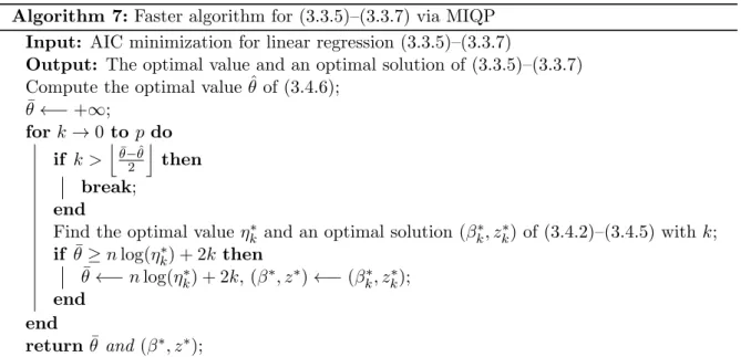
Finally, we formulate the minimization of AIC(S) over S ⊆ {1, . . . , p} as the form of the MINLP problem (3.1.1)–(3.1.3). By eliminating the constant terms of (3.3.4) and introducing auxiliary binary variables z1, . . . , zp ∈ {0,1}, AIC minimization for linear regression can be formulated as follows:
minβ,z nlog
∑n i=1
yi−
∑p j=1
βjxij
2
+ 2
∑p j=1
zj (3.3.5)
s.t. zj = 0⇒βj = 0 (j= 1, . . . , p), (3.3.6) βj ∈R, zj ∈ {0,1} (j= 1, . . . , p), (3.3.7) From (3.2.7), the proposed relaxation problemR(Z1, Z0, Z) of any subproblemQ(Z1, Z0, Z) of (3.3.5)–(3.3.7) can be formulated as follows:
min
β nlog
∑n i=1
yi−
∑p j=1
βjxij
2
+ 2#(Z1) s.t.βj = 0 (j∈Z0), βj ∈R(j= 1, . . . , p). (3.3.8) Although the objective function of (3.3.8) contains the logarithm function, we can freely remove the constant 2#(Z1) and the logarithm by the monotonicity of the logarithm function in (3.3.8), and thus obtain the following problem from (3.3.8):
minβ
∑n i=1
yi−
∑p j=1
βjxij
2
s.t. βj = 0 (j ∈Z0), βj ∈R (j= 1, . . . , p). (3.3.9)
Because the problem (3.3.9) is regarded as the unconstrained minimization of a convex quadratic function, we can compute an optimal solution of (3.3.9) by solving a linear system. Thus Assumption 1 holds for variable selection based on AIC in linear regression. In our imple- mentation, we call dposv function, which is a built-in function of LAPACK [13] for solving the linear system. We denote the optimal value of (3.3.9) byξ∗. The optimal value of (3.3.8) is nlog(ξ∗) + 2#(Z1), and this value is used as a lower bound of the optimal value of the subproblem.
3.3.2 Application 2: AIC minimization for logistic regression
In this section, we formulate AIC minimization for logistic regression as the form of the MINLP problem (3.1.1)–(3.1.3). First, we introduce a logistic regression model. Logistic regression is a fundamental statistical tool, and it estimates the probability of a binary response from a given dataset (xi1, . . . , xip, yi)∈Rp× {0,1}withxi1 = 1 (i= 1, . . . , n). We regardyi as a class label of theith data for all i= 1, . . . , n. Logistic regression determines coefficient parameters β1, . . . , βp of the following logistic regression model which determines the probability of y= 1 for an inputx= (x1, . . . , xp)T ∈Rp,
P(y= 1|x) =
exp(∑p
j=1βjxj
) 1 + exp(∑p
j=1βjxj
).
Here x1, . . . , xp and y are explanatory variables and a response variable, respectively. The probability ofy= 0 is obtained by simple calculation,
P(y= 0|x) = 1−P(y= 1|x) = 1 1 + exp(∑p
j=1βjxj ).
Therefore, the probability ofy∈ {0,1} can be written as
P(y|x) = exp
( y∑p
j=1βjxj ) 1 + exp(∑p
j=1βjxj ).
In logistic regression, the coefficient parameters β1, . . . , βp can be determined by maximum likelihood estimation. In fact, the log-likelihood functionℓis defined as
ℓ(β) =
∑n i=1
logP(yi |xi) =−
∑n i=1
(log(
1 + exp( βTxi))
−yiβTxi) ,
whereβ = (β1, . . . , βp)T and xi = (xi1, . . . , xip)T fori= 1, . . . , n. From (3.3.1), for any subset S⊆ {1, . . . , p}, the AIC value can be computed as follows:
AIC(S) = 2 min
βj
{ n
∑
i=1
(log(
1 + exp( βTxi))
−yiβTxi)
: βj = 0 (j∈ {1, . . . , p} \S) β ∈Rp
}
(3.3.10) + 2#(S).