1. Introduction
Excess comovement among financial asset returns is one of the existing anomalies regarding the covariances between asset returns. Many researchers have challe nged the question of why excess comovement exists among various asset classes and countries using diverse and abundant data sets since Shiller (1989) and Pindyck and Rotemberg (1990). However, the relevant relationship among financial assets remains open to debate.
Theoretically, for example, assuming a Capital Asset Pricing Model (CAPM), the covariance between two assets is expressed by the product of the market betas for each asset and market variance. That means that the relationship between two assets can be completely expressed by a relationship with the market. However, many empirical studies report another factor not theoretically captured in the relationship between two assets. Specifically, empirical evidence has discovered that assets exist in a relationship greater than that indicated by the theory. Pindyck and Rotemberg (1990) call this evidence “excess comovement” and find that
strong excess comovement exists in the U.S. commodity market.
Before discussing the sources of excess comovement, “a certain problem” that occurs when analyzing excess comovement must be reexamined. Many previous papers use residual correlations (or covariances) to determine the existence of excess comovement. Situations in which residual correlations may occur include (1) overlooked factors when calculating the residual series, (2) incorrect formulation for the true structure of the data of interest, and (3) true “excessive” comovement between different assets that researchers require.
The inevitable decision about analyzing excess comove ment is how we define this excessiveness and extract it from the data. For the stock market, fortunately, the theoretical models (e.g., CAPM) for evaluating asset pricing exist. Therefore, though the possibility of (1) and (2) exists, previous studies’ assertion that the model residual series based on a theory is applied to situation (3) seems to have gone thus far uncontested.
* We would like to thank Kohei Aono, Takashi Misumi, Katsuhiko Okada, and Hideaki Kato, participants at the 2012 Association of Behavioral Economics and Finance Meeting, the 2014 Nippon Finance Association Meeting, the 2014 Japanese Economic Association Sprint Meeting, the 2014 Japanese Association of Financial Econometrics and Engineering Summer Meeting and the 2014 Japanese Association of Financial Econometrics and Engineering Winter Meeting. The authors would like to thank Enago (www.enago.jp) for the English language review.
† Musashi University, 1 ‒ 26 ‒ 1, Nerimaku, Toyotama Kami, 167 ‒ 8534, Tokyo, Japan.
in the Japanese stock market
*
Toshifumi Tokunaga
†, Rei Yamamoto
† AbstractWe investigate the monthly excess comovement of three groups categorized by two industry classifications from 1985 to 2013 . Defining excess comovement as a correlation between two stocks beyond what would be justified by the FamaFrench three factor model, we find that 42 % of excess comovement for the group of stocks within the same sectors in the 33 sector classification can be explained by some variables, including the attention measurement, shortterm interest rate, market liquidity, marketwide uncertainty, and information heterogeneity. Results support the hypothesis that excess comovement among stocks within the same sectors correlates positively with the corresponding investor attention.
JEL Classifications: D82, G12, G14
Although early studies concentrated on finding excess comovement among various markets (Pindyck and Rotemberg, 1990, 1993; Karolyi and Stulz, 1996; Deb, Trivedi, and Varangis, 1996), the number of papers analyzing the background has recently been increasing (for the early works, see Barberis and Shleifer, 2003; Barberis, Shleifer, and Wurgler, 2005). Kallberg and Pasquariello (2008) analyze excess comovement using 82 industry indexes in the U.S. stock market to make clear its timeseries characteristics. Defining excess comovement as the squared correlation between two stocks adjusted by fundamental factors, they find that the excess comovement correlates positively to proxies for information heterogeneity and to U.S. monetary and real conditions but correlates negatively to market volatility and the shortterm interest rate.
During the past several years, a research stream has attempted to explain the generating mechanism of excess comovement theoretically by incorporating limited investor attention into a popular basic model. Peng and Xiong (2006) propose a model in which investors have both limited attention in learning about asset fundamentals and overconfidence about their information processing ability. The model describes an investor’s categorylearning behavior of tending to process more market and sector information than firmspecific information. The consequences of limited attention and overconfidence suggest (1) the existence of excess comovement, (2) lower correlations between firms within a sector with a higher informationprocessing efficiency, and (3) correlations weakened over time with the development of information technology. Peng and Xiong (2006) mention that although such phenomena had so far been reported empirically, it seems difficult to explain them using standard rational expectations models.
Mondria (2010) is similar to Peng and Xiong (2006) because both papers are based on Sims’ (2003) rational inattention1. However, Mondria (2010) offers a rational
expectations model of asset prices with information processing constraints, without employing any para
meters expressing investor overconfidence as in Peng and Xiong (2006)2. He suggests that when investors
receive private signals such as linear combinations of two asset returns to update information about two asset returns, changes in one asset affect both asset prices and generate excess comovement by information processing constraints even if returns are essentially uncorrelated.
In contrast, a number of recent studies have docu mented the empirical evidence that limited investor attention affects the timeseries and/or crosssection of asset prices. A great difficulty in analyzing investor attention empirically is how to extract that attention from available data3. Corwin and Coughenour (2008)
measure individual NYSE specialist attention from her portfolio. On the basis of their belief that the attention increases with the number of transaction and absolute return, they analyze how the attention given a stock affects the prices and liquidities of the remaining assigned stocks within her portfolio. Interestingly, the results indicate that even the professional investor is influenced by information processing restrictions. The present study’s main purpose is to evaluate the relationship between limited investor attention and a stock return’s excess comovement at monthly intervals on the basis of daily data. Specifically, we investigate the hypothesis that the information processing capa bility for an investor with limited attention causes excess comovement between two stock returns within the same sectors but not between stocks belonging to different sectors. Hou (2007) finds that the lead lag relations among stock returns are more dominant in an intrasector relationship than in a crosssector relationship. This finding suggests that the information diffusion processes differ between intra and cross sector relationships.
Our hypothesis is based on the idea of transposing “NYSE specialists” and “their remaining assigned stocks,” which were used by Corwin and Coughenour (2008), to “investors” and “other stocks within the same sectors,” respectively. We find that although investors
1 Hirshleifer and Teoh (2003) and Hirshleifer, Lim, and Teoh (2011) model theoretically attention to accounting information. 2 Mondria (2010) refers to two differences from Van Nieuwerburgh and Veldkamp (2009) regarding model assumptions.
3 Mondria, Wu, and Zhang (2010), Da, Engelberg, and Gao (2011), and Garcia (2013) use the search frequency on the Internet as a proxy variable for attention. Mondria and Wu (2010, 2013) and Mondria and QuintanaDomequez (2013) use the quantity of news. Also see Hirshleifer, Hou, Teoh, Zhang (2004) and DellaVigna and Pollet (2007, 2009) for empirical studies.
allocate their attention to their more active stocks during periods of increased activity, they are not as interested in improving prices for other inactive stocks within the same sector. Our result could be interpreted similarly to Mondria (2010), who demonstrates theoretically that when investors receive private signals such as linear combinations of two stock returns, information processing constraints cause excess comovement. In the case of two stocks belonging to different sectors, in contrast, investors seem to have difficulty in receiving any signal from the combination of the two. Therefore, the price change of one stock does not affect the other stock price. As a result, the relationship between the two stocks cannot be easily affected by information processing restrictions.
We find, however, that excess comovement among stocks belonging to different sectors positively correlates to information heterogeneity among investors used by Kallberg and Pasquariello (2008), with no relationship to limited investor attention. This result could be interpreted similarly to Peng and Xiong (2006), who demonstrate theoretically that excess comovement results when overconfident investors concentrate their attention excessively on market information, resulting from lower priority for processing firmspecific infor mation. Therefore, excess comovement between stocks belonging to different sectors correlates to investor categorylearning behavior and overconfidence.
Kallberg and Pasquariello (2008) define excess comove ment as the excess square correlation between two stocks beyond what would be justified by fundamental factors. In contrast, we define it as the correlation between two residual series adjusted by the Fama French three factor model. Moreover, though Kallberg and Pasquariello (2008) calculate weekly excess comove ment by overlapping the data, we calculate monthly excess comovement by not overlapping the data, instead using daily data.
The paper proceeds as follows. In Section 2, we explain how to measure monthly excess comovement. In Section 3, we describe the data and sample characteristics. In Section 4, we present our empirical evidence from the calculations of the various regression models for the Japanese stock market. In Section 5, we conclude the study.
2. Measuring monthly Excess Comovement
When empirically analyzing excess comovement, certain problems should be considered. First, as discussed in the Section 1, excess comovement’s existence depends on the model setting. Fortunately, finance theory offers CAPM, a widely recognized theoretical model explaining financial asset price fluctuation, including comovement. Next, we must decide how to apply the selected model to data. As in previous papers, our choice is usually either to estimate the parameters during the entire sample period, using daily, weekly, or monthly data, or to estimate them by rolling several terms. Although the latter method is adopted for analyzing the time series characteristics of excess comovement, the data overlapping problem should be treated carefully as in Kallberg and Pasquariello (2008).In this study, we define monthly excess comovement using daily individual stock returns to avoid being restricted by the dataoverlapping problem. At month t, we can obtain the monthly comovement between stock
i and stock j by calculating the daily sample correlation
of the OLS residuals from the FamaFrench three factor model as follows: ̂ . 1 ̂ ̂ … (1) where ̂ . 1 ̂ ̂ … (2) ̂ . 1 ̂ ̂ … (3) Where Nt is the number of firms at month t, Dt is the
number of days at month t, ri, d, t is the excess return of
stock i for a riskless return at day d in month t, and, rm, d, t, rSMB, d, t, and rHML, d, t are the market (“market return
minus riskfree rate”), size (“Small minus Big” for market values of firms), and value (“High minus Low” for book tomarket ratios), respectively, in the FamaFrench three factor model. To adjust the skewed distributions of correlations, we apply Fisher’s Z transformation to the correlations: Zij, t = 0.5 × ln (1 + Yij, t) / ln (1 – Yij, t).
Next, we average adjusted excess correlations in a group as follows:
1
… (4) where Sɡ is the set of stocks contained in the ɡth group.
G is the number of the groups, i.e., groups containing
the combinations of two stocks within the same sectors, the combination of two stocks belonging to different sectors, and the combinations of all stocks.
3. Data and Sample Characteristics
A. Data DescriptionTo calculate excess comovement in equation (1), we use the daily return data for all firms listed on the Tokyo Stock Exchange (TSE) First Section from 1987 to 2013. We also calculate daily three factor returns in equation (3), using this data set according to the procedure in Fama and French (1993).
We group the firms listed on the TSE First Section according to two types of sector classifications to test our hypothesis. The first classification comprises 33 sectors based on the subclassification by SICC (Securities Identification Code Committee), which has been used to compose the TSE industry index and is one of the most popular classifications in Japan. The second comprises
six sectors into which we reorganize these 33 groups, referring to the mainclassification (ten groups) by SICC. Table 1 Panel A presents the relationship between the six sectors and the 33 sectors.
This study’s main purpose is to demonstrate that excess comovement between two stocks within the same sector relates to the relative gap of investor attention toward these stocks. Therefore, we determine from the two types of classifications in Panel A whether two firms belong to the same sector. Then, we construct three groups.
The first group consists of all the combinations of two stocks that belong to a same sector in the 33 sector classifications. This group should have a strong connection between stocks. We call a group of such combinations “In33.”
The second group consists of all the combinations of two stocks that belong not only to the same sector in the six sector classifications also to different sectors in the 33 sector classifications. This group should have a weak connection between stocks. We call a group of such combinations “In6 Out33.”
The third group consists of all the combinations of two stocks that belong to different sectors in the six sector classifications. Thus, this group contains all
Table 1: Definition of groups and the number of the sample Panel A. two types of sector classification
Type 1 : 6 sectors Type 2 : 33 sectors (Tokyo Stock Exchange)
HighTechnology Stock Machinery, Electric Appliances, Transportation Equipment, Precision Instruments Cyclical Stock Mining, Textiles & Apparels, Pulp & Paper, Chemicals, Oil & Coal Products,
Rubber Products, Glass & Ceramics Products, Iron & Steel,
Nonferrous Metals, Metal Products, Marine Transportation, Wholesale Trade DomesticDemand Stock Other Products, Land Transportation, Air Transportation,
Warehousing & Harbor Transportation Services, Information & Communication, Retail Trade, Services
Finance & Insurance Banks, Securities & Commodity Futures, Insurance, Other Financing Business Defensive Stock Fishery, Agriculture & Forestry, Foods, Pharmaceutical, Electric Power & Gas Construction & Real Estate Construction, Real Estate
Panel B. the number of combinations: N (N – 1) / 2
Mean Min 1Q Median 3Q Max
All 1,046,425 583,740 759,528 1,003,960 1,389,028 1,546,161
In33 55,626 (5.32%) 30,439 40,142 53,806 74,664 84,026
In6 Out33 163,655 (15.64%) 95,874 117,785 149,279 223,316 253,432
Out6 827,144 (79.04%) 457,427 601,601 800,876 1,090,877 1,208,703
Note: “All” means the group of all the combinations of two stocks among all the stocks. “In33” means the group of all the combinations of two stocks that belong to the same sector in the 33 sector classifications. “In6 Out33” means the group of all the combinations of two stocks that belong not only to the same sector in the six sector classifications but also to different sectors in the 33 sector classifications. “Out6” means the group of all the remaining combinations of two stocks.
the remaining combinations of two stocks. This group should have no connection between stocks. We call a group of such combinations “Out6.”
Table 1 Panel B summarizes the statistics for the number of combinations in each of the four groups at the end of every month. In other words, it is the number of covariances and corresponds to the values N (N – 1) / 2, where N is the number of stocks. On average, approximately 5% of all the combinations of two stocks among all the stocks (“All”) has a strong connection between stocks through sectors, and approximately 15% has a weak connection. If our prediction in Sec tion 1 is supported, our data should show that correlations between excess comovement and attention measurements are strongly significant in the group In33, weak in the group In6 Out33,” and insignificant in the group Out6, even after removing the influence of exogenous variables.
B. Hypothesis
In this study, we prepare proxy variables for investor attention through the following three steps. First, we think that investor attention to each stock relates to the monthly means of daily trading turnover ratios, the monthly standard deviations of daily stock returns, and those products. In other words, our monthly attention based on trading volumes, stock price changes, and those mixtures would contain rich information.
Next, to measure relationships between investor atten tions and return comovements, we define the gap between the attention to the ith stock and the attention to the jth stock as the relative attention between two stocks. Assuming that this attention gap is expanded (i.e., if more attention is allocated to one stock), evaluation of the stock with less attention is neglected or is inappropriately related with the evaluation of another stock with more attention even if both are essentially unrelated. In this study, we think that the latter situation causes excess comovement. For simplicity, this attention gap is called “attention” in the following section.
Finally, to analyze whether excess comovement between two stocks in each group relates to attention gaps, we average the attention gaps for every group. Then, we propose the following hypothesis:
Hypothesis: Excess comovement between two stocks within the same sectors (In33) correlates positively with the corresponding investor attention. In cont rast, excess comovement between two stocks belong ing to different sectors (Out6) is uncorrelated with the corresponding investor attention.
In the situation where investors are exposed to information processing restrictions, Mondria (2010) demonstrates theoretically that investors observing a linear combination of stock returns as a private signal causes excess comovement. Our measurements, such as attention gaps, correlate positively to investor information processing restrictions. However, we predict that although investors observe a linear combination of returns for two stocks within the same sector, they tend to not observe a linear combination of returns for two stocks belonging to different sectors. Probably, a portion of investors for whom trading behavior changes stock price has very few opportunities to investigate stocks belonging to different sectors simultaneously. For example, security analysts usually investigate stocks in a specific sector.
C. Summary Statistics
Our attention measurements are inspired by Corwin and Coughenour (2008), who assert that attention to a given stock increases with trading frequency and absolute return during a period. In their empirical analysis, they arrange the number of trades, the absolute returns, and those products during 30minute intervals based on intraday data. Furthermore, to test the Limited Attention Hypothesis (LAH) that implies a negative relationship between the provision of liquidity for a stock and the level of specialist attention to other stocks in his portfolio, they use a new attention measurement (“PanelAttention”), defined for each stock as the sum of attention across all other stocks by the same specialist panel, excluding the stock of interest. Thus, on the basis of Corwin and Coughenour’s (2008) ideas, we define the three relative attention measures. Table 2 reports summary statistics for excess co move ment and the three attention measures explained in Panel B of Table 1. The categories “attention 1 (A1),” “attention 2 (A2),” and “attention 3 (A3)” denote the logarithm of the absolute value of difference between
two stocks regarding trading turnover ratios, return standard deviations, and those products for stocks within a group, respectively.
Panel A presents the results for the entire combi nation (“All”). Excess comovement follows distribution that has a positive mean and is skewed to the right. Autocorrelations of excess comovement are strongly persistent. The mean and standard deviation of the attention measurement A2 are small relative to those of A1. In other words, A1 and A2 are almost uncorrelated, which suggests that they include certain different information. Autocorrelations of all three attention measures are very strongly persistent. Moreover, excess comovement and three attention measures correlate positively.
Panel B reports the results for the combination of two stocks that belongs to a same sector in the 33 sector classifications (In33). The features of the shape of distribution and the pattern of autocorrelations
resemble those for the entire combination. However, the mean and standard deviation of excess comovement are approximately 10 times larger. Most interestingly, the evidence that excess comovement and the three attention measures are positively correlated, taking no account of influence of other variables, is consistent with the study’s hypothesis.
Panel C reports the results for the combination of two stocks that belong not only to a same sector in the six sector classifications but also to different sectors in the 33 sector classifications (In6 Out33). The features of the shape of distribution and the pattern of autocorrelations are more similar than those of the In33 group to those for the entire combination.
Panel D reports the results for the remaining combi nations of two stocks (Out6). Excess comovement follows a distribution with almost zero mean and a small standard deviation, compared with the other groups. Autocorrelations of excess comovement remain
Table 2: Summary statistics for excess comovement and attention measurements
Mean Median Std. dev. Lag = 1Autocorrelation2 3 correlation correlation correlationwith A1 with A2 with A3 Panel A. All
excess comovement (EC) 0.318 0.273 0.221 0.557 0.467 0.421 0.446 0.269 0.463
attention 1 (A1) –2.183 –2.135 0.602 0.929 0.869 0.821 - 0.016 0.898
attention 2 (A2) –0.476 –0.522 0.281 0.682 0.530 0.445 - - 0.413
attention 3 (A3) –1.429 –1.387 0.612 0.836 0.731 0.662 - - -
Panel B. In33
excess comovement (EC) 3.687 3.564 1.687 0.474 0.353 0.353 0.625 0.055 0.620
attention 1 (A1) –2.322 –2.348 0.613 0.939 0.886 0.844 - –0.009 0.904
attention 2 (A2) –0.554 –0.590 0.269 0.686 0.529 0.448 - - 0.387
attention 3 (A3) –1.571 –1.527 0.632 0.851 0.753 0.691 - - -
Panel C. In6 Out33
excess comovement (EC) 0.858 0.734 0.607 0.413 0.337 0.360 0.500 0.169 0.514
attention 1 (A1) –2.175 –2.125 0.608 0.931 0.873 0.822 - –0.001 0.899
attention 2 (A2) –0.500 –0.539 0.271 0.677 0.518 0.439 - - 0.393
attention 3 (A3) –1.413 –1.356 0.613 0.841 0.739 0.666 - - -
Panel D. Out6
excess comovement (EC) –0.016 –0.026 0.245 0.432 0.376 0.300 –0.059 0.151 –0.047
attention 1 (A1) –2.176 –2.122 0.601 0.928 0.866 0.818 - 0.022 0.898
attention 2 (A2) –0.466 –0.505 0.285 0.683 0.532 0.446 - - 0.419
attention 3 (A3) –1.423 –1.380 0.612 0.833 0.727 0.658 - - -
Note: “All” means the group of all the combination of two stocks among all the stocks. “In33” means the group of all the combinations of two stocks that belong to the same sector in the 33 sector classifications. “In6 Out33” means the group of all the combination of two stocks that belong not only to the same sector in the six sector classifications but also to different sectors in the 33 sector classifications. “Out6” means the group of all the remaining combinations of two stocks. The attention measurement “A1” denotes the series of averaging the logarithm of the absolute value of the difference between two stocks regarding trading turnover ratios for stocks within a group. The attention measurement “A2” denotes the series of averaging the logarithm of the absolute value of the difference between two stocks regarding return standard deviations for stocks within a group. The attention measurement “A3” denotes the series of averaging the logarithm of the absolute value of the difference between two stocks regarding the product of trading turnover ratios and return standard deviations for stocks within a group.
strongly persistent. Interestingly, the evidence that excess comovement and two attention measurements (A1 and A3) are uncorrelated, if taking no account of the influence of other variables, is consistent with the study’s hypothesis.
D. Relationship between Excess Comovement and Attention Measurement
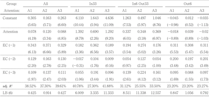
Because excess comovement is strongly persistent as Table 2 reports, it is necessary to evaluate the time series characteristics appropriately. Table 3 reports the results of regressions of excess comovements on attention measurement and excess comovements with three lags. The LjungBox Q tests for autocorrelation in the residual series with six lags (LB (6)) are not significant at the 5% level for all cases, indicating that the time series characteristics of excess comovement are appropriately adjusted by the autoregressive (AR) terms of the dependent variable.
Interestingly, the coefficients of all three attention measures for the group In33 are positive and statistically significant. However, those for the group Out6 are not statistically significant. These results remain consistent with the study’s hypothesis as in Table 2’s results, if taking no account of the influence of other variables. In
Section 4, we discuss the relationship between excess comovement and investor attention using the models described in Table 3 as the basic models.
In empirical analysis, it is important to remove the influence of any common factor likely to affect the relationship between stocks must be removed. We use the following twelve explanatory variables expected to affect an excess comovement identified by Kallberg and Pasquariello (2008).
The variable “monthly market return with dividend” (symbol “Rm”) enables us to measure the effect of market information. The variable “monthly rate of change of yen/ dollar” (symbol “YD”) seems to be an important macro variable because many Japanese firms depend strongly on export. The variables “monthly CD rate (three month) at the end of the month” (symbol “CD”) and “monthly yield spread between tenyear government bond yield and CD rate” (symbol “YS”) relate to the Japanese financial policy. The variables “monthly liquidity measure” (symbol “PS”) and “monthly illiquidity measure” (symbol “IL”) are proposed by Pastor and Stambaugh (2003) and Amihud (2002), respectively. Moreover, the variable “monthly trading value on TSE First Section” (symbol “TV”) is a popular proxy for investors’ trading activity. The variables “bull markets for three months”
Table 3: Time-series regressions of excess comovement on attention measurement with lagged dependent variables (ECs)
Group: All In33 In6 Out33 Out6
Attention: A1 A2 A3 A1 A2 A3 A1 A2 A3 A1 A2 A3 Constant 0.305 0.163 0.263 6.110 1.643 4.636 1.263 0.497 1.046 -0.045 0.012 -0.035 (5.65) (5.71) (6.60) (10.44) (5.94) (11.09) (7.53) (5.97) (8.76) (-0.98) (0.52) (-1.13) Attention 0.078 0.120 0.088 1.392 0.690 1.292 0.337 0.348 0.369 -0.018 0.039 -0.02 (4.19) (3.34) (4.85) (8.79) (2.26) (9.20) (6.01) (3.18) (6.97) (-0.89) (0.89) (-1.03) EC (-1) 0.343 0.371 0.329 0.182 0.362 0.189 0.194 0.274 0.176 0.311 0.308 0.311 (6.13) (6.66) (5.89) (3.36) (6.56) (3.57) (3.54) (5.02) (3.26) (5.53) (5.47) (5.54) EC (-2) 0.129 0.163 0.130 -0.017 0.104 0.009 0.054 0.127 0.054 0.200 0.197 0.201 (2.20) (2.78) (2.25) (-0.31) (1.76) (0.16) (0.97) (2.25) (1.00) (3.48) (3.42) (3.49) EC (-3) 0.109 0.137 0.111 0.055 0.191 0.096 0.139 0.224 0.161 0.095 0.088 0.097 (1.97) (2.47) (2.03) (1.06) (3.44) (1.91) (2.61) (4.12) (3.12) (1.69) (1.55) (1.73) adj. R2 38.52% 37.30% 39.61% 40.78% 27.30% 41.88% 31.12% 25.55% 33.50% 23.20% 23.20% 23.27% LB (6) 0.425 0.914 0.427 6.009 3.335 11.333 8.511 11.338 12.557 0.847 1.056 0.792
Note: “All” means the group of all the combinations of two stocks among all the stocks. “In33” means the group of all the combinations of two stocks that belong to a same sector in the 33 sector classifications. “In6 Out33” means the group of all the combinations of two stocks that belong not only to the same sector in the six sector classifications but also to different sectors in the 33 sector classifications. “Out6” means the group of all the remaining combinations of two stocks. “EC” is excess comovement, and the number in parentheses is a lag of a month’s interval. tstatistics are reported in parentheses. “adj.R2” denotes the coefficient of determination adjusted by the degree of freedom. “LB (6)” denotes the LjungBox Q
Table 4: Correlation matrix of explanatory variables Rm YD CD YS PS IL TV d+ d– σm H1 H2 N Rm 1.00* YD 0.15* 1.00* CD –0.08* –0.05* 1.00* YS 0.04* 0.04* –0.66* 1.00* PS 0.20* 0.00* –0.24* 0.14♦ 1.00* IL –0.15* –0.08* 0.22* 0.06* –0.55* 1.00* TV 0.06* 0.05* –0.10† –0.08* 0.08* –0.17* 1.00* d+ 0.33* 0.09† –0.13♦ 0.01* 0.25* –0.28* 0.09* 1.00* d– –0.38* –0.14♦ 0.02* –0.09† –0.20* 0.20* 0.07* –0.17* 1.00* σm –0.25* –0.16* –0.06* –0.10† –0.35* 0.19* –0.01* –0.14♦ 0.35* 1.00* H1 –0.13♦ –0.05* –0.06* 0.07* –0.08* 0.24* –0.03* –0.05* 0.09* 0.04* 1.00* H2 –0.12♦ –0.08* –0.24* 0.18* –0.15* 0.38* –0.05* –0.08* 0.15* 0.10† 0.73* 1.00* N 0.00* –0.03* –0.65* 0.13♦ 0.08* –0.35* 0.16* 0.12♦ 0.06* 0.11♦ –0.02* 0.22* 1.00*
Note: “Rm” denotes monthly market return with dividend. “YD” denotes monthly rate of change of the yen/dollar. “CD” denotes monthly CD rate (three month) at the end of the month. “YS” denotes monthly yield spread between short—term interest rate and long—term government bond yield at the end of the month. “PS” denotes the liquidity measurement proposed by Pastor and Stambaugh (2003). “IL” denotes the illiquidity measurement proposed by Amihud (2002). “TV” denotes the monthly trading value at TSE 1st floor. Note that “d+” (“d–”) is a dummy variable equal to one if sign (r (m, t) = sign (r(m, t–1) = sign (rm, t–2) = + (–), and zero otherwise, which are the same definitions used by Kallberg and Pasquariello (2008).
Furthermore “σm” is proxy for market uncertainty measured as the monthly standard deviation of daily market returns within the same month. “H1” and “H2” are proxies for the degree of information heterogeneity based on the crosssectional mean of the standard deviations of analysts’ EPS forecasts and ratios of the differences between their highest and lowest forecasts, respectively, which are the same definitions used by Kallberg and Pasquariello (2008). Finally, “N” is the crosssectional mean number of analysts covering the forecasted firms. A “†,” “◆,” or “*”
indicate significance at the 10%, 5%, or 1% level, respectively.
Table 5: Time-series regressions of excess comovement on each explanatory variable
Group: Const. SlopeAll adj. R2 Const. SlopeIn33 adj. R2 Const. In6 Out33Slope adj. R2 Const. SlopeOut6 adj. R2
Rm 0.319 0.003 0.37% 3.676 0.048 2.34% 0.858 0.011 0.69% –0.015 –0.001 –0.23% (25.55) (1.48) (39.11) (2.93) (25.21) (1.79) (–1.08) (–0.51) YD 0.319 0.000 –0.31% 3.682 –0.002 –0.32% 0.859 –0.009 –0.10% –0.015 0.001 –0.30% (25.50) (–0.13) (38.65) (–0.07) (25.14) (–0.82) (–1.09) (0.25) CD 0.389 –0.042 18.67% 3.743 –0.037 –0.07% 0.937 –0.047 2.85% 0.053 –0.041 14.26% (27.97) (–8.58) (31.86) (–0.88) (22.56) (–3.20) (3.33) (–7.32) YS 0.314 0.006 –0.28% 4.106 –0.441 3.94% 0.949 –0.094 1.17% –0.07 0.057 3.04% (15.93) (0.35) (27.98) (–3.74) (17.77) (–2.18) (–3.26) (3.30) PS 0.348 0.610 3.09% 3.882 4.223 2.50% 0.921 1.296 1.74% –0.004 0.232 0.09% (23.13) (3.33) (33.80) (3.01) (22.24) (2.57) (–0.25) (1.13) IL 0.413 –0.072 9.79% 4.796 –0.86 24.25% 1.132 –0.211 11.10% –0.028 0.010 –0.16% (20.91) (–5.94) (34.81) (–10.11) (21.13) (–6.36) (–1.21) (0.70) TV 0.314 0.096 1.17% 3.663 0.390 0.11% 0.850 0.185 0.42% –0.018 0.051 0.03% (24.93) (2.18) (37.96) (1.16) (24.58) (1.53) (–1.26) (1.04) d+ 0.298 0.140 4.73% 3.505 1.201 6.07% 0.819 0.275 2.28% –0.021 0.042 0.05% (22.58) (4.09) (35.09) (4.63) (22.39) (2.89) (–1.42) (1.07) d- 0.324 –0.035 –0.01% 3.760 –0.561 1.00% 0.873 –0.097 –0.01% –0.017 0.012 –0.29% (24.07) (–0.98) (36.88) (–2.05) (23.72) (–0.98) (–1.13) (0.31) σm 0.233 0.071 3.54% 3.085 0.498 2.91% 0.542 0.265 6.75% –0.019 0.003 –0.31% (8.61) (3.55) (14.91) (3.24) (7.44) (4.89) (–0.62) (0.14) H1 0.274 0.416 0.29% 4.329 –5.959 1.84% 1.168 –2.85 3.51% –0.177 1.489 6.09% (7.87) (1.39) (16.46) (–2.63) (12.48) (–3.54) (–4.73) (4.63) H2 0.249 0.220 1.44% 4.655 –3.079 5.61% 1.138 –0.882 3.46% –0.222 0.656 12.49% (7.83) (2.37) (19.61) (–4.45) (13.21) (–3.51) (–6.71) (6.79) N –0.358 0.103 22.56% 0.981 0.412 5.97% –0.401 0.192 10.30% –0.413 0.061 6.16% (–5.04) (9.65) (1.65) (4.59) (–1.92) (6.11) (–4.78) (4.66)
Note: The symbols for the explanatory variables are the same as in Table 4. tstatistics are reported in parentheses. “adj.R2” denotes the coefficient of
and “bear markets for three months” (symbols “d+” and “d–”) are the dummy variables that equal to one if sign (rm, t) = sign (rm, t–1) = sign (rm, t–2) = + (–), and zero
other wise. The variable “market uncertainty” (symbol “σm”) enables us to measure the level of marketwide information asymmetry. We measure this variable as monthly standard deviation of daily market returns within a month. The variables “information heterogeneity” (symbols “H1” and “H2”) enable us to measure the degree of information heterogeneity. We measure these variables as crosssectional means of the standard deviations of analysts’ EPS forecasts and the ratios of the differences between their highest and lowest forecasts, respectively. Finally, the variable “the number of analysts” (symbol “N”) is added to information asymmetry and heterogeneity. We measure this variable as the crosssectional mean number of analysts covering the forecast firms.
Table 4 reports the correlations between variables that are likely to affect excess comovement. Following Kallberg and Pasquariello (2008), “σm,” “H1,” “H2,” and “N” are classified as proxies for information asymmetry and heterogeneity. “CD,” “d+,” and “d-” are classified as proxies for liquidity shocks. These values are utilized for variable selection in a multiple regression model. For example, variables “IL” and “TV” or variables “H1” and “H2” are not simultaneously included in a model. Table 5 reports the estimation results for the time series simple regressions of excess comovement on each explanatory variable. The variable “Rm” is positive and significant for the group In33 but not significant for the group Out6. In other words, market information causes excessive comovement of stocks within the same sectors, even after removing the market factor from individual returns. The variable “YD” does not affect excess comovement.
The variable “CD” can be interpreted in directly oppo site ways, as summarized by Kallberg and Pasquariello. On one hand, the trading activity by financially const rained investors generates the positive correlation between interest rate and excess comovement (Shiller, 1989; Calvo, 1999; Kyle and Xiong, 2001; Yuan, 2005). On the other hand, the portfolio rebalancing activity by cost sensitive investors generates the negative correlation between interest rate and excess comovement (Fleming, Kirby, and Ostdiek, 1998; Kodres and Pritsker, 2002;
Pasquariello, 2007). The results in Table 5 are more consistent with the latter interpretation, as are the results in Kallberg and Pasquariello (2008). The variables “PS,” “IL,” and “TV” can be interpreted similarly to the variable “CD.” Naturally, the relationships with the variable “CD” are expected to be negative for the variables “PS” and “TV” but positive for the variable “IL.” The results reveal that the coefficients of the three variables in the case of the group In33 satisfy the sign conditions. Especially, the coefficients of the variables “PS” and “IL” are strongly significant. The variables “d+” and “d-” enable us to estimate the asymmetric relationship between excess comovement and market conditions. Although Kallberg and Pasquariello (2008) find a positive correlation with excess comovement only in the U.S. bull markets, our results reveal a symmetric relationship for In33 and a nonrelationship for Out6. The variable “σm” can be interpreted in directly opposite ways, as summarized by Kallberg and Pasqu ariello (2008). On one hand, the inability to distinguish between idiosyncratic and systematic shocks derived from greater market uncertainty generates a positive correlation between market volatility and excess comove ment. On the other hand, the improvement in the relative precision of traders’ signals derived from greater market uncertainty generates a negative correlation between market volatility and excess comovement. The result for In33 reported in Table 5 is consistent with the former interpretation, contrary to the results in Kallberg and Pasquariello (2008). However, our results reveal a nonrelationship for Out6. The variables “H1” and “H2” seem to be positively correlated to investors’ cross inference regarding fundamentals. Pasquariello (2007) suggests that if information heterogeneity increases, investors’ crossinference becomes increasingly in correct and causes excess comovement. The results for Out6 demonstrate significantly positive correlations and are consistent with Pasquariello (2007). However, the results for In33 demonstrate significantly negative correlations. The results for the additional variable “N” demonstrate significantly positive correlations.
4. Empirical Results
Our main purpose in this study is to evaluate the relationship between excess comovement and investor attention correctly. In Section 4, we presented two im
por tant results. The first is that the sectors to which the pair of stocks used for measurement of comovement belong exhibit different relationships between excess comovement and investor attention. The second is that excess comovement has a strong relationship with certain exogenous variables.
In this section, we evaluate these results as a whole to support a conclusion regarding our hypothesis. In the second half of this section, we verify that the results do not change, even taken into consideration the influence of size. Finally, focusing on information heterogeneity, we empirically consider the generating mechanism of excess comovement suggested by the theoretical model of Peng and Xiong (2006).
A. Explaining Excess Comovement by Explanatory Variables Related to the Stock Market
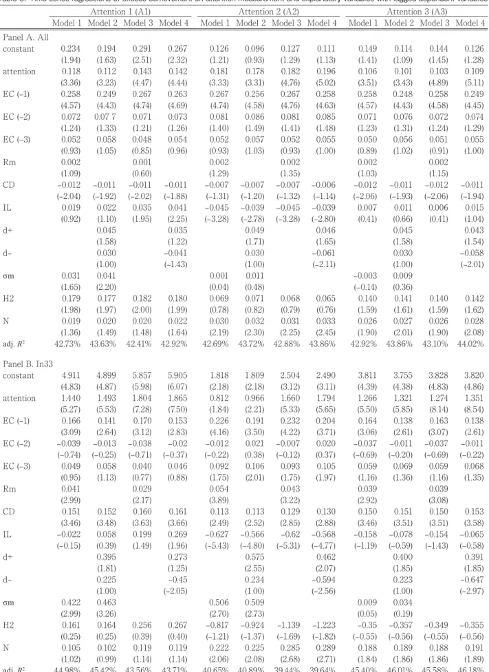
Table 6 reports the results for time series regressions of excess comovement on attention measurement and explanatory variables with lagged dependent variables. The first four explanatory variables reflect the results reported in Table 3. In other words, we take into con sideration that excess comovement is strongly persistent. The remaining explanatory variables reflect the results reported in Table 5. We fix four variables (interest rate (“CD”), liquidity (“IL”), information heterog eneity (“H2”), and the number of analysts (“N”)) that have high explanatory power in the single regressions of the four models. Next, although Model 1 and Model 3 include the market return variable (“Rm”), Model 2 and Model 4 include the market condition variables (“d+” and “d-”) instead of market return. Although Model 1 and Model 2 include market volatility (“σm”), the coefficient of which can be positive and negative, Model 3 and Model 4 do not include it. Panel A presents the results for the entire combination (“All”). The twelve regressions that comprise three attention measures and four regression models demonstrate that all the adjR2s exceed 40%.
Panel B reports the results for the combination of two stocks that belong to a same sector in the 33 sector classifications (In33). The twelve regressions reveal that the adjR2s range from 39.44% to 46.18%. The coefficients
of the variable “attention” are positively significant except in Model 1 for Attention 2, even taking into con sideration the influence of explanatory variables. These results support our hypothesis that excess comovement
among stocks within the same sectors correlates positively with the corresponding investor attention. The coefficients of the variable “Rm” are positively significant as in the single regression results reported in Table 5. The coefficients of the variable “CD” are positively significant in the multiple regressions but are not significant in the single regression. This outcome means that the trading activity by financial constrained investors causes excess comovement. Although the co efficient of the variable “IL” is negatively significant in the single regression, the influence on excess comovement weakens in multiple regressions. The coefficients of the variable “d+” have more stable explanation power than the coefficients of the variable “d–.” This outcome is similar to the results in Kallberg and Pasquariello (2008). It seems, however, that no clear asymmetric reactions occur under the market conditions. The coefficients of the variable “σm” remain positively significant although the influence on excess comovement slightly weakens. The coefficients of the variable “H2” are not significant in the multiple regressions but are negatively significant in the single regression. This outcome means that other variables absorb the influence of information heterogeneity. Although the coefficient of the variable “N” is positively significant in the single regression, the influence on excess comovement weakens in multiple regressions.
In summary, the results of the twelve regressions support our hypothesis. Furthermore, excess comove ment moves together with the market and especially increases with market uncertainty during bull markets. Excess comovement also relates to trading activity by financially constrained investors.
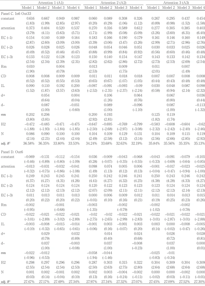
Panel B reports the results for the combination of two stocks that belong not only to the same sector in the six sector classifications but also to different sectors in the 33 sector classifications (In6 Out33). Although these results as a whole resemble those in Panel B, the explanation power of each variable seems weaker, which may be attributed to the weak connections between stocks in this group.
Panel D reports the results for the remaining combination (Out6). The twelve regressions reveal that the adjR2s range from 27.07% to 27.97%. These
outcomes are lower than the values for In33 (Panel B). In other words, few variables have high explanation
Table 6: Time-series regressions of excess comovement on attention measurement and explanatory variables with lagged dependent variables
Attention 1 (A1) Attention 2 (A2) Attention 3 (A3)
Model 1 Model 2 Model 3 Model 4 Model 1 Model 2 Model 3 Model 4 Model 1 Model 2 Model 3 Model 4 Panel A. All constant 0.234 0.194 0.291 0.267 0.126 0.096 0.127 0.111 0.149 0.114 0.144 0.126 (1.94) (1.63) (2.51) (2.32) (1.21) (0.93) (1.29) (1.13) (1.41) (1.09) (1.45) (1.28) attention 0.118 0.112 0.143 0.142 0.181 0.178 0.182 0.196 0.106 0.101 0.103 0.109 (3.36) (3.23) (4.47) (4.44) (3.33) (3.31) (4.76) (5.02) (3.51) (3.43) (4.89) (5.11) EC (–1) 0.258 0.249 0.267 0.263 0.267 0.256 0.267 0.258 0.258 0.248 0.258 0.249 (4.57) (4.43) (4.74) (4.69) (4.74) (4.58) (4.76) (4.63) (4.57) (4.43) (4.58) (4.45) EC (–2) 0.072 0.07 7 0.071 0.073 0.081 0.086 0.081 0.085 0.071 0.076 0.072 0.074 (1.24) (1.33) (1.21) (1.26) (1.40) (1.49) (1.41) (1.48) (1.23) (1.31) (1.24) (1.29) EC (–3) 0.052 0.058 0.048 0.054 0.052 0.057 0.052 0.055 0.050 0.056 0.051 0.055 (0.93) (1.05) (0.85) (0.96) (0.93) (1.03) (0.93) (1.00) (0.89) (1.02) (0.91) (1.00) Rm 0.002 0.001 0.002 0.002 0.002 0.002 (1.09) (0.60) (1.29) (1.35) (1.03) (1.15) CD –0.012 –0.011 –0.011 –0.011 –0.007 –0.007 –0.007 –0.006 –0.012 –0.011 –0.012 –0.011 (–2.04) (–1.92) (–2.02) (–1.88) (–1.31) (–1.20) (–1.32) (–1.14) (–2.06) (–1.93) (–2.06) (–1.94) IL 0.019 0.022 0.035 0.041 –0.045 –0.039 –0.045 –0.039 0.007 0.011 0.006 0.015 (0.92) (1.10) (1.95) (2.25) (–3.28) (–2.78) (–3.28) (–2.80) (0.41) (0.66) (0.41) (1.04) d+ 0.045 0.035 0.049 0.046 0.045 0.043 (1.58) (1.22) (1.71) (1.65) (1.58) (1.54) d– 0.030 –0.041 0.030 –0.061 0.030 –0.058 (1.00) (–1.43) (1.00) (–2.11) (1.00) (–2.01) σm 0.031 0.041 0.001 0.011 –0.003 0.009 (1.65) (2.20) (0.04) (0.48) (–0.14) (0.36) H2 0.179 0.177 0.182 0.180 0.069 0.071 0.068 0.065 0.140 0.141 0.140 0.142 (1.98) (1.97) (2.00) (1.99) (0.78) (0.82) (0.79) (0.76) (1.59) (1.61) (1.59) (1.62) N 0.019 0.020 0.020 0.022 0.030 0.032 0.031 0.033 0.026 0.027 0.026 0.028 (1.36) (1.49) (1.48) (1.64) (2.19) (2.30) (2.25) (2.45) (1.90) (2.01) (1.90) (2.08) adj. R2 42.73% 43.63% 42.41% 42.92% 42.69% 43.72% 42.88% 43.86% 42.92% 43.86% 43.10% 44.02% Panel B. In33 constant 4.911 4.899 5.857 5.905 1.818 1.809 2.504 2.490 3.811 3.755 3.828 3.820 (4.83) (4.87) (5.98) (6.07) (2.18) (2.18) (3.12) (3.11) (4.39) (4.38) (4.83) (4.86) attention 1.440 1.493 1.804 1.865 0.812 0.966 1.660 1.794 1.266 1.321 1.274 1.351 (5.27) (5.53) (7.28) (7.50) (1.84) (2.21) (5.33) (5.65) (5.50) (5.85) (8.14) (8.54) EC (–1) 0.166 0.141 0.170 0.153 0.226 0.191 0.232 0.204 0.164 0.138 0.163 0.138 (3.09) (2.64) (3.12) (2.83) (4.16) (3.50) (4.22) (3.71) (3.06) (2.61) (3.07) (2.61) EC (–2) –0.039 –0.013 –0.038 –0.02 –0.012 0.021 –0.007 0.020 –0.037 –0.011 –0.037 –0.011 (–0.74) (–0.25) (–0.71) (–0.37) (–0.22) (0.38) (–0.12) (0.37) (–0.69) (–0.20) (–0.69) (–0.22) EC (–3) 0.049 0.058 0.040 0.046 0.092 0.106 0.093 0.105 0.059 0.069 0.059 0.068 (0.95) (1.13) (0.77) (0.88) (1.75) (2.01) (1.75) (1.97) (1.16) (1.36) (1.16) (1.35) Rm 0.041 0.029 0.054 0.043 0.039 0.039 (2.99) (2.17) (3.89) (3.22) (2.92) (3.08) CD 0.151 0.152 0.160 0.161 0.113 0.113 0.129 0.130 0.150 0.151 0.150 0.153 (3.46) (3.48) (3.63) (3.66) (2.49) (2.52) (2.85) (2.88) (3.46) (3.51) (3.51) (3.58) IL –0.022 0.058 0.199 0.269 –0.627 –0.566 –0.62 –0.568 –0.158 –0.078 –0.154 –0.065 (–0.15) (0.39) (1.49) (1.96) (–5.43) (–4.80) (–5.31) (–4.77) (–1.19) (–0.59) (–1.43) (–0.58) d+ 0.395 0.273 0.575 0.462 0.400 0.391 (1.81) (1.25) (2.55) (2.07) (1.85) (1.85) d– 0.225 –0.45 0.234 –0.594 0.223 –0.647 (1.00) (–2.05) (1.00) (–2.56) (1.00) (–2.97) σm 0.422 0.463 0.506 0.509 0.009 0.034 (2.99) (3.26) (2.70) (2.73) (0.05) (0.19) H2 0.161 0.164 0.256 0.267 –0.817 –0.924 –1.139 –1.223 –0.35 –0.357 –0.349 –0.355 (0.25) (0.25) (0.39) (0.40) (–1.21) (–1.37) (–1.69) (–1.82) (–0.55) (–0.56) (–0.55) (–0.56) N 0.105 0.102 0.119 0.119 0.222 0.225 0.285 0.289 0.188 0.189 0.188 0.191 (1.02) (0.99) (1.14) (1.14) (2.06) (2.08) (2.68) (2.71) (1.84) (1.86) (1.86) (1.89) adj. R2 44.98% 45.42% 43.56% 43.71% 40.65% 40.89% 39.44% 39.64% 45.40% 46.01% 45.58% 46.18%
Table 6: —Continued
Attention 1 (A1) Attention 2 (A2) Attention 3 (A3)
Model 1 Model 2 Model 3 Model 4 Model 1 Model 2 Model 3 Model 4 Model 1 Model 2 Model 3 Model 4 Panel C. In6 Out33
constant 0.616 0.667 0.949 0.987 0.060 0.089 0.308 0.326 0.267 0.295 0.437 0.454 (1.83) (1.99) (2.85) (2.97) (0.20) (0.29) (1.06) (1.12) (0.89) (0.98) (1.52) (1.58) attention 0.373 0.404 0.520 0.537 0.270 0.316 0.589 0.612 0.277 0.305 0.385 0.403 (3.79) (4.11) (5.63) (5.71) (1.71) (1.99) (5.08) (5.09) (3.26) (3.60) (6.31) (6.40) EC (–1) 0.154 0.140 0.169 0.164 0.183 0.166 0.190 0.179 0.161 0.146 0.160 0.149 (2.87) (2.60) (3.09) (3.00) (3.39) (3.06) (3.47) (3.26) (2.99) (2.71) (2.96) (2.76) EC (–2) 0.026 0.028 0.025 0.026 0.048 0.054 0.046 0.051 0.030 0.033 0.025 0.026 (0.49) (0.52) (0.46) (0.47) (0.88) (0.99) (0.84) (0.92) (0.56) (0.60) (0.46) (0.48) EC (–3) 0.133 0.122 0.128 0.123 0.150 0.140 0.154 0.147 0.143 0.133 0.142 0.134 (2.54) (2.34) (2.39) (2.31) (2.82) (2.62) (2.86) (2.72) (2.73) (2.53) (2.69) (2.54) Rm 0.010 0.004 0.013 0.009 0.011 0.007 (1.90) (0.79) (2.53) (1.75) (2.01) (1.49) CD 0.008 0.008 0.009 0.009 0.011 0.011 0.018 0.018 0.007 0.007 0.008 0.008 (0.52) (0.52) (0.55) (0.53) (0.65) (0.67) (1.07) (1.05) (0.44) (0.43) (0.48) (0.48) IL 0.090 0.110 0.192 0.200 –0.097 –0.091 –0.093 –0.09 0.030 0.048 0.087 0.098 (1.52) (1.87) (3.57) (3.63) (–2.52) (–2.31) (–2.37) (–2.24) (0.58) (0.94) (2.14) (2.32) d+ 0.054 0.004 0.106 0.064 0.067 0.036 (0.64) (0.04) (1.26) (0.76) (0.80) (0.44) d– 0.087 –0.051 0.089 –0.096 0.087 –0.113 (1.00) (–0.60) (1.00) (–1.10) (1.00) (–1.32) σm 0.202 0.206 0.200 0.193 0.125 0.119 (3.80) (3.81) (2.92) (2.81) (1.82) (1.74) H2 –0.472 –0.485 –0.471 –0.475 –0.647 –0.695 –0.769 –0.799 –0.583 –0.608 –0.604 –0.62 (–1.88) (–1.93) (–1.84) (–1.85) (–2.50) (–2.68) (–2.97) (–3.08) (–2.32) (–2.42) (–2.40) (–2.46) N 0.086 0.090 0.100 0.100 0.104 0.109 0.129 0.131 0.104 0.109 0.115 0.119 (2.14) (2.21) (2.44) (2.44) (2.49) (2.58) (3.12) (3.14) (2.56) (2.66) (2.85) (2.92) adj. R2 36.58% 36.35% 33.80% 33.53% 34.24% 33.68% 32.63% 32.19% 35.84% 35.56% 35.35% 35.13% Panel D. Out6 constant –0.069 –0.131 –0.112 –0.154 0.036 –0.009 –0.043 –0.068 –0.043 –0.091 –0.079 –0.105 (–0.46) (–0.89) (–0.80) (–1.09) (0.28) (–0.07) (–0.35) (–0.55) (–0.33) (–0.69) (–0.64) (–0.85) attention –0.013 –0.031 –0.032 –0.041 0.098 0.074 0.005 0.006 –0.001 –0.017 –0.023 –0.025 (–0.32) (–0.75) (–0.86) (–1.08) (1.49) (1.13) (0.12) (0.13) (–0.04) (–0.47) (–0.94) (–1.00) EC (–1) 0.249 0.243 0.245 0.241 0.250 0.242 0.246 0.241 0.250 0.243 0.246 0.242 (4.37) (4.27) (4.31) (4.26) (4.41) (4.27) (4.32) (4.25) (4.38) (4.28) (4.33) (4.27) EC (–2) 0.124 0.124 0.124 0.124 0.120 0.122 0.123 0.123 0.123 0.124 0.124 0.124 (2.12) (2.12) (2.13) (2.12) (2.07) (2.09) (2.11) (2.11) (2.12) (2.12) (2.14) (2.13) EC (–3) 0.011 0.013 0.011 0.013 0.000 0.006 0.009 0.012 0.011 0.014 0.013 0.015 (0.20) (0.22) (0.20) (0.22) (–0.01) (0.10) (0.16) (0.21) (0.19) (0.25) (0.23) (0.26) Rm –0.002 –0.001 –0.003 –0.002 –0.002 –0.002 (–0.95) (–0.68) (–1.35) (–0.79) (–1.02) (–0.78) CD –0.022 –0.021 –0.022 –0.021 –0.02 –0.02 –0.022 –0.021 –0.022 –0.021 –0.022 –0.021 (–3.01) (–2.89) (–3.02) (–2.89) (–2.75) (–2.65) (–2.99) (–2.83) (–3.01) (–2.87) (–3.01) (–2.88) IL –0.003 –0.008 –0.015 –0.014 –0.001 0.003 –0.001 0.003 0.003 0.000 –0.008 –0.005 (–0.10) (–0.32) (–0.65) (–0.61) (–0.06) (0.16) (–0.07) (0.20) (0.14) (–0.02) (–0.47) (–0.26) d+ 0.029 0.032 0.014 0.024 0.026 0.028 (0.79) (0.89) (0.40) (0.68) (0.72) (0.81) d– 0.037 –0.003 0.037 –0.008 0.037 0.000 (1.00) (–0.08) (1.00) (–0.23) (1.00) (0.01) σm –0.022 –0.012 –0.058 –0.044 –0.025 –0.01 (–0.96) (–0.53) (–1.94) (–1.46) (–0.83) (–0.34) H2 0.298 0.297 0.296 0.296 0.287 0.303 0.315 0.322 0.304 0.309 0.304 0.309 (2.55) (2.54) (2.54) (2.53) (2.50) (2.63) (2.75) (2.80) (2.64) (2.68) (2.64) (2.68) N 0.001 0.002 –0.001 0.002 0.002 0.003 –0.004 –0.002 0.000 0.000 –0.002 0.000 (0.03) (0.14) (–0.04) (0.10) (0.13) (0.16) (–0.24) (–0.11) (–0.02) (0.03) (–0.11) (–0.01) adj. R2 27.47% 27.17% 27.49% 27.34% 27.97% 27.34% 27.32% 27.07% 27.45% 27.09% 27.52% 27.30%
Note: The symbols for the explanatory variables are the same as in Table 4. “EC” is excess comovement and the number in parentheses is a lag of a month’s interval. tstatistics are reported in parentheses. “adj.R2” denotes the coefficient of determination adjusted by the degree of freedom.
power. The coefficients of the variable “attention” remain insignificant, even taking into consideration the influence of explanatory variables. These results support our hypothesis that excess comovement among stocks belonging to different sectors is uncorrelated with attention.
Unlike the results for In33, the coefficients of the variables “Rm,” “IL,” “d+,” “d–,” “σm,” and “N” are not significant. The coefficients of the variable “CD” remain negatively significant, which is similar to the results in Kallberg and Pasquariello (2008). This outcome means that the portfolio rebalancing activity by costsensitive investors causes excess comovement. However, the positive coefficients for In33 and the negative coeffi cients for Out6 make interpretation of the variable “CD” difficult. These opposite results may suggest that excess comovement for the two groups follows different data generating processes and that mutually different underlying factors exist. The coefficients of the variable “H2” remain positively significant, which is similar to the results in Kallberg and Pasquariello (2008). Because the coefficients of the variable “H2” for In33 are not significant, such significance for Out6 provides us with a new subject of interest. In subsection 4.3, we discuss this subject.
In summary, the results of the twelve regressions support our hypothesis. Furthermore, excess comove ment relates to the portfolio rebalancing activity by costsensitive investors. Thus, the source of excess comovement changes with combination of the sectors to which stocks belong.
B. Robustness Checks for Size-Sorted Groups Today, many investors, especially institutional inve stors, invest with consciousness of sector classifi cation and/or investment style, such as small stocks, large stocks, value stocks, and growth stocks. In this subsection, we analyze whether excess comove ment results from a sizerelated investment style in addition to our sectorbased groups. Of course, we remove the sizerelated factor from individual stock returns in the first step to calculate excess comovement. Therefore, our focus is whether a “size” category called affects irrational behavior among investors engaging in dive rsified investment. Barberis and Shleifer (2003) and Barberis, Shleifer, and Wurgler (2005) ex amine the
relationship between investment style and price comove ment.
The calculation procedure is as follows. First, each company is classified into one of five cohorts according to market value at the end of each month. Next, the combination of two stocks (i.e., 25 types) is created. Finally, these types are divided into the three sector related groups already used.
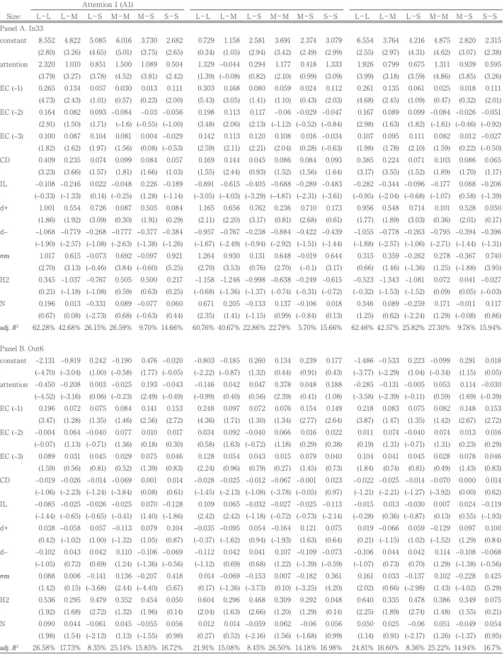
Table 7 reports the results for timeseries regressions of excess comovement on attention measurement and explanatory variables with lagged dependent variables based on Model 2 for sizesorted groups. Symbols “L,” “M,” and “S” express the largest, middle, and smallest cohorts of stocks, respectively, on the basis of their market values. Therefore, for example, “L‒L” means that large stocks constitute both cohorts.
Panel A reports the results for the combination of two stocks that belongs to the same sector in the 33 sector classifications (In33). The results as a whole resemble those in Table 6 Panel B, although with weaker impacts of the coefficients of the variable “attention” in the case “Attention 2.” Moreover, the adjusted coefficients of determination for combinations containing the smallest size are lower. Panel B presents the results for the remaining combinations of two stocks (Out6) not belonging to the In33 and In6 Out33. The results as a whole resemble those in Table 6 Panel D, although some unstable results appear similar to those in Panel A. Although the results as a whole do not offer a certain systematic feature, certain results represent slight instability. We think that this outcome requires further investigation, including the relationship with other investment styles.
C. Additional Tests for Effects of Investor Overconfidence on Excess Comovement
In this subsection, we examine the effects on ex cess comovement of both investor categorylearning behavior and overconfidence, as suggested by Peng and Xiong (2006), among stocks belonging to different sectors. In subsections 4.1 and 4.2, we reported that although excess comovement among stocks within the same sectors correlates strongly to attention gaps, excess comovement among stocks belonging to different sectors correlates to marketwide dispersions of analysts’ forecasts, not to relative information about
Table 7: Time-series regressions of excess comovement on attention measurement and explanatory variables with lagged ECs : Model 2 for size-sorted groups
Attention 1 (A1) Size: L-L L-M L-S M-M M-S S-S L-L L-M L-S M-M M-S S-S L-L L-M L-S M-M M-S S-S Panel A. In33 constant 8.552 4.822 5.085 6.016 3.730 2.682 0.729 1.158 2.581 3.691 2.374 3.079 6.554 3.764 4.216 4.875 2.820 2.315 (2.80) (3.26) (4.65) (5.01) (3.75) (2.65) (0.34) (1.05) (2.94) (3.42) (2.49) (2.99) (2.55) (2.97) (4.31) (4.62) (3.07) (2.38) attention 2.320 1.010 0.851 1.500 1.089 0.504 1.329 –0.044 0.294 1.177 0.418 1.333 1.926 0.799 0.675 1.311 0.939 0.595 (3.79) (3.27) (3.78) (4.52) (3.81) (2.42) (1.39) (–0.08) (0.82) (2.10) (0.99) (3.09) (3.99) (3.18) (3.59) (4.86) (3.85) (3.26) EC (–1) 0.265 0.134 0.057 0.030 0.013 0.111 0.303 0.168 0.080 0.059 0.024 0.112 0.261 0.135 0.061 0.025 0.018 0.111 (4.73) (2.43) (1.01) (0.57) (0.23) (2.00) (5.43) (3.05) (1.41) (1.10) (0.43) (2.03) (4.68) (2.45) (1.09) (0.47) (0.32) (2.01) EC (–2) 0.164 0.082 0.093 –0.084 –0.03 –0.056 0.198 0.113 0.117 –0.06 –0.029 –0.047 0.167 0.089 0.099 –0.084 –0.026 –0.051 (2.91) (1.50) (1.71) (–1.6) (–0.55) (–1.00) (3.48) (2.06) (2.13) (–1.12) (–0.52) (–0.84) (2.98) (1.63) (1.82) (–1.61) (–0.46) (–0.92) EC (–3) 0.100 0.087 0.104 0.081 0.004 –0.029 0.142 0.113 0.120 0.108 0.016 –0.034 0.107 0.095 0.111 0.082 0.012 –0.027 (1.82) (1.62) (1.97) (1.56) (0.08) (–0.53) (2.59) (2.11) (2.21) (2.04) (0.28) (–0.63) (1.98) (1.78) (2.10) (1.59) (0.22) (–0.50) CD 0.409 0.235 0.074 0.099 0.084 0.057 0.169 0.144 0.045 0.086 0.084 0.093 0.385 0.224 0.071 0.103 0.086 0.065 (3.23) (3.66) (1.57) (1.81) (1.66) (1.03) (1.55) (2.44) (0.93) (1.52) (1.56) (1.64) (3.17) (3.55) (1.52) (1.89) (1.70) (1.17) IL –0.108 –0.246 0.022 –0.048 0.226 –0.189 –0.891 –0.615 –0.405 –0.688 –0.289 –0.483 –0.282 –0.344 –0.096 –0.177 0.088 –0.206 (–0.33) (–1.33) (0.14) (–0.25) (1.28) (–1.14) (–3.05) (–4.03) (–3.29) (–4.87) (–2.31) (–3.61) (–0.95) (–2.04) (–0.68) (–1.07) (0.58) (–1.39) d+ 1.001 0.554 0.726 0.087 0.505 0.084 1.165 0.656 0.762 0.236 0.710 0.173 0.956 0.548 0.714 0.101 0.528 0.050 (1.86) (1.92) (3.09) (0.30) (1.91) (0.29) (2.11) (2.20) (3.17) (0.81) (2.68) (0.61) (1.77) (1.89) (3.03) (0.36) (2.01) (0.17) d– –1.068 –0.779 –0.268 –0.777 –0.377 –0.384 –0.957 –0.767 –0.238 –0.884 –0.422 –0.439 –1.055 –0.778 –0.263 –0.795 –0.394 –0.396 (–1.90) (–2.57) (–1.08) (–2.63) (–1.38) (–1.26) (–1.67) (–2.49) (–0.94) (–2.92) (–1.51) (–1.44) (–1.88) (–2.57) (–1.06) (–2.71) (–1.44) (–1.31) σm 1.017 0.615 –0.073 0.692 –0.097 0.921 1.264 0.930 0.131 0.648 –0.019 0.644 0.315 0.359 –0.262 0.278 –0.367 0.740 (2.70) (3.13) (–0.46) (3.84) (–0.60) (5.25) (2.70) (3.53) (0.76) (2.70) (–0.1) (3.17) (0.66) (1.46) (–1.36) (1.25) (–1.88) (3.95) H2 0.345 –1.037 –0.767 0.505 0.500 0.217 –1.158 –1.246 –0.998 –0.638 –0.249 –0.615 –0.523 –1.343 –1.081 0.072 0.041 –0.027 (0.21) (–1.18) (–1.08) (0.59) (0.63) (0.25) (–0.68) (–1.36) (–1.37) (–0.74) (–0.31) (–0.72) (–0.32) (–1.53) (–1.52) (0.09) (0.05) (–0.03) N 0.196 0.013 –0.331 0.089 –0.077 0.060 0.671 0.205 –0.133 0.137 –0.106 0.018 0.346 0.089 –0.259 0.171 –0.011 0.117 (0.67) (0.08) (–2.73) (0.68) (–0.63) (0.44) (2.35) (1.41) (–1.15) (0.99) (–0.84) (0.13) (1.25) (0.62) (–2.24) (1.29) (–0.08) (0.86) adj. R2 62.28% 42.68% 26.15% 26.59% 9.70% 14.66% 60.76% 40.67% 22.86% 22.79% 5.70% 15.66% 62.46% 42.57% 25.82% 27.30% 9.78% 15.94% Panel B. Out6 constant –2.131 –0.819 0.242 –0.190 0.476 –0.020 –0.803 –0.185 0.260 0.134 0.239 0.177 –1.486 –0.533 0.223 –0.099 0.291 0.018 (–4.70) (–3.04) (1.00) (–0.58) (1.77) (–0.05) (–2.22) (–0.87) (1.32) (0.44) (0.91) (0.43) (–3.77) (–2.29) (1.04) (–0.34) (1.15) (0.05) attention –0.450 –0.208 0.003 –0.025 0.193 –0.043 –0.146 0.042 0.047 0.378 0.048 0.188 –0.285 –0.131 –0.005 0.053 0.114 –0.030 (–4.52) (–3.16) (0.06) (–0.23) (2.49) (–0.49) (–0.99) (0.40) (0.56) (2.39) (0.41) (1.08) (–3.58) (–2.39) (–0.11) (0.59) (1.69) (–0.39) EC (–1) 0.196 0.072 0.075 0.084 0.141 0.153 0.248 0.097 0.072 0.076 0.154 0.149 0.218 0.083 0.075 0.082 0.148 0.153 (3.47) (1.28) (1.35) (1.46) (2.56) (2.72) (4.36) (1.71) (1.30) (1.34) (2.77) (2.64) (3.87) (1.47) (1.35) (1.42) (2.67) (2.72) EC (–2) –0.004 0.064 –0.040 0.077 0.010 0.017 0.034 0.092 –0.040 0.066 0.016 0.022 0.011 0.074 –0.040 0.074 0.013 0.016 (–0.07) (1.13) (–0.71) (1.36) (0.18) (0.30) (0.58) (1.63) (–0.72) (1.18) (0.29) (0.38) (0.19) (1.31) (–0.71) (1.31) (0.23) (0.29) EC (–3) 0.089 0.031 0.045 0.029 0.075 0.046 0.128 0.054 0.043 0.015 0.079 0.040 0.104 0.041 0.045 0.028 0.078 0.046 (1.59) (0.56) (0.81) (0.52) (1.39) (0.83) (2.24) (0.96) (0.79) (0.27) (1.45) (0.73) (1.84) (0.74) (0.81) (0.49) (1.43) (0.83) CD –0.019 –0.026 –0.014 –0.069 0.001 0.014 –0.028 –0.025 –0.012 –0.067 –0.001 0.023 –0.022 –0.025 –0.014 –0.070 0.000 0.014 (–1.06) (–2.23) (–1.24) (–3.84) (0.08) (0.61) (–1.45) (–2.13) (–1.08) (–3.78) (–0.05) (0.97) (–1.21) (–2.21) (–1.27) (–3.92) (0.00) (0.62) IL –0.085 –0.025 –0.026 –0.025 0.070 –0.128 0.109 0.065 –0.032 –0.027 –0.025 –0.113 –0.015 0.013 –0.030 0.007 0.024 –0.119 (–1.44) (–0.65) (–0.65) (–0.41) (1.40) (–1.86) (2.42) (2.42) (–1.18) (–0.72) (–0.73) (–2.14) (–0.28) (0.36) (–0.87) (0.13) (0.55) (–1.93) d+ 0.038 –0.058 0.057 –0.113 0.079 0.104 –0.035 –0.095 0.054 –0.164 0.121 0.075 0.019 –0.066 0.059 –0.129 0.097 0.100 (0.42) (–1.02) (1.00) (–1.32) (1.05) (0.87) (–0.37) (–1.62) (0.94) (–1.93) (1.63) (0.64) (0.21) (–1.15) (1.02) (–1.52) (1.29) (0.84) d– –0.102 0.043 0.042 0.110 –0.106 –0.069 –0.112 0.042 0.041 0.107 –0.109 –0.073 –0.106 0.044 0.042 0.114 –0.108 –0.068 (–1.05) (0.72) (0.69) (1.24) (–1.36) (–0.56) (–1.12) (0.69) (0.68) (1.22) (–1.39) (–0.59) (–1.07) (0.73) (0.70) (1.29) (–1.38) (–0.56) σm 0.088 0.006 –0.141 0.136 –0.207 0.418 0.014 –0.069 –0.153 0.007 –0.182 0.361 0.161 0.033 –0.137 0.102 –0.228 0.425 (1.42) (0.15) (–3.68) (2.44) (–4.40) (5.67) (0.17) (–1.36) (–3.73) (0.10) (–3.25) (4.20) (2.02) (0.66) (–2.98) (1.43) (–4.02) (5.29) H2 0.536 0.295 0.479 0.352 0.454 0.050 0.604 0.296 0.468 0.309 0.292 0.048 0.640 0.335 0.478 0.386 0.349 0.075 (1.92) (1.68) (2.72) (1.32) (1.96) (0.14) (2.04) (1.63) (2.66) (1.20) (1.29) (0.14) (2.25) (1.89) (2.74) (1.48) (1.55) (0.21) N 0.090 0.044 –0.061 0.045 –0.055 0.056 0.012 0.014 –0.059 0.062 –0.06 0.056 0.050 0.025 –0.06 0.051 –0.049 0.054 (1.98) (1.54) (–2.12) (1.13) (–1.55) (0.98) (0.27) (0.52) (–2.16) (1.56) (–1.68) (0.99) (1.14) (0.91) (–2.17) (1.26) (–1.37) (0.95) adj. R2 26.58% 17.73% 8.35% 25.14% 15.85% 16.72% 21.91% 15.08% 8.45% 26.50% 14.18% 16.98% 24.81% 16.60% 8.36% 25.22% 14.94% 16.7% Note: Symbols “L,” “M,” and “S” express the largest, middle, and smallest cohorts of stocks on the basis of their market values, respectively. Therefore,
for example, “L‒L” means that both cohorts are constituted by large stocks. The symbols for the explanatory variables are the same as in Table 4. “EC” is excess comovement and the number in parentheses is a lag of a month’s interval. tstatistics are reported in parentheses. “adj. R2” denotes
individual paired stocks. To investigate the latter finding further, we evaluate the combined effect of the forecast dispersions and investor overconfidence. We expect that, during periods when analysts’ forecasts disperse, because investors cannot process the firm specific information correctly, they process market information more preferentially by categorylearning and, consequently, their overconfidence causes excess comovement. The empirical evidence in Peng, Xiong, and Bollerslev (2007) is consistent with the hypothesis that when marketwide uncertainty increases, investors shift their attention to processing market information. We use the magnitude of foreign investors’ buying and selling pressure as a proxy variable for investor overconfidence. This magnitude is measured as absolute values of monthly net trading values that subtract “sales” from “purchases” for TSE First Section stock transactions by foreign investors. In other words, we think that large net buying and net selling express
investor overconfidence. Iihara, Kato, and Tokunaga (2001) find that foreign investor herding affects stock prices, using twenty years of ownership data in the Japanese stock market. They conclude that foreign investors’ trades are related to information.
Table 8 reports the results for timeseries regressions that incorporate the influence of foreign investors’ behavior on the coefficients of the information heterogeneity variable (H2) in Model M2 in Table 6. Model 2’ adds the absolute values of monthly net trading values (|F|) as a proxy variable for investor overconfidence to Model 2 of Table 6. The estimation results reveal that this additional variable does not have significantly linear relationships with excess comovement in any case, regardless of the sector. Model 2” allows the coefficients of information hetero geneity to vary with the level of investor overconfidence. The estimation results reveal that the coefficients of the combined effect for the crosssector (“Out6”) correlate
Table 8: Time-series regressions incorporating the influence of foreign investors’ behavior into information heterogeneity in Model 2
Group: In33 Out6
Attention: A1 A2 A3 A1 A2 A3 A1 Model: M2’ M2” M2’ M2” M2’ M2” M2’ M2” M2’ M2” M2’ M2” constant 5.027 4.997 1.655 1.709 3.820 3.830 –0.204 –0.213 –0.053 –0.062 –0.149 –0.158 (4.71) (4.77) (1.93) (2.01) (4.23) (4.3) (–1.31) (–1.4) (–0.40) (–0.47) (–1.09) (–1.18) attention 1.516 1.513 0.944 0.937 1.331 1.336 –0.043 –0.047 0.069 0.061 –0.025 –0.029 (5.46) (5.47) (2.15) (2.13) (5.78) (5.79) (–1.02) (–1.11) (1.05) (0.92) (–0.69) (–0.81) EC (–1) 0.138 0.139 0.194 0.193 0.137 0.136 0.235 0.229 0.236 0.231 0.235 0.229 (2.57) (2.57) (3.54) (3.53) (2.56) (2.55) (4.12) (4.02) (4.14) (4.06) (4.13) (4.03) EC (–2) –0.014 –0.013 0.021 0.020 –0.011 –0.01 0.117 0.110 0.116 0.110 0.117 0.111 (–0.26) (–0.24) (0.38) (0.36) (–0.21) (–0.19) (2.00) (1.89) (1.98) (1.89) (2.01) (1.90) EC (–3) 0.058 0.058 0.105 0.106 0.069 0.069 0.017 0.017 0.010 0.010 0.019 0.019 (1.13) (1.12) (1.98) (2.01) (1.36) (1.35) (0.30) (0.29) (0.17) (0.17) (0.32) (0.32) CD 0.150 0.150 0.118 0.117 0.150 0.150 –0.02 –0.019 –0.019 –0.018 –0.02 –0.019 (3.41) (3.42) (2.59) (2.56) (3.45) (3.44) (–2.66) (–2.65) (–2.47) (–2.47) (–2.66) (–2.64) IL 0.057 0.056 –0.546 –0.548 –0.081 –0.083 –0.008 –0.006 0.008 0.011 0.002 0.003 (0.38) (0.37) (–4.50) (–4.47) (–0.61) (–0.62) (–0.30) (–0.25) (0.47) (0.67) (0.09) (0.16) d+ 0.419 0.417 0.522 0.535 0.415 0.421 0.013 0.007 0.000 –0.006 0.011 0.004 (1.83) (1.83) (2.19) (2.26) (1.83) (1.86) (0.34) (0.17) (–0.01) (–0.15) (0.28) (0.11) d– –0.649 –0.65 –0.705 –0.704 –0.658 –0.66 0.005 0.007 0.005 0.007 0.005 0.007 (–2.88) (–2.89) (–3.01) (–3.01) (–2.94) (–2.95) (0.13) (0.18) (0.13) (0.18) (0.14) (0.19) σm 0.471 0.471 0.490 0.497 0.037 0.038 –0.018 –0.02 –0.049 –0.05 –0.013 –0.014 (3.27) (3.26) (2.60) (2.65) (0.20) (0.21) (–0.75) (–0.86) (–1.62) (–1.65) (–0.43) (–0.47) H2 0.165 0.263 –0.895 –1.061 –0.362 –0.27 0.305 0.212 0.315 0.239 0.320 0.231 (0.25) (0.37) (–1.33) (–1.48) (–0.57) (–0.39) (2.61) (1.71) (2.73) (1.99) (2.77) (1.91) |F| –0.07 0.138 –0.044 0.048 0.040 0.045 (–0.36) (0.70) (–0.23) (1.48) (1.24) (1.41) H2* |F| –0.212 0.349 –0.201 0.217 0.186 0.211 (–0.34) (0.54) (–0.32) (2.07) (1.79) (2.01) N 0.096 0.094 0.234 0.235 0.186 0.182 0.006 0.010 0.005 0.008 0.004 0.007 (0.92) (0.89) (2.15) (2.14) (1.81) (1.76) (0.38) (0.59) (0.32) (0.48) (0.22) (0.42) adj. R2 45.45% 45.44% 40.99% 40.95% 46.02% 46.02% 27.69% 28.19% 27.71% 28.09% 27.56% 28.05%
Note: The symbols for the explanatory variables are the same as in Table 4. “EC” is excess comovement, and the number in parentheses is a lag of a month’s interval. “|F|” denotes the absolute values of monthly net trading values by foreign investors. tstatistics are reported in parentheses. “adj.