The 50th Anniversary of Gr¨obner Bases pp. 253–352
Algorithms for D-modules, integration, and
generalized functions with applications to statistics
Toshinori Oaku
Abstract.
This is an enlarged and revised version of the slides presented in a series of survey lectures given by the present author at MSJ SI 2015 in Osaka. The goal is to introduce an algorithm for computing a holo-nomic system of linear (ordinary or partial) differential equations for the integral of a holonomic function over the domain defined by polyno-mial inequalities. It applies to the cumulative function of a polynopolyno-mial of several independent random variables with e.g., a normal distribution or a gamma distribution. Our method consists in Gr¨obner basis com-putation in the Weyl algebra, i.e., the ring of differential operators with polynomial coefficients. In the algorithm, generalized functions are in-evitably involved even if the integrand is a usual function. Hence we need to make sure to what extent purely algebraic method of Gr¨obner basis applies to generalized functions which are based on real analysis.
Contents
1. Introduction: aim and an example from statistics 254
2. Basics of D-module theory 258
3. Gr¨obner bases in the ring of differential operators 275 4. Distributions as generalized functions 291 5. D-module theoretic integration algorithm 307 6. Integration of holonomic distributions 322
Received August 30, 2016.
2010 Mathematics Subject Classification. 13N10, 13P10, 46F10, 62E15. Key words and phrases. D-module, Gr¨obner basis, generalized function, probability density function.
§1. Introduction: aim and an example from statistics
A univariate function is called holonomic if it satisfies a (non-trivial) linear ordinary differential equation. Special functions such as the hy-pergeometric function or the Bessel function are holonomic, as well as ra-tional functions and their exponential and logarithm. As is well-known, the solutions of a linear ordinary differential equation constitute a finite dimensional vector space.
A D-module is a system of linear (partial or ordinary) differential equations with polynomial (or analytic function) coefficients. There is a special class of D-modules which are called holonomic, the solution spaces of which are finite dimensional vector spaces. This notion was introduced by Mikio Sato and J. Bernstein independently. Bernstein [2], [3] introduced a special class of linear partial differential equations with polynomial coefficients which was called the Bernstein class in [4]. On the other hand, Sato and his collaborators M. Kashiwara, T. Kawai [31] introduced the notion of a holonomic system, which was called at first a maximally overdetermined system, in the category of differential operators with analytic coefficients.
A holonomic function is a differentiable or a generalized function which is a solution of a holonomic system. For example, exp(f ) = ef is
a holonomic function for any polynomial f = f (x1, . . . , xn). In
statis-tics, most of important probability density functions, such as those of the multivariate normal distribution and the gamma distribution are holo-nomic. Our aim is to find a holonomic system which is satisfied by the integral of a holonomic function over the domain defined by polynomial inequalities.
As an example, let us consider the integral F (t) = 1 2π ! D(t) exp"−12(x2+ y2)#dxdy, D(t) ={(x, y) ∈ R2 | xy ≤ t}. It can be regarded as the cumulative distribution function of xy with (x, y) being a random vector with the two dimensional standard normal (Gaussian) distribution. Let us introduce the Heaviside function Y (t) such that Y (t) = 1 for t > 0 and Y (t) = 0 for t < 0. (One does not need to mind the value at t = 0.) Y (t) is discontinuous at t = 0 and its derivative Y′(t) as a generalized function coincides with Dirac’s delta
function δ(t). As a generalized function, δ(t) vanishes outside of t = 0 and tδ(t) = 0 holds everywhere inR.
By using the Heaviside function, we rewrite F (t) as F (t) = 1
2π !
R2
Differentiation under the integral sign yields v(t) := F′(t) = 1 2π ! R2 exp"−1 2(x 2+ y2)#δ(t − xy) dxdy. The integrand u(x, y, t) := exp"−12(x2+ y2)#δ(t− xy) satisfies a
holo-nomic system
(∂y+ x∂t+ y)u = (∂x+ y∂t+ x)u = (t− xy)u = 0
with ∂x = ∂/∂x, ∂y = ∂/∂y, ∂t = ∂/∂t as is easily checked. The
integration algorithm for D-modules (see 5.2) outputs an answer (1) (t∂2t+ ∂t− t)v(t) = 0.
In fact, we have an equality
y∂t(∂y+ x∂t+ y)− y(∂x+ y∂t+ x) + (∂2t− 1)(t − xy)
=−∂xy + ∂yy∂t+ t∂t2+ ∂t− t
in the ring of differential operators. Since the differential operator on the left-hand side annihilates u(x, y, t), we get
(t∂2 t + ∂t− t)v(t) = 1 2π ! R2 (t∂2 t + ∂t− t)u(x, y, t) dxdy = 1 2π ! R2 ∂x(yu(x, y, t)) dxdy− 1 2π ! R2
∂y(y∂tu(x, y, t)) dxdy = 0.
The integrals on the last line vanish since yu(x, y, t) and y∂tu(x, y, t) are
‘rapidly decreasing’ in x, y; this reasoning shall be made precise in 4.3. It follows that w(z) := v(−iz) satisfies the Bessel differential equa-tion z2d 2w dz2 + z dw dz + z 2w = 0.
Together with the property that v(t)→ 0 as t → ±∞ and v(−t) = v(t), this implies
v(t) = CH0(1)(i|t|) (t̸= 0)
with some constant C, where H0(1)(z) is a Hankel function. This fact was
observed, for example, by Wishart and Bartlett [36] as a special case. Note that v(t) is discontinuous at t = 0 but is integrable and satisfies (1) in the sense of generalized functions on the whole real line R.
It also follows from (1) that the characteristic function, i.e., the Fourier transform ˆ v(τ ) = ! ∞ −∞ eitτv(t) dt = ! R2 exp"iτ xy−1 2(x 2+ y2)#dxdy
satisfies a differential equation (τ2+ 1) d
dτv(τ ) + τ ˆˆ v(τ ) = 0.
Together with ˆv(0) = 1, this implies ˆv(τ ) = (τ2+ 1)−1/2. Thus we get
an alternative expression
v(t) = V+(t + i0) + V−(t− i0) = limε
→+0(V+(t + iε) + V−(t− iε))
as a hyperfunction of Mikio Sato ([30]) with V+(t + is) = 1
2π ! 0
−∞
exp(−i(t + is)τ) √
τ2+ 1 dτ,
V−(t + is) = 2π1
! ∞ 0
exp(−i(t + is)τ) √
τ2+ 1 dτ,
where V+(t+is) and V−(t+is) are holomorphic functions of t+is on the
upper half plane s > 0 and on the lower half plane s < 0 respectively. In general, for a holonomic function u(x, y) with x = (x1, . . . , xn)
and y = (y1, . . . , yd), let us consider the integral
v(y) = !
D(y)
u(x, y) dx1· · · dxn,
D(y) ={x ∈ Rn| fj(x, y)≥ 0 (1 ≤ j ≤ m)}
with real polynomials f1, . . . , fmin (x, y). We rewrite it as
v(y) = !
Rn
u(x, y)Y (f1(x, y))· · · Y (fm(x, y)) dx1· · · dxn
and apply the D-module theoretic integration algorithm to obtain a holonomic system for v(y), assuming that the integrand and its deriva-tives are ‘rapidly decreasing’ with respect to the integration variables x. In the process, we also need an algorithm to compute a holonomic sys-tem for the product uY (f1)· · · Y (fm) as a generalized function. Then
the D-module theory assures us that the obtained system of differential equations for v(y) is holonomic.
Finally, let us remark that we cannot use differential operators with rational function coefficients since generalized functions are involved in the computation. For example, x∂xY (x) = 0 does not imply ∂xY (x) =
δ(x) = 0; we cannot factor out x.
The organization of this article is as follows:
Section 2 is a hopefully concise exposition on the very beginning of the D-module theory; the central subject is holonomic D-modules. More advanced topics such as D-modules with regular singularities are not treated. The presentation is almost self-contained with some arguments and examples supplied in the next section after armed with Gr¨obner bases.
In Section 3, we introduce Gr¨obner bases over the ring of differential operators. One point is that we can compute Gr¨obner bases with respect to arbitrary monomial orders that are not necessarily well-orders, which will be needed in the integration algorithm. We also describe first ap-plications of Gr¨obner bases to D-module theory: computation of the characteristic variety, and a proof of the equivalence of the two defini-tions of holonomicity introduced in the previous section.
In Section 4, we briefly review the theory of distributions in the sense of generalized functions from our viewpoint, with mention of the relation with statistical distributions. Especially, we introduce some classes of distributions which are adapted to our integration algorithm developed in the following sections.
Section 5 is a review on the integration of D-modules both from theoretical and algorithmic viewpoints; the material should be more or less standard by now.
In the first subsection of Section 6, we give some examples of inte-grals which correspond to random variables with respect to the multi-variate standard normal distribution such as the example above. In a somewhat technical subsection 6.2, we introduce an algorithm to com-pute a holonomic system for the product of complex powers of polyno-mials and a holonomic function. This enables us to compute, in 6.3, a holonomic system for the integral of a holonomic function over the domain defined by arbitrary polynomial inequalities. Finally in 6.4, we treat the integral of a function with some auxiliary parameters which satisfies a holonomic difference-differential system.
The author would like to express his deepest gratitude to the orga-nizers of MSJ SI 2015, especially to Takayuki Hibi, for the invitation and the encouragement. At the same time, the author is grateful to Akimichi Takemura and Nobuki Takayama also for drawing his attention to statis-tics; their influence is reflected in the appended last phrase of the title.
This work was supported by JSPS Grant-in-Aid for Scientific Research (C) 26400123.
§2. Basics of D-module theory
We review the theory of D-modules, more precisely, of modules over the Weyl algebra, which was initiated by J. Bernstein [2], [3]. A stan-dard reference is the first chapter of [4]. A D-module corresponds to a system of linear (ordinary or partial) differential equations with poly-nomial coefficients. The notion of holonomic modules, also called the Bernstein class of modules, and its characterizations are most essential. We remark that the notion of holonomic modules over the ring of dif-ferential operators with complex analytic coefficients was independently introduced by M. Sato, T. Kawai, and M. Kashiwara [31].
2.1. The ring of differential operators
Let K be an arbitrary field of characteristic zero. We denote by K[x] := K[x1, . . . , xn] the ring of polynomials in indeterminates
x = (x1, . . . , xn) with coefficients inK. A derivation θ : K[x] → K[x] is
aK-linear map that satisfies
θ(f g) = θ(f )g + f θ(g) (∀f, g ∈ K[x]).
The set DerKK[x] of the derivations constitutes a K[x]-module. For i = 1, . . . , n, define a derivation ∂i = ∂xi by the partial derivative
∂i : K[x] ∋ f +−→
∂f
∂xi ∈ K[x].
Then ∂1, . . . , ∂n are aK[x]-basis of DerKK[x]. In fact, if θ ∈ DerKK[x],
then it is easy to see that
θ = θ(x1)∂1+· · · + θ(xn)∂n.
Let EndKK[x] be the K-algebra consisting of the K-linear endo-morphisms ofK[x]. The ring Dn is defined to be the K-subalgebra of
EndKK[x] that is generated by K[x] and DerKK[x], or equivalently, by x1, . . . , xn and ∂1, . . . , ∂n. This ring Dn is called the ring of differential
operators in the variables x = (x1, . . . , xn) with polynomial coefficients,
or, more simply, the n-th Weyl algebra overK.
An element a = a(x) ofK[x] is regarded as an element of Dn as the
multiplication operator f +→ af for f ∈ K[x]. With this identification, Dn containsK[x] as a subring. The ring Dn is a non-commutative
in Dn satisfies
∂ia = a∂i+ ∂i(a) = a∂i+ ∂a
∂xi
(i = 1, . . . , n).
For a multi-index α = (α1, . . . , αn) ∈ Nn with N = {0, 1, 2, . . . },
we use the notation xα = xα1
1 · · · xαnn, ∂α = ∂xα = ∂1α1· · · ∂αnn, and
|α| = α1+· · · + αn. Then an element P of Dn is uniquely written in a
finite sum P = P (x, ∂) = $ α,β∈Nn aα,βxα∂β= $ β∈Nn aβ(x)∂β
with aα,β∈ K and aβ(x) =%αaα,βxα, which is called the normal form
of P . In fact, aβ(x) are uniquely determined by the action of P onK[x]
as follows: First we have a(0,...,0)(x) = P 1. Next, we have
a(1,0,...,0)(x) = P x1− a(0,...,0)(x)x1,
and so on. Here we need the assumption that the characteristic of K is zero.
Introducing commutative indeterminates ξ = (ξ1, . . . , ξn) which
cor-responds to ∂, we associate with this P a polynomial P (x, ξ) := $
α,β∈Nn
aα,βxαξβ ∈ K[x, ξ] = K[x1, . . . , xn, ξ1, . . . , ξn]
and call it the total symbol of P . Note that P must be in the normal form when ξ is substituted for ∂. By this correspondence, Dn is isomorphic
to K[x, ξ] as a K-vector space but not as a ring.
The product R = P Q in Dn can be effectively computed by using
the Leibniz formula
(2) R(x, ξ) = $ ν∈Nn 1 ν! & ∂ ∂ξ 'ν P (x, ξ)· & ∂ ∂x 'ν Q(x, ξ)
in terms of total symbols, where we use the notation ν! = ν1!· · · νn! for
ν = (ν1, . . . , νn)∈ Nn.
Example 2.1. Set n = 1 and write x = x1 and ∂ = ∂1. Consider
the product R := ∂mxm with a non-negative integer m. Since the total symbols of ∂mand xm are ξmand xmrespectively, the Leibniz formula
(2) gives the total symbol R(x, ξ) as R(x, ξ) = ∞ $ ν=0 1 ν! & ∂ ∂ξ 'ν ξm · & ∂ ∂x 'ν xm = m $ ν=0 1 ν!{m(m − 1) · · · (m − ν + 1)} 2 ξm−νxm−ν. This implies ∂mxm= m $ ν=0 1 ν!{m(m − 1) · · · (m − ν + 1)} 2 xm−ν∂m−ν. Exercise 1. Show that an element P =%β∈Naβ(x)∂β of Dn with
aβ(x) ∈ K[x] defines the zero endomorphism of K[x] if and only if
aβ(x) = 0 for any β.
Exercise 2. Prove the Leibniz formula (2).
Exercise 3. Set n = 1 and x = x1, ∂ = ∂1. For a positive integer
m, prove the formulae
xm∂m= x∂(x∂−1) · · · (x∂−m+1), ∂mxm= ∂x(∂x+1)· · · (∂x+m−1). 2.2. The D-module formalism
Given P1, . . . , Pr∈ Dn, let us consider a system of linear (partial or
ordinary) differential equations
(3) P1u =· · · = Pru = 0
for an unknown function u. Let I := DnP1+· · · + DnPrbe the left ideal
of Dn generated by P1, . . . , Pr. Then (3) is equivalent to
P u = 0 (∀P ∈ I).
Here we suppose that the unknown function u belongs to some ‘function space’F which is a left Dn-module.
For F to be a left Dn-module, it is necessary that any function
f belonging to F be infinitely differentiable and multiplication ah by an arbitrary polynomial a ∈ K[x] make sense. Here are examples of ‘function spaces’:
Example 2.2. By the definition, K[x] has a natural structure of left Dn-module since Dn is a subalgebra of EndKK[x]. So K[x] has two
structures: a subring of Dn and a left Dn-module. Hence for f ∈ K[x]
• P f as the product in Dn with f regarded as an element of the
subring K[x] of Dn.
• P f as the action of P on the element f of the left Dn-module
K[x]. In other words, we regard f as a function subject to derivations.
This might cause some confusion. In [29], the action of P on an element f of a left Dn-module is conspicuously denoted P • f for distinction.
We shall denote, if needed, P f = P (f ) to clarify the action of P on f , and P f = P· f to emphasize that it is the product in Dn, following the
traditional notation in D-module theory.
Example 2.3. The fieldK(x) = K(x1, . . . , xn) of rational functions
has a natural structure of left Dn-module. For a point a = (a1, . . . , an)
of the affine space Kn, the setK[x]
a of regular functions at a, i.e., the
elements ofK(x) whose denominators do not vanish at a, also has a nat-ural structure of Dn-module. More generally, the localizationK[x][S−1]
by a multiplicative subset S of K[x] is also a left Dn-module.
Example 2.4. Set K = C. Let C∞(U ) be the set of the
complex-valued C∞functions on an open set U of the n-dimensional real
Euclid-ean spaceRn. Then each ∂
i acts on C∞(U ) as differentiation and xi as
multiplication. This makes C∞(U ) a left D
n-module. Let C0∞(U ) be
the set of C∞ functions on U with compact support. More precisely, f ∈ C∞(U ) belongs to C∞
0 (U ) if and only if there is a compact subset
K of U such that f (x) = 0 for any x ∈ U \ K. Then C∞
0 (U ) is a left
Dn-submodule of C∞(U ).
Other examples of suchF with K = C are the set O(Ω) of holomor-phic functions on an open subset Ω ofCn, the setD′(U ) of the Schwartz
distributions on an open subset U ofRn, and the set S′(Rn) of tempered
distributions, which shall be introduced later, as well as the setB(U) of the hyperfunctions (of Mikio Sato) on an open subset U of Rn.
Now for a left ideal I of Dn, consider the residue module
M := Dn/I, which is a left Dn-module generated by the residue class 1
of 1 ∈ K[x] ⊂ Dn. Fix a left Dn-module F as your favorite function
space. A map ϕ : M → F is Dn-linear, or a Dn-homomorphism, if
ϕ(u + v) = ϕ(u) + ϕ(v), ϕ(P u) = P ϕ(u) (∀u, v ∈ M, ∀P ∈ Dn).
Let HomDn(M,F) be the set of the Dn-homomorphisms of M to F,
which is aK-vector space. Since M is generated by 1 as left Dn-module,
ϕ∈ HomDn(M,F) is uniquely determined by ϕ(1) ∈ F. On the other
annihilated by I, i.e., P ϕ(1) = 0 for any P ∈ I. In conclusion, we have aK-isomorphism
HomDn(M,F) ∋ ϕ
∼
+−→ ϕ(1) ∈ {f ∈ F | P f = 0 (∀P ∈ I)}. For an element u of a left Dn-moduleF, we define the annihilator
of u in Dn to be the left ideal
AnnDnu ={P ∈ Dn| P u = 0}.
Then we have
I = AnnDn1 ={P ∈ Dn| P 1 = 0 ∈ M}
by the definition.
We started with a left ideal I of Dngenerated by given P1, . . . , Pr∈
Dn and considered a left Dn-module M = Dn/I. We can argue in the
reverse order: Let M be a finitely generated left Dn-module and let
u1, . . . , um ∈ M be generators of M, i.e., assume that for any u ∈ M,
there exist P1, . . . , Pm∈ Dn such that u = P1u1+· · · + Pmum. Set
N :={(P1, . . . , Pm)∈ (Dn)m| P1u1+· · · + Pmum= 0},
which is a left Dn-submodule of the free module (Dn)m.
Since Dn is a left (and right) Noetherian ring (this can be proved
by using a Gr¨obner basis in Dn), N is also finitely generated over Dn.
Hence there exist
Qi= (Qi1, . . . , Qim)∈ (Dn)m (i = 1, . . . , r)
which generate N as left Dn-module. Then we have an exact sequence
of left Dn-modules (4) (Dn)r ψ −→ (Dn)m ϕ −→ M −→ 0,
which is called a presentation of M . Here ϕ and ψ are homomorphisms of left Dn-modules defined by, for Pi∈ Dn,
ϕ((P1, . . . , Pm)) = P1u1+· · · + Pmum, ψ((P1, . . . , Pr)) =(P1 · · · Pr) ⎛ ⎜ ⎝ Q11 · · · Q1m .. . ... Qr1 · · · Qrm ⎞ ⎟ ⎠ and N = ker ϕ = im ψ holds.
From (4) we get an exact sequence 0−→ HomDn(M,F) ϕ∗ −→ HomDn((Dn) m, F)−→ Homψ∗ Dn((Dn) r, F). Since HomDn((Dn) m,
F) is isomorphic to Fm, this yields
0−→ HomDn(M,F)
ϕ∗
−→ Fm ψ−→ F∗ r.
Regarding the elements of Fm as column vectors, we have, for
h∈ HomDn(M,F) and f1, . . . , fm∈ F, ϕ∗(h) = ⎛ ⎜ ⎝ h(u1) .. . h(um) ⎞ ⎟ ⎠ , ψ∗ ⎛ ⎜ ⎝ ⎛ ⎜ ⎝ f1 .. . fm ⎞ ⎟ ⎠ ⎞ ⎟ ⎠ = ⎛ ⎜ ⎝ Q11 · · · Q1m .. . ... Qr1 · · · Qrm ⎞ ⎟ ⎠ ⎛ ⎜ ⎝ f1 .. . fm ⎞ ⎟ ⎠ . Hence we have an isomorphism
HomDn(M,F) ∼= Ker ψ∗=0t(f 1, . . . , fm)∈ Fm| m $ j=1 Qijfj = 0 (i = 1, . . . , r) 1
asK-vector space. Note that the generators u1, . . . , umof M also satisfy
the same equations
m
$
j=1
Qijuj= 0 (i = 1, . . . , r)
in M . In this way, we can regard a finitely generated left Dn-module M
as a system of linear differential equations for unknown functions in a function space which correspond to generators of M .
Example 2.5. Let us considerK[x] as a left Dn-module. Since Dn
containsK[x] as a subring, K[x] is generated by 1 as a left Dn-module.
For P ∈ Dn, there exist Q1, . . . , Qn∈ Dn and r(x)∈ K[x] such that
P = Q1∂1+· · · + Qn∂n+ r(x).
Then the action of P on 1 is P (1) = r(x), which vanishes if and only if r(x) = 0. This impliesK[x] ∼= Dn/(Dn∂1+· · · + Dn∂n) and a
presenta-tion ofK[x] is given by (Dn)n · t(∂ 1,...,∂n) −→ Dn ϕ −→ K[x] −→ 0
with ϕ(P ) = P (1). In the same way we can show
HomDn(K[x], F) ∼= {f ∈ F | ∂1f =· · · = ∂nf = 0} = K
forF = K[x], K(x), K[x]a, or for F = C∞(U ) with an open connected
set U ofRn ifK = C.
Exercise 4. Confirm the formulae above for ϕ∗ and ψ∗.
Exercise 5. Construct a C-isomorphism HomDn(C[x], C∞(U )) ∼=
C for an open connected set U of Rn, where D
nis the n-th Weyl algebra
overC. What happens if U is not connected? 2.3. Weight vector and filtration A weight vector w for Dn is an integer vector
w = (w1, . . . , wn; wn+1,· · · , w2n)∈ Z2n
with the conditions wi+ wn+i≥ 0 for i = 1, . . . , n, which are necessary
in view of the commutation relation ∂ixi= xi∂i+1 in Dn. For a nonzero
differential operator P of the form P =%α,β∈Nnaα,βxα∂β, we define its
w-order to be
ordw(P ) = max{⟨w, (α, β)⟩ | aα,β ̸= 0}
with
⟨w, (α, β)⟩ := w1α1+· · · + wnαn+ wn+1β1+· · · + w2nβn.
We set ordw(0) :=−∞. A weight vector w induces the w-filtration
Fkw(Dn) :={P ∈ Dn | ordw(P )≤ k} (k∈ Z)
on the ring Dn. In general, for twoK-subspaces V, W of Dn, we denote
by V W theK-subspace of Dnspanned by products P Q with P ∈ V and
Q∈ W .
The w-filtration satisfies the properties: Fw k (Dn)⊂ Fk+1w (Dn), 2 k∈Z Fw k (Dn) = Dn, 1∈ Fw 0(Dn), Fkw(Dn)Flw(Dn)⊂ Fk+lw (Dn), 3 k∈Z Fw k (Dn) ={0}.
The w-graded ring associated with this filtration is defined to be grw(Dn) :=
4
k∈Z
Let P be a nonzero element of Dn with m := ordw(P ). Then we
denote by σw(P ) the residue class of P in grw
k(Dn)⊂ grw(Dn). We set
σw(0) = 0. It is easy to see that σw(P Q) = σw(P )σw(Q) holds for any
P, Q∈ Dn by using the Leibniz formula.
If wi+ wn+i> 0, then the w-order of ∂ixi− xi∂i= 1 is zero while
that of xi∂iis positive. Hence σw(xi) and σw(∂i) commute in grw(Dn).
In this case, we denote σw(x
i) and σw(∂i) simply by xi and ξiregarding
these as commutative indeterminates.
On the other hand, if wi+ wn+i= 0, then we have
σw(∂i)σw(xi)− σw(xi)σw(∂i) = 1
in grw(D
n), the same commutation relation as that for xi and ∂i in Dn.
Hence we will denote σw(x
i) and σw(∂i) by xi and ∂i for simplicity.
Lemma 2.6. Assume that wi ≥ 0 holds for i = 1, . . . , 2n, or else
|wi| ≤ 1 and wi+ wn+i = 0 hold for i = 1, . . . , n. Then Fkw(Dn) is a
finitely generated left (and right) Fw
0 (Dn)-module for each integer k.
Proof. First, suppose wi≥ 0 for all i. Then for any positive integer
k, Fw
k (Dn) is generated over F0w(Dn) by the finite set
{xα∂β
| ⟨w, (α, β)⟩ = k, αi= 0 if wi= 0, βi= 0 if wn+i= 0}.
Now suppose |wi| ≤ 1 and wi+ wn+i = 0 for i = 1, . . . , n. We
may assume wi ≥ 0 for 1 ≤ i ≤ n by exchanging xi and ∂i if necessary.
Each element of Dnis expressed as a linear combination of a finite set of
‘monomials’ of the form xα∂β. If
⟨(w1, . . . , wn), α⟩ > ⟨(w1, . . . , wn), β⟩,
then there exists γ ∈ Nn such that α
− γ ∈ Nn and
⟨(w1, . . . , wn), α− γ⟩ = ⟨(w1, . . . , wn), β⟩.
Then the w-order of xα∂β = xγxα−γ∂β is
⟨(w1, . . . , wn), γ⟩ ≥ 0 and
xα−γ∂β belongs to Fw
0(Dn). Hence Fkw(Dn) is generated by a finite set
{xγ
| ⟨(w1, . . . , wn), γ⟩ = k, γi = 0 if wi= 0}
over Fw
0 (Dn) if k > 0. Likewise, Fkw(Dn) is generated by a finite set
{∂γ | ⟨(wn+1, . . . , w2n), γ⟩ = k, γi = 0 if wn+i= 0}
over Fw
0 (Dn) if k < 0 since Dn is spanned by ∂βxα. Q.E.D.
Lemma 2.7. Assume |wi| ≤ 1 for 1 ≤ i ≤ 2n. Then for integers
j, k one has Fw
j (Dn)Fkw(Dn) = Fj+kw (Dn) if j ≥ 0, k ≥ 0 or else j ≤ 0,
Proof. The statement is easily shown if each component of w is 1 or 0. We can argue componentwise. Assume wi=−1, and consequently
wn+i= 1. Suppose the w-order of xαii∂ βi
i is j + k with j, k ≥ 0. This
means βi− αi = j + k and consequently k ≤ βi. Then ∂ik belongs to
Fk(Dn) and xαii∂ βi−k
i to Fj(Dn). The case j, k≤ 0 is similar. Q.E.D.
Note that the lemma above does not hold in general without the assumption on w. For example, if n = 1 and w = (1; 2), then ∂1belongs
to F2(D) but does not belong to F1(D1)F1(D1).
The Rees algebra Rw(D
n) associated with the w-filtration is defined
by
Rw(Dn) :=
4
k∈Z
Fkw(Dn)Tk ⊂ Dn[T ]
with an indeterminate T . We have isomorphisms (5) Rw(D
n)/(T− 1)Rw(Dn) ∼= Dn, Rw(Dn)/T Rw(Dn) ∼= grw(Dn)
asK-algebra. Note that Dn, grw(Dn), and Rw(Dn) are left (and right)
Noetherian rings. This can be proved by using Gr¨obner bases which will be introduced in the next section.
Let M be a left Dn-module. A family {Fk(M )}k∈Z ofK-subspaces
Fk(M ) of M is called a w-filtration on M if it satisfies
(1) Fk(M )⊂ Fk+1(M ) for all k∈ Z, (2) 2 k∈Z Fk(M ) = M , (3) Fw j (Dn)Fk(M )⊂ Fj+k(M ) for all j, k∈ Z.
For a w-filtration{Fk(M )}, let
gr(M ) :=4
k∈Z
grk(M ), grk(M ) := Fk(M )/Fk−1(M )
be the associated graded module, which is a left grw(D
n)-module.
Definition 2.8. A w-filtration{Fk(M )} of a left Dn-module M is
called good if there exist a finite number of elements ui ∈ Fki(M ) and
ki∈ Z (i = 1, . . . , m) such that
Fk(M ) = Fkw−k1(Dn)u1+· · · + F
w
k−km(Dn)um (∀k ∈ Z).
It follows from the definition that a left Dn-module M has a good
w-filtration if and only if M is finitely generated over Dn. The following
Lemma 2.9. Let {Fk(M )} be a good w-filtration on a left Dn
-module M . Let N be a left Dn-submodule of M . Define a w-filtration
on M/N by
Fk(M/N ) := Fk(M )/(Fk(M )∩ N) ⊂ M/N.
Then{Fk(M/N )} is a good w-filtration on M/N.
Lemma 2.10. Let{Fk(M )} and {Fk′(M )} be w-filtrations on a left
Dn-module M . Assume that {Fk(M )} is good. Then there exists an
integer l such that Fk(M )⊂ Fk+l′ (M ) for any k∈ Z.
Proof. There exist ui∈ Fki(M ) such that
Fk(M ) = Fkw−k1(Dn)u1+· · · + F
w
k−km(Dn)um (∀k ∈ Z).
There exists an integer l such that each ui belongs to Fl′(M ). Then we
have Fk(M )⊂ Fk−kw 1(Dn)F ′ l(M ) +· · · + Fk−kw m(Dn)F ′ l(M )⊂ Fk−k′ 0+l(M )
with k0:= min{k1, . . . , km}. Q.E.D.
Proposition 2.11. Let {Fk(M )} be a good w-filtration on a left
Dn-module M . Then
(1) The associated graded module gr(M ) is finitely generated over grw(D
n). In particular, each homogeneous component grk(M )
is a finitely generated grw0(Dn)-module if w satisfies the
as-sumption of Lemma 2.6.
(2) If wi≥ 0 for all i, then {Fk(M )} is bounded below; i.e., there
exists k0∈ Z such that Fk(M ) ={0} for any k ≤ k0.
Proof. (1) By the assumption, there exist u1, . . . , um ∈ M such
that
(6) Fk(M ) = Fkw−k1(Dn)u1+· · · + F
w
k−km(Dn)um (∀k ∈ Z).
Hence for any u∈ Fk(M )\ Fk−1(M ), there exist Pi ∈ Fkw−ki(Dn) such
that
u = P1u1+· · · + Pmum.
Let u be the residue class of u in grk(M ) and uibe that of uiin grki(M ).
Set Pi = σw(Pi) if ordw(Pi) = k− ki, and Pi= 0 otherwise. Then we
have
u = P1u1+· · · + Pmum
in gr(M ). Hence gr(M ) is generated by ui(1≤ i ≤ m) over grw(Dn).
(2) We have Fk(M ) = 0 for k < min{k1, . . . , km} in view of (6) and
Proposition 2.12. Regard L = (Dn)m as a free left Dn-module.
Fixing integers l1, . . . , lm, set
Fk(L) := Fkw−l1(Dn)e1+· · · + F
w
k−lm(Dn)em (∀k ∈ Z)
with e1 = (1, 0, . . . , 0), . . . , em = (0, . . . , 0, 1) ∈ Zm. Let N be a left
Dn-submodule of L and assume Pi = (Pi1, . . . , Pim)∈ L (i = 1, . . . , q)
generate N and, at the same time, their residue classes P1, . . . , Pm in
gr(L) generate the graded submodule gr(N ) of gr(L), which is associated with the induced filtration{Fk(L)∩N}. Suppose Pi∈ Fki(L)\Fki−1(L).
Under these conditions,
Fk(L)∩ N = Fk−kw 1(Dn)P1+· · · + Fk−kw m(Dn)Pm
holds for any k ∈ Z. In particular, {Fk(L)∩ N} is a good w-filtration
on N . Moreover, if wi ≥ 0 for all i, the assumption that Pi generate N
is not necessary.
Proof. This is standard in the case wi≥ 0 for all i, which will suffice
for the application in the next subsection. In fact, for any element P of Fk(L)∩ N, there exist Q′i∈ Fkw−ki(Dn) such that
P−
q
$
i=1
Q′iPi ∈ Fk−1(L)∩ N
by the assumption. Then we can conclude by induction on k since Fk(L) ={0} for sufficiently small k. For the general case we need the
completion with respect to the filtration; see the proof of Theorem 10.6
in [27] for details. Q.E.D.
The following is an analogue of the Artin-Rees lemma in commuta-tive algebra:
Proposition 2.13. Let M be a finitely generated left Dn-module
and{Fk(M )} be a good w-filtration on M. Let N be a left Dn-submodule
of M . Then the induced filtration{N ∩ Fk(M )} on N is good.
Proof. By the assumption, there exist u1, . . . , um∈ M such that
Fk(M ) = Fk−kw 1(Dn)u1+· · · + Fk−kw m(Dn)um (∀k ∈ Z).
Set L = (Dn)mand define a Dn-homomorphism ϕ : L→ M by
ϕ(A1, . . . , Am) = A1u1+· · · + Amum (Ai∈ Dn).
Define a w-filtration on L by
Then ϕ(Fk(L)) = Fk(M ) holds for any k∈ Z by the construction. Now
N′ := ϕ−1(N ) is a left D
n-submodule of L and finitely generated since
Dnis Noetherian. Hence Proposition 2.12 (or else Theorem 3.14) assures
the existence of Q1, . . . , Qp∈ N′ and l1. . . , lp∈ Z such that
Fk(L)∩ N′= Fkw−l1(Dn)Q1+· · · + F
w
k−lp(Dn)Qp (∀k ∈ Z).
Set L′= (D
n)p and define a Dn-homomorphism ψ : L′→ N′ by
ψ(B1, . . . , Bp) = B1Q1+· · · + BpQp (B1, . . . , Bp∈ Dn).
Define a w-filtration on L′ by
Fk(L′) ={(B1, . . . , Bp)∈ L′ | Bi∈ Fkw−li(Dn) (1≤ i ≤ p)}.
Then we have
(ϕ◦ ψ)(Fk(L′)) = ϕ(Fk(L)∩ N′) = Fk(M )∩ N.
In fact, if u belongs to Fk(M )∩N, then there exists Q ∈ Fk(L) such that
u = ϕ(Q) and consequently Q belongs to Fk(L)∩N′. Thus{Fk(M )∩N}
is a good w-filtration. Q.E.D.
Exercise 6. Let w∈ Z2n be a weight vector for D
n and set
d = min{wi+ wn+i| 1 ≤ i ≤ n}.
Suppose P ∈ Fw
k (Dn) and Q∈ Flw(Dn) and show that the commutator
[P, Q] := P Q− QP belongs to Fw
k+l−d(Dn).
Exercise 7. Set n = 1, w = (−1; 1), and M = D1/I with the left
ideal I = D1(x21∂1− 1) of D1. Set
Fk(M ) = Fkw(D1)/(Fkw(D1)∩ I) (k∈ Z).
(1) Show that{Fk(M )} is a good w-filtration on M.
(2) Show that Fk(M ) = M for any k∈ Z and that gr(M) = {0}.
Exercise 8. Set n = 1 and regardK[x] as a left D1-module. Define
Fk(K[x]) = {f ∈ K[x] | deg f ≤ 2k} for k ∈ Z. Then prove the following:
(1) {Fk(K[x])} is a (1; 1)-filtration on K[x].
(2) The associated graded module gr(K[x]) is not finitely generated over gr(1;1)(D
1).
(3) {Fk(K[x])} is not a good (1; filtration, but it is a good (2;
1)-filtration.
2.4. Holonomic D-module and characteristic variety Following J. Bernstein [2], [3], let us define the notion of holonomic system by using the weight vector (1; 1) = (1, . . . , 1; 1, . . . , 1)∈ Z2n.
Let M be a finitely generated left Dn-module and{Fk(M )} a good
(1; 1)-filtration on M . Note that gr(1;1)(D
n) is isomorphic to the
poly-nomial ringK[x, ξ] as a graded ring in which indeterminates x1, . . . , xn,
ξ1, . . . , ξn are all of order one. By Proposition 2.11, gr(M ) is a finitely
generated gradedK[x, ξ]-module and each grk(M ) is a finite dimensional
K-vector space. Moreover, gr(1;1)(D
n) is generated by gr(1;1)1 (Dn) as
K-algebra.
In this situation, it is well-known in commutative algebra (see e.g., [5], [8]) that there exist a (Hilbert) polynomial H(k) =%dj=0cjkj ∈ Q[k]
and an integer k0 such that
H(k) =$
j≤ k
dimKgrj(M ) = dimKFk(M ) (∀k ≥ k0)
and that d!cd is a positive integer.
Proposition 2.14. The leading term cdkd of H(k) does not depend
on the choice of a good (1; 1)-filtration{Fk(M )}. Hence it is an
invari-ant of a finitely generated left Dn-module M . The degree d of H(k) is
called the dimension of M and denoted dim M . The multiplicity of M is defined to be the positive integer d!cd and denoted mult M .
Proof. Let {Fk(M )} and {Fk′(M )} be two good (1; 1)-filtrations
on M . There exist polynomials H(k), G(k), and an integer k0 such that
dimKFk(M ) = H(k), dimKFk′(M ) = G(x) (∀k ≥ k0).
On the other hand, by Lemma 2.10, there exists a non-negative integer k1such that
Fk′−k1(M )⊂ Fk(M )⊂ F
′
k+k1(M ) (∀k ∈ Z).
Hence we have G(k− k1) ≤ H(k) ≤ G(k + k1) for any k ≥ k0. This
implies that the leading terms of H(k) and of G(k) coincide. Q.E.D. Example 2.15. Since dimKFk(1;1)(Dn) = &2n + k 2n ' = 1 (2n)!k
2n+ (lower degree terms in k),
the dimension of Dnas a left Dn module equals 2n, and the multiplicity
Theorem 2.16 (Bernstein’s inequality). If M is a finitely generated nonzero left Dn-module, then dim M is greater than or equal to n.
Proof. We follow the argument in§30 of [12], which is based on a lemma by A. Joseph. Let{Fk(M )} be a good (1; 1)-filtration on M. We
may assume F0(M )̸= {0} and F−1(M ) ={0} by shifting k if necessary.
Let us define aK-homomorphism
Ψk: Fk(1;1)(Dn)∋ P +−→ Ψk(P )∈ HomK(Fk(M ), F2k(M )),
where Ψk(P ) denotes the natural K-homomorphism P : Fk(M ) →
F2k(M ). Let us show that Ψk is injective by induction on k. First,
Ψ0 is injective since F0(1;1)(Dn) = K. Now assume Ψj is injective if
j ≤ k − 1. Let P be a nonzero element of Fk(1;1)(Dn). We may
as-sume P ̸∈ K since Ψk(P ) ̸= 0 otherwise. Then, we have [P, ∂i]̸= 0 or
[P, xi]̸= 0 with some i. In fact, [P, ∂i] = P ∂i− ∂iP vanishes if and only
if P does not contain xi, and [P, xi] vanishes if and only if P does not
contain ∂i.
First assume [P, ∂i] ̸= 0. Since [P, ∂i] belongs to Fk−1(1;1)(Dn), there
exists an element u of Fk−1(M ) such that [P, ∂i]u̸= 0 by the induction
hypothesis. Hence either P ∂iu̸= 0 or P u ̸= 0 holds. Since u and ∂iu
belong to Fk(M ), this shows Ψk(P )̸= 0.
The case [P, xi]̸= 0 can be treated similarly with ∂i replaced by xi
in the argument above. Thus we have proved that Ψk is injective for
k≥ 0. From this we obtain
dimKFk(1;1)(Dn)≤ dimKHomK(Fk(M ), F2k(M ))
= (dimKFk(M ))(dimKF2k(M )).
There exists a polynomial H(k) such that H(k) = dimKFk(M ) for
suf-ficiently large k. Thus we have
H(k)H(2k)≥ dimKFk(1;1)(Dn) =
&2n + k 2n
'
(∀k ≫ 0). Comparing the degrees in k, we get 2 deg H(k) ≥ 2n, consequently
dim M = deg H(k)≥ n. Q.E.D.
Definition 2.17. A finitely generated left Dn-module M is called
holonomic or a holonomic system if dim M ≤ n, that is if dim M = n or else M = 0.
Example 2.18. Let us show that K[x] is a holonomic left Dn
-module. It is easy to see that
constitute a (1; 1)-filtration on K[x]. Moreover, it is a good filtration since Fk(K[x]) = $ |α|≤ k Kxα= F(1;1) k (Dn)1.
It follows that dimK[x] = n since dimKFk(K[x]) = & n + k n ' = 1 n!k
n+ (lower order terms in k).
Proposition 2.19. Let
0−→ N −→ Mϕ −→ L −→ 0ψ
be an exact sequence of finitely generated left Dn-modules. Then
(1) M is holonomic if and only if both N and L are holonomic. (2) If M is holonomic, then mult M = mult N + mult L holds,
where we define the multiplicity of the zero module to be zero. Proof. Let{Fk(M )} be a good (1; 1)-filtration on M and set
Fk(N ) := ϕ−1(Fk(M )), Fk(L) := ψ(Fk(M )).
Then{Fk(N )} is a good filtration on N by Proposition 2.13 and {Fk(L)}
is a good filtration on L by Lemma 2.9. Hence the assertions follow from dimKFk(M ) = dimKFk(N ) + dimKFk(L).
Q.E.D. Let us recall another characterization of a holonomic system by using the weight vector w = (0; 1) = (0, . . . , 0; 1, . . . , 1). Let M be a finitely generated left Dn-module and {Fk(M )} be a good (0; 1)-filtration on
M . Then gr(M ) is a finitely generatedK[x, ξ]-module. Let us denote by K the algebraic closure of K. In general, for a finitely generated K[x, ξ]-module M′, its support is the algebraic set ofK2n defined by
Supp M′ := {(a, b) ∈ Kn× Kn| M(a,b)′ :=K[x, ξ](a,b)⊗K[x,ξ]M′̸= 0},
where K[x, ξ](a,b) denotes the localization of K[x, ξ] at (a, b), i.e., the
localization at the maximal ideal corresponding to the point (a, b). Proposition 2.20. The support of gr(M ) does not depend on the choice of a good (0; 1)-filtration{Fk(M )} on M.
Proof. We follow the argument of Kashiwara [14]. Let {Fk(M )}
and{F′
k(M )} be good (0; 1)-filtrations on M and gr(M) and gr′(M ) be
the associated graded modules respectively. Then by Lemma 2.10 we may assume that there exists an integer k1≥ 0 such that
Fk−k1(M )⊂ F
′
k(M )⊂ Fk(M ) (∀k ∈ Z)
by shifting the index of Fk′(M ) if necessary.
Let us argue by induction on k1. The case k1= 0 is trivial. Suppose
k1= 1 and consider the following two exact sequences
0−→ Fk′(M )/Fk−1(M )→ Fk(M )/Fk−1(M )→ Fk(M )/Fk′(M )→ 0, 0→ Fk−1(M )/Fk′−1(M )→ Fk′(M )/Fk′−1(M )→ Fk′(M )/Fk−1(M )→ 0. It follows that Supp gr(M ) = Supp4 k∈Z Fk′(M )/Fk−1(M )∪ Supp 4 k∈Z Fk(M )/Fk′(M ), Supp gr′(M ) = Supp4 k∈Z Fk′(M )/Fk−1(M ) ∪ Supp4 k∈Z Fk−1(M )/Fk−1′ (M )
since K[x, ξ](a,b) is a flat module over K[x, ξ]. Hence Supp gr(M) and
Supp gr′(M ) coincide.
Now suppose k1≥ 2 and set
Fk′′(M ) = Fk−1(M ) + Fk′(M ) (k∈ Z).
Let gr′′(M ) be the gradedK[x, ξ]-module associated with the good
fil-tration{F′′
k(M )}. It follows from the definition
Fk−1(M )⊂ Fk′′(M )⊂ Fk(M ), Fk′′−k1+1(M )⊂ F
′
k(M )⊂ Fk′′(M )
for any k∈ Z. By the induction hypothesis, we have Supp gr(M ) = Supp gr′′(M ) = Supp gr′(M ).
Q.E.D. Definition 2.21. Let M be a finitely generated left Dn-module
and{Fk(M )} be a good (0; 1)-filtration on M. Then the characteristic
variety Char(M ) of M is defined to be the support Supp gr(M ) of the graded module gr(M ) associated with{Fk(M )}.
Since gr(M ) is a gradedK[x, ξ]-module with x1, . . . , xnof order zero,
and ξ1, . . . , ξn of order one, Char(M ) is a homogeneous set with respect
to ξ; i.e, if (a, b) belongs to Char(M ), then so does (a, cb) for any c∈K. The following theorem is proved, e.g., in Chapter 3 of [4] by using a homological method based on Auslander-Buchsbaum-Serre theorem (cf. [5], [8]). We will give a more elementary proof in 3.4.
Theorem 2.22. Let M be a finitely generated left Dn-module. Then
the dimension dim M defined through the (1; 1)-filtration coincides with the Krull dimension (not as a graded module) of the K[x, ξ]-module gr(M ) associated with a good (0; 1)-filtration on M .
Especially, M is holonomic if and only if the dimension of the char-acteristic variety is n or else M = 0. More strongly, it is known that the dimension of each irreducible component of the characteristic variety is of dimension≥ n. This fact was first proved by Sato-Kawai-Kashiwara [31] in the analytic category, and by Gabber [9] in a purely algebraic setting. See [33] for extension to general weight vectors.
Example 2.23. Let us regardK[x] as a left Dn-module. Then
Fk(K[x]) = Fk(0;1)(Dn)1 (k∈ Z)
constitute a good (0; 1)-filtration onK[x]. It is easy to see that Fk(K[x])
=K[x] if k ≥ 0, and Fk(K[x]) = {0} if k ≤ −1. Hence the associated
graded module is
gr(K[x]) =4
k∈Z
Fk(K[x])/Fk−1(K[x]) = K[x].
As a K[x, ξ]-module, K[x] is isomorphic to K[x, ξ]/⟨ξ1, . . . , ξn⟩, where
⟨ξ1, . . . , ξn⟩ denotes the ideal of K[x, ξ] generated by ξ1, . . . , ξn. Hence
we get
Char(M ) ={(x, ξ) ∈ K2n | ξ1=· · · = ξn= 0}.
Exercise 10. Set M = Dn/Dn∂1m with a positive integer m and
the coefficient fieldK = C.
(1) Give a presentation of the graded module gr(M ) associated with the good (1; 1)-filtration
Fk(M ) = Fk(1;1)(Dn)/(Fk(1;1)(Dn)∩ Dn∂1m)
(2) Give a presentation of the graded module gr(M ) associated with the good (0; 1)-filtration
Fk(M ) = Fk(0;1)(Dn)/(Fk(0;1)(Dn)∩ Dn∂1m)
and compute CharM .
§3. Gr¨obner bases in the ring of differential operators
In this section, we quickly review the theory of Gr¨obner bases over the Weyl algebra. In D-module theory, one often needs a Gr¨obner basis with respect to a monomial order which is not a well-ordering; for this we need homogenization technique. A good reference is the first chapter of [29]. See also [23], [27].
3.1. Definitions and basic properties
Recall that ξ = (ξ1, . . . , ξn) are the commutative variables
corre-sponding to derivations ∂i= ∂xi (i = 1, . . . , n). Let
M (x, ξ) ={xαξβ
| α, β ∈ Nn
}
be the set of the monomials in K[x, ξ]. A total order ≺ on M(x, ξ) is called a monomial order for Dn if it satisfies
(1) u≺v ⇒ uw≺vw (∀u, v, w ∈ M(x, ξ)), (2) 1≺xiξi for any i = 1, . . . , n.
A monomial order≺is called a term order if (3) 1≺xαξβ for any (α, β)
∈ N2n
\ {(0, 0)}.
This is equivalent to the condition that the monomial order ≺ be a well-ordering.
Now fix a monomial order≺. For a nonzero element
P =$
α,β
aαβxα∂β (aα,β ∈ K)
of Dn, its initial monomial in≺(P ) is defined to be the maximum nonzero
monomial
in≺(P ) = max≺{xαξβ| aαβ̸= 0}
of P (x, ξ) with respect to≺. Note that in≺(P ) belongs toK[x, ξ] instead
of Dn so that monomial ideals make sense.
By using the Leibniz formula and the conditions (1) and (2), we can verify that in≺(P Q) = in≺(P )in≺(Q) = in≺(QP ) holds in K[x, ξ] for
Definition 3.1. Let I be a left ideal of Dn. A finite subset G of
I\ {0} is called a Gr¨obner basis of I with respect to a monomial order ≺if
(1) G generates I as a left ideal;
(2) in≺(G) := {in≺(P ) | P ∈ G} generates the monomial ideal
in≺(I) in K[x, ξ] which is generated by the set {in≺(P )| P ∈
I, P ̸= 0}. First, let us recall
Lemma 3.2 (Dickson). Every monomial ideal (i.e., an ideal gener-ated by monomials) ofK[x, ξ] is finitely generated.
See e.g., 2.4 of [6] for the proof.
Proposition 3.3. For any left ideal I of Dn, and any monomial
order ≺, there exists a Gr¨obner basis G of I with respect to ≺. In particular, Dn is left Noetherian.
Proof. Let G be a finite generating set of I. Since in≺(I) is a
monomial ideal of K[x, ξ], there exists a finite set G′ of I such that
{in≺(P ) | P ∈ G′} generates in≺(I) by Lemma 3.2. Then G∪ G′ is a
Gr¨obner basis of I with respect to≺. Q.E.D. For a term order, we can compute a Gr¨obner basis of I by using division and Buchberger’s criterion applied to Dn.
Now let w∈ Z2n be a weight vector for D
n (see 2.3). A monomial
order≺on M(x, ξ) is adapted to w if
xαξβ≺xα′ξβ′ ⇒ ⟨w, (α, β)⟩ ≤ ⟨w, (α′, β′)⟩.
There exists a term order that is adapted to w if and only if wi≥ 0 for
any i = 1, . . . , n.
For an arbitrary monomial order≺for Dn, define another monomial
order≺wby xαξβ ≺wxα ′ ξβ′ ⇔ ⟨w, (α, β)⟩ < ⟨w, (α′, β′)⟩ or (⟨w, (α, β)⟩ = ⟨w, (α′, β′)⟩ and xαξβ≺xα′ξβ′). Then≺w is adapted to w.
Recall that the residue class in grw
k(Dn) of P ∈ Fk(Dn)\ Fk−1(Dn)
is denoted by σw(P ) (it is denoted by in
w(P ) in [29]). For a nonzero
ele-ment P of grw(D
n) and a monomial order≺for Dn, the initial monomial
in≺(P ) is defined as a monomial inK[x, ξ].
Lemma 3.4. If a monomial order ≺ for Dn is adapted to a weight
vector w for Dn, then one has in≺(σw(P )) = in≺(P ) for any nonzero
element P of Dn.
The following proposition enables us to look at w-filtrations of left Dn-modules from a computational viewpoint. Note that the weight
vector w may have negative components and hence the monomial order ≺w may not be a term order.
Proposition 3.5. Let w be a weight vector for Dn, ≺ be a term
order, and I be a left ideal of Dn. Let G be a Gr¨obner basis of I with
re-spect to≺w. Then grw(G) :={σw(P )| P ∈ G} generates over grw(Dn)
the graded ideal
grw(I) :=4
k∈Z
(I∩ Fkw(Dn))/(I∩ Fkw−1(Dn))
associated with the induced filtration {Fw
k(Dn)∩ I} on I.
Proof. Set G ={P1, . . . , Pr}. We denote by ⟨σw(G)⟩ the left ideal
of grw(D
n) generated by σw(P1), . . . , σw(Pr). Let P be a nonzero
element of I. Let m be the w-order of P . We have only to show that σw(P ) belongs to
⟨σw(G)
⟩.
By the assumption, the monomial in≺(σw(P )) = in
≺w(P ) belongs
to the monomial ideal ⟨in≺w(G)⟩ generated by in≺w(G). Hence there
exist Q1 ∈ Dn whose total symbol is a monomial, and i1 ∈ {1, . . . , r}
such that
in≺(σw(P )) = in
≺w(Q1)in≺w(Pi1) = in≺w(Q1Pi1).
In particular, the w-order of R1:= P− Q1Pi1is≤ m. If ordw(R1) < m,
then σw(P ) = σw(Q
1)σw(Pi1) belongs to⟨gr
w(G)
⟩ and we are done. Assume ordw(R1) = m. Then we have
σw(R1) = σw(P )− σw(Q1)σw(Pi1), in≺w(R1)≺in≺w(P )
and R1 belongs to I. Since the order ≺w restricted to{(α, β) ∈ N2n |
⟨w, (α, β)⟩ = m} coincides with ≺, which is a well-order, this process terminates and we obtain finite number of operators Q1, . . . , Ql and
i1, . . . , il∈ {1, . . . , r} such that Rl:= P− l $ j=1 QjPij ∈ F w m−1(Dn), ordw(Qj) + ordw(Pij) = m
for 1 ≤ j ≤ l. This implies σw(P ) =%l
j=1σw(Qj)σw(Pij) belongs to
⟨σw(G)
Definition 3.6. Let I be a left ideal of Dn. A finite subset G of
I\ {0} is called a w-involutive basis of I if the following two conditions hold:
(1) G generates I over Dn.
(2) σw(G) :=
{σw(P )
| P ∈ G} generates grw(I) over grw(D n).
Theorem 3.7. Let I be a left ideal of Dn and set M = Dn/I. Let
≺ be a term order for Dn and w a weight vector for Dn. Suppose that
G = {P1, . . . , Pm} is a Gr¨obner basis of I with respect to ≺w and set
ki= ordw(Pi). Then
(1) G is a w-involutive basis of I.
(2) Let ϕ(P ) be the residue class of P ∈ Dnin M and ψ : (Dn)m→
Dn be the Dn-homomorphism defined by
ψ(A1, . . . , Am) = A1P1+· · · + AmPm (A1, . . . , Am∈ Dn).
Then the exact sequence (Dn)m
ψ
−→ Dn ϕ
−→ M −→ 0 induces, for each k∈ Z, the exact sequence
m 4 i=1 Fk−kw i(Dn) ψk −→ Fw k (Dn) ϕk −→ Fk(M )−→ 0 with Fk(M ) = Fkw(Dn)/(Fkw(Dn)∩ I).
Proof. (1) is an immediate consequence of Proposition 3.5. (2) It follows from the definition that ϕk is surjective. Applying
Proposition 2.12 to I and G, we have Fk(I) := Fkw(Dn)∩I = Fkw−k1(Dn)P1+· · ·+F
w
k−km(Dn)Pm (∀k ∈ Z).
This completes the proof since ker ϕk= I∩ Fkw(Dn) = Fk(I). Q.E.D.
We can dispense with Proposition 2.12 if G is obtained by the ho-mogenization introduced in the next subsection (see Theorem 3.14).
Exercise 11. Set I = Dn∂1+· · · + Dn∂n and w be an arbitrary
weight vector for w. Show that G :={∂1, . . . , ∂n} is a w-involutive basis
of I.
Exercise 12. Set n = 2 and P1 = ∂1, P2 = ∂12+ ∂2. Let I be the
left ideal of D2 generated by P1 and P2. Let w = (w1, w2; w3, w4) be a
weight vector for D2. Show that{P1, P2} is a w-involutive basis of I if
3.2. Homogenization trick
For a monomial order ≺ in which 1 is not the smallest element, the division algorithm cannot be performed directly. To bypass this difficulty, we introduce the (1; 1)-homogenized ring. First, recall the Rees algebra
R(1;1)(Dn) =
4
k∈Z
Fk(1;1)(Dn)Tk
of Dn with respect to the (1; 1)-filtration.
Let D(h)n be theK-vector space with the basis {xα∂βhk| α, β ∈ Nn,
k ∈ N}, where h is a new indeterminate. Define a K-isomorphism Ψ : R(1;1)(D
n)→ D(h)n by
Ψ(xα∂βTk) = xα∂βhk−|α|−|β|. Note that xα∂βTk ∈ R(1;1)(D
n) means|α| + |β| ≤ k.
We can make Dn(h)a gradedK-algebra by using the graded K-algebra
structure of R(1;1)(D
n) via Ψ. Let us call this D(h) the homogenized
Weyl algebra, which was introduced, in connection with Gr¨obner bases, by Takayama and Assi-Castro-Granger [1] independently. In fact, D(h)
was implemented by Takayama in his computer algebra system Kan [34] as early as 1994.
The image of Fk(1;1)(Dn)Tk by Ψ consists of the elements of D(h)n
which are homogeneous of degree k in x, ∂, h. For an element P of Dn,
we set
P(h):= Ψ(P Tk) with k := ord(1;1)P ,
which is called the ((1; 1)-) homogenization of P . For example, since ∂ixjT2= (xi∂j+ δij)T2 holds in R(1;1)(Dn), we have
∂ixj = Ψ(∂ixjT2) = Ψ(xi∂jT2) + δijΨ(T2) = xi∂j+ δijh2
in Dn(h). Conversely, the dehomogenization (substituting 1 for h) D(h)n ∋
P +→ P |h=1∈ Dn defines a ring homomorphism so that (P(h))|h=1= P
holds for P ∈ Dn.
For elements P, Q of Dn(h), let P (x, ξ, h) and Q(x, ξ, h) be their total
symbols defined in a similar manner as in Dn. Then the total symbol of
R := P Q is given by R(x, ξ, h) = $ ν∈Nn h2ν ν! & ∂ ∂ξ 'ν P (x, ξ, h)· & ∂ ∂x 'ν Q(x, ξ, h). Definition 3.8. An order≺ on M(x, ξ, h) = {xαξβhj | α, β ∈ Nn,
(1) u≺v ⇒ uw≺vw (∀u, v, w ∈ M(x, ξ, h)) (2) h2
≺xiξi for any i = 1, . . . , n.
A monomial order≺is called a term order if 1 ≼xαξβhjfor any α, β
∈ N and j∈ N.
Definition 3.9. Let P =%α,β,jcα,β,jxα∂βhj be a nonzero element
of D(h)n and ≺ a monomial order for D(h)n . Then the initial monomial
in≺(P ) of P is the monomial xα0ξβ0hj0such that
(α0, β0, j0) = max≺{(α, β, j) ∈ N2n+1| cα,β,j̸= 0}.
The leading coefficient lc≺(P ) and the leading term lt≺(P ) are defined
to be cα0,β0,j0and cα0,β0,j0x
α0∂β0hj0respectively. Note that lt
≺(P )
belongs to D(h)n while in≺(P ) belongs toK[x, ξ, h].
Definition 3.10. Let J be a left ideal of D(h)n . A finite subset G of
J\ {0} is called a Gr¨obner basis of J with respect to a monomial order ≺if
(1) G generates J as a left ideal;
(2) in≺(G) := {in≺(P ) | P ∈ G} generates the monomial ideal
in≺(J) in K[x, ξ, h] which is generated by the set {in≺(P ) |
P ∈ J, P ̸= 0}.
Proposition 3.11 (division). Let G ={P1, . . . , Pm} be a finite set
of nonzero elements of D(h)n and≺ be a term order for D(h)n . Then for
any P ∈ D(h)n , there exist Q1, . . . , Qm, R∈ Dn(h) such that
P = Q1P1+· · · + QmPm+ R, in≺(QjPj)≼in≺(P ) if Qj̸= 0
and that in≺(R) is not divisible by in≺(Pj) for 1≤ j ≤ m. Moreover, if
G is a Gr¨obner basis of the left ideal J generated by G with respect to ≺, then R = 0 if and only if P belongs to J.
Proof. The existence of Qjand R can be proved by induction in the
well-order≺, in the same way as in the polynomial ring. Suppose that G is a Gr¨obner basis with respect to≺and that P belongs to J. If R ̸= 0, then in≺(R) must be divisible by in≺(Pj) for some j since R belongs to
J. This contradicts the assumption. Hence we have R = 0. Q.E.D. Definition 3.12. Let ≺ be a term order for D(h)n . For nonzero
P, Q ∈ Dn(h), write lt≺(P ) = axα∂βhj and lt≺(Q) = bxα
′
∂β′hk with
a, b∈ K \ {0}. Set
(α′′, β′′, l) = (α, β, j)∧ (α′, β′, k)
Then the S-pair of P and Q with respect to ≺ is an element of D(h)n
defined by
sp≺(P, Q) = bxα′−α′′
∂β′−β′′
hk−lP− axα−α′′∂β−β′′hj−lQ. Theorem 3.13 (Buchberger’s criterion in D(h)n ). Let J be a left
ideal of Dn(h) and ≺ be a term order for D(h)n . Let G = {P1, . . . , Pm}
be a finite subset of J \ {0} which generates J. Then the following two conditions are equivalent:
(1) G is a Gr¨obner basis of J with respect to≺.
(2) If sp≺(Pi, Pj)̸= 0 for 1 ≤ i < j ≤ m, then there exist Qijk ∈
D(h)n such that
sp≺(Pi, Pj) = Qij1P1+· · · + QijmPm,
in≺(QijkPk)≼in≺(sp≺(Pi, Pj)) if Qijk̸= 0 (1 ≤ k ≤ m).
Proof. We see that (1) implies (2) by division. Assume (2) and let P be a nonzero element of I. We have only to show that in≺(P ) belongs
to the monomial ideal ⟨in≺(G)⟩. Let us consider the expression of the
form
(7) P = Q1P1+· · · + QmPm (Q1, . . . , Qm∈ D(h)n ).
Since≺ is a well-order, we may assume that this expression is minimal in the sense that a := max{in≺(QiPi) | Qi ̸= 0} is minimum among
such expressions. Then in≺(P ) ≼ a holds. If in≺(P ) = a, then we are
done since a belongs to⟨in≺(G)⟩.
Suppose in≺(P )≺a. Let A be the set of i ∈ {1, . . . , m} such that
in≺(PiQi) = a. We may assume A = {1, . . . , l}. We may also assume
that the leading coefficients of Pi are all one. Set
ck= lc≺(Qk), Sk := c−1k lt≺(Qk), Q′k= Qk−lt≺(Qk) = Qk−ckSk
for 1≤ k ≤ l. Then we have
(8) P = l $ k=1 ckSkPk+ l $ k=1 Q′kPk+ m $ k=l+1 QkPk
with the property that in≺(Q′kPk) ≺ a if 1 ≤ k ≤ l and Q′k ̸= 0, and
in≺(QkPk)≺a if l < k ≤ m and Qk ̸= 0. This implies that the initial
rewritten as (9) l $ k=1 ckSkPk = l−1 $ k=1 (c1+· · · + ck)(SkPk− Sk+1Pk+1) + (c1+· · · + cl)SlPl.
Let sp≺(Pi, Pj) be given by SjiPi− SijPj. There exist monomials uk
such that
in≺(Sk)in≺(Pk) = in≺(Sk+1)in≺(Pk+1) = ukLCM(in≺(Pk), in≺(Pk+1))
and
in≺(Sk) = ukSk+1,k(x, ξ, h), in≺(Sk+1) = ukSk,k+1(x, ξ, h)
for 1≤ k ≤ l − 1. Take Uk∈ D(h)n whose total symbol is uk and set
Ak:= Sk− UkSk+1,k, Bk := Sk+1− UkSk,k+1.
Then we have
SkPk− Sk+1Pk+1= Uk(Sk+1,kPk− Sk,k+1Pk+1) + AkPk− BkPk+1.
Combined with (9), this yields
l $ k=1 ckSkPk= l−1 $ k=1 (c1+· · · + ck)Uksp≺(Pk, Pk+1) + (c1+· · · + cl)SlPl + l−1 $ k=1 (c1+· · · + ck)(AkPk− BkPk+1) = m $ j=1 l−1 $ k=1 (c1+· · · + ck)UkQk,k+1,jPj+ (c1+· · · + cl)SlPl + l−1 $ k=1 (c1+· · · + ck)(AkPk− BkPk+1).
Here the initial monomials of UkQk,k+1,jPj, AkPk, and BkPk+1 are
smaller than a, as well as the initial monomial of %lk=1ckSkPk, while
hence l $ k=1 ckSkPk= m $ j=1 l−1 $ k=1 (c1+· · · + ck)UkQk,k+1,jPj + l−1 $ k=1 (c1+· · · + ck)(AkPk− BkPk+1).
Substituting this for the first term of the right-hand side of (8) gives an expression of P which contradicts the minimality of (7). Hence we must have in≺(P ) = a. This completes the proof. Q.E.D.
This criterion assures that the Buchberger algorithm applies to D(h)n .
Note also that this criterion and the proof works in Dn if≺ is a term
order for Dn.
Now let ≺ be an arbitrary monomial order for Dn. We define a
monomial order≺h on M (x, ξ, h) by
xαξβhj ≺hxα
′
ξβ′hk ⇔ |α| + |β| + j < |α′| + |β′| + k or (|α| + |β| + j = |α′| + |β′| + k and xαξβ≺xα′ξβ′). Then≺his a term order for Dn(h). Hence the division and the Buchberger
algorithm works with≺hin Dn(h). If P is a nonzero homogeneous element
of D(h)n , then in≺(P|h=1) = in≺h(P )|h=1 holds.
Theorem 3.14. Let I be the left ideal of Dn generated by nonzero
elements P1, . . . , Pr of I, and≺be an arbitrary monomial order for Dn.
Let J be a left ideal of Dn(h)generated by P1(h), . . . , P (h)
r and{Q′1, . . . , Q′m}
be a Gr¨obner basis of J with respect to ≺h, which can be computed by
Buchberger’s algorithm.
Set Qi:= Q′i|h=1. Then {Q1, . . . , Qm} is a Gr¨obner basis of I with
respect to ≺. Moreover, for any nonzero element P of I, there exist U1, . . . , Um∈ Dn such that
P = U1Q1+· · · + UmQm, in≺(UiQi)≼in≺(P ) if Ui ̸= 0.
In particular, if ≺ is adapted to w, then Q1, . . . , Qm are a w-involutive
basis of I; more precisely, one has I∩ Fw
k(Dn) = Fkw−k1(Dn)Q1+· · · + F
w
k−km(Dn)Qm (∀k ∈ Z)
Proof. Let P be a nonzero element of I. Then there exist A1, . . . ,
Ar ∈ Dn such that P = A1P1+· · · + ArPr. Homogenizing the both
sides of this equation, we obtain hlP(h)= hl1A(h)
1 P (h)
1 +· · · + hlmA(h)m Pm(h)
with some l, l1, . . . , lm ∈ N. Hence hlP(h) belongs to J. Since Q′1, . . . ,
Q′
m are a Gr¨obner basis of J, division algorithm in D (h) n produces an expression hlP(h)= m $ j=1 BjQ′j
with some homogeneous elements Bj of D(h)n such that in≺h(BjQ′j)≼h
in≺h(h lP(h)) if B j̸= 0. Dehomogenization yields (10) P = m $ j=1 Bj|h=1Qj, in≺(Bj|h=1Qj)≼in≺(P ).
In particular, in≺(P ) is divisible by in≺(Qj) for some j. Hence Q1, . . . ,
Qm are a Gr¨obner basis of I with respect to≺. The last statement of
the theorem also follows from (10) if≺is adapted to w. Q.E.D. Example 3.15. Set n = 2, w = (0, 1; 0,−1), and P1 = x1− x22,
P2 = 2x2∂1+ ∂2. Fix a term order ≺ for D2 which is adapted to
the weight vector (1, 1; 1, 1) such that x1ξ1 ≻ x2ξ2. Let us compute
a Gr¨obner basis of I := D2P1 + D2P2 with respect to the monomial
order≺w. Homogenization gives
P1(h)= x1h− x22, P (h)
2 = 2x2∂1+ ∂2h
with the leading terms with respect to≺wh, which is the term order for
D2(h) defined by≺w, being underlined. Their S-pair is
P3′:= sp≺w(P
(h) 1 , P
(h)
2 ) = 2∂1P1(h)+ x2P2(h)= 2x1∂1h + x2∂2h + 2h3.
By using the Buchberger criterion, we can check that P1(h), P2(h), P′ 3 are
a Gr¨obner basis of the left ideal J := D(h)2 P (h) 1 + D (h) 2 P (h) 2 of D (h) 2 with
respect to≺wh. Hence P1, P2, and P3 := P3′|h=1= 2x1∂1+ x2∂2+ 2 are
a Gr¨obner basis of I with respect to≺w.
The notion and the algorithm of Gr¨obner basis can be extended to submodules of free modules over Dn or Dn(h) of finite rank.
Exercise 13. In the example above, confirm that P1(h), P (h) 2 , P3′
3.3. Computation of the characteristic variety and the sin-gular locus
Let I be a left ideal of Dn and consider the left Dn-module
M = Dn/I. As was seen in 2.4, the most fundamental invariants of
M are the dimension and the characteristic variety. Now let us deduce a more concrete description of the characteristic variety. Let P be a nonzero differential operator written in the form
P = P (x, ∂) = $
α,β∈Nn
aα,βxα∂β (aα,β∈ K)
and set m := ord(0;1)(P ). Then the principal symbol of P is the
poly-nomial defined by σ(P )(x, ξ) = $ |β|=m $ α aα,βxαξβ.
It can be identified with the residue class of P in gr(0;1)(D
n) ∼=K[x, ξ].
Note that σ(P )(x, ξ) is homogeneous with respect to ξ.
In general, let w be a weight vector for Dn satisfying wi ≥ 0 for
i = 1, . . . , 2n, and wi+ wn+i> 0 for i = 1, . . . , n. Let≺be an arbitrary
term order for Dn. Then the Buchberger algorithm applied to I with
the term order ≺w yields a Gr¨obner basis G = {P1, . . . , Pm} of I with
respect to ≺w. Proposition 3.5 assures that G is a w-involutive basis of
I; that is, σw(G) generates the graded ideal grw(I) associated with the
filtration {Fw
k(Dn)∩ I} on I.
Let grw(M ) be the graded module associated with the good
w-filtration Fw
k(M ) := Fkw(Dn)/(Fkw(Dn)∩ I). Then there exists a graded
exact sequence
0−→ grw(I)
−→ grw(D
n)−→ grw(M )−→ 0.
Note that grw(D
n) can be regarded asK[x, ξ] by the assumption on w.
Hence one has an isomorphism grw(M ) ∼=K[x, ξ]/grw
(I) ∼=K[x, ξ]/(K[x, ξ]σw(P
1)+· · ·+K[x, ξ]σw(Pm))
as K[x, ξ]-module. In particular, setting w = (0; 1), we obtain Char(M ) ={(x, ξ) ∈ K2n | σ(P1)(x, ξ) =· · · = σ(Pm)(x, ξ) = 0}.
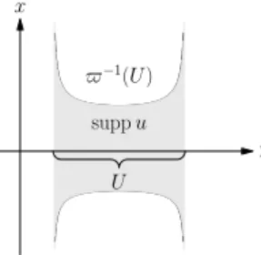
Let π :K2n∋ (x, ξ) +→ x ∈ Kn be the projection. Then the singular locus of M is defined by
It is an algebraic set ofKn since gr(M ) is homogeneous with respect to ξ. In particular, if M is holonomic, then Sing(M ) is an algebraic set of codimension≥ 1, or an empty set, since Char(M) is homogeneous with respect to ξ.
The set Char(M )\ ({0} × Kn) can be regarded as the subset of Kn × Pn−1(K), where Pn−1(K) is the (n − 1)-dimensional projective
space over K. Thus the problem of finding Sing(M) from Char(M) is completely solved by what is called the projective elimination theory, as is described in Chapter 8 of [6] in detail with a complete proof.
Proposition 3.16. Assume that K is an algebraically closed field of characteristic zero and set M = Dn/I with a left ideal I of Dn. Let
f1(x, ξ), . . . , fm(x, ξ) be polynomials homogeneous in ξ which generate
gr(0;1)(I). Let J
i be the ideal of K[x, ξ] generated by f1, . . . , fm with
the variable ξi replaced by 1. Set Ii = Ji∩ K[x]. Then Sing(M) is the
algebraic subset ofKn defined as the zeros of the ideal I
1∩ · · · ∩ In.
Thus we can compute Sing(M ) from Char(M ) by using appropriate Gr¨obner bases inK[x, ξ]; this fact was pointed out in [21], where it is also noticed that the characteristic variety as is defined here coincides with the analytic definition using the differential operators with analytic coefficients. Even if M is generated by more than one elements over Dn,
we can compute Char(M ) by using a Gr¨obner basis for a submodule of the free module (see [21] for details).
Example 3.17. Let
P = am(x)∂m+am−1(x)∂m−1+· · ·+a0(x) (ai(x)∈ K[x], am(x)̸= 0)
be a linear ordinary differential operator of order m ≥ 1 with x = x1
and ∂ = ∂1. Set M = D1/D1P . Then we have
Char(M ) ={(x, ξ) ∈ K2| σ(P )(x, ξ) = am(x)ξm= 0}
={(x, ξ) ∈K2| am(x) = 0} ∪ {(x, 0) | x ∈ K}.
Hence M is holonomic and Sing(M ) ={x ∈ K | am(x) = 0}, a point of
which is called a singular point of P .
Example 3.18. Let f be an arbitrary nonzero polynomial of x = (x1, . . . , xn). For each i = 1, . . . , n, ∂if = f ∂i + fi annihilates
the rational function 1/f , with fi:= ∂f /∂xi. Set M = Dn/I with
I := Dn∂1f +· · · + Dn∂nf.
For example, set n = 2 and f (x) = x3
1 − x22 which has a cusp
singularity at the origin. We can check that ∂1f and ∂2f are a (0;
1)-involutive basis of I. This gives
Char(M ) ={(x, ξ) ∈K4 | ξ1f (x1, x2) = ξ2f (x1, x2) = 0}
={(x, ξ) | x3
1− x22} ∪ {(x, ξ) | ξ = 0},
Sing(M ) ={(x1, x2)| x31− x22= 0}.
Hence the dimension of Char(M ) is 3, consequently M is not holo-nomic. In fact, I is much smaller than AnnD2(1/f ), which is generated
by 3x21∂2+ 2x2∂1 and 2x1∂1+ 3x2∂2+ 6. There is an algorithm to
com-pute AnnDn(1/f ) for an arbitrary polynomial f and Dn/AnnDn(1/f ) is
always holonomic (see [22], [29]).
Exercise 14. In the example above with n = 2 and f = x3 1− x22
(1) Verify that ∂1f and ∂2f are a (0; 1)-involutive basis of the ideal
I which they generate.
(2) Verify that P1:= 3x21∂2+ 2x2∂1 and P2:= 2x1∂1+ 3x2∂2+ 6
annihilate 1/f .
(3) Find a (0; 1)-involutive basis of J := D2P1+ D2P2 and verify
that D2/J is holonomic.
(4) Find the singular locus of D2/J.
Exercise 15. Find the characteristic variety and the singular locus of the left Dn-module M = Dn/(Dnx1+· · · + Dnxn).
Exercise 16. Let K = C and let f(x) ∈ C[x] = C[x1, . . . , xn].
Consider a C∞ function ef (x) on Rn. Set f
i = ∂i(f ) and M := Dn/I
with
I := Dn(∂1− f1) +· · · + Dn(∂n− fn).
(1) Show that I = AnnDne
f (x):={P ∈ D
n| P ef (x)= 0}.
(2) Show that HomDn(M, C∞(R
n)) ∼=Cef (x).
(3) Find the characteristic variety and the singular locus of M . 3.4. Equivalence of two definitions of holonomicity The purpose of this subsection is to prove Theorem 2.22 by using only basic tools in commutative algebra and Gr¨obner basis.
Definition 3.19 ([17]). A map ϕ fromN to {t ∈ R | t ≥ 0} is said to be of polynomial growth if there exists ν ∈ R such that ϕ(n) ≤ nν for
n≫ 0. Then we define the degree of ϕ by
deg ϕ = inf{ν | ϕ(n) ≤ nν for n≫ 0}. We set deg ϕ =∞ if ϕ is not of polynomial growth.