Title: Properties of variations in the periods of ring neural oscillators with noise Authors: Yo Horikawa and Hiroyuki Kitajima
Affiliation: Faculty of Engineering, Kagawa University, Takamatsu, 761-0396, Japan Corresponding author:
Yo Horikawa
Faculty of Engineering, Kagawa University, Takamatsu 761-0396, Japan Phone: +81-87-864-2211
Fax: +81-87-864-2262
E-mail address: horikawa@eng.kagawa-u.ac.jp
Abstract:
Effects of additive noise on a series of the periods of oscillations in unidirectionally coupled ring neural networks of ring oscillator type are studied. Kinematical models of the traveling waves of an inconsistency, i.e. the successive same signs in the states of adjacent neurons in the network, are derived. A series of the half periods in the network of N neuron is then expressed by the sum of N sequences of the N-1st-order autoregressive process, the process with the spectrum of exponential type and the first-order autoregressive process. Noise and the interaction of the inconsistency cause characteristic positive correlations in a series of the half periods of the oscillations. Further, an experiment on an analog circuit of the ring neural oscillator was done and it is shown that correlations in the obtained periods of the oscillations agree with the derived three expressions.
1. Introduction
We consider the following ring network of unidirectionally coupled neurons with sigmoidal input-output relations with additive noise.
dxn(t)/dt = -xn(t) + f(xn-1(t)) + σxwn(t) (x0 = xN, 1 ≤ n ≤ N (= 2M + 1 ≥ 3))
f(x) = tanh(gx) (g < -1/cos(π/N) < 0)
E{wn(t)} = 0, E{wn(t)wn’(t’)} = δnn’·δ(t - t’) (1)
where xn is the state of the nth neuron, N is the number of neurons, f(x) is the output function
of the neurons and g is the coupling gain. The neurons are unidirectionally coupled and the output of the Nth neuron is fed backed into the first neuron. The Gaussian white noise wn(t)
with the strength σx is added to each neuron independently. In the absence of noise, the
properties of the ring neural networks are as follows [1, 2, 12]. The origin xn = 0 (1 ≤ n ≤ N)
is globally stable when the absolute value of the coupling gain is less than unity (|g| < 1). When the couplings are excitatory (i.e. positive output of the nth neuron gives positive input to the n+1st neuron (g > 0)) and g > 1, the network has a pair of the non-zero stable steady states: (x1, x2, · · ·, xN ) = ±(xp, xp, · · ·, xp), xp = f(xp) > 0 and is bistable. When the
couplings are inhibitory (positive output gives negative input (g < 0)) and g < -1, the behavior of the network depends on the parity of the number of neurons. When the number of neurons is even (N = 2M), the network is bistable: (x1, x2, · · ·, xN ) = ±(xp, -xp, · · ·, -xp), in which
the signs of the states of neurons change alternately. When the number of neurons is odd (N = 2M + 1 ≥ 3) and the coupling gain is less than the value of the Hopf bifurcation point (g < -1/cos(π/N)), however, the network is qualitatively the same as a ring oscillator and shows stable oscillations. The ring oscillator is a closed loop of inverters and is widely used as a variable-frequency oscillator in analog and digital circuits [10]. The mechanism of the oscillations is qualitatively simple. Let the state x1 of the first neuron be positive. Its inverting
output f(x1) < 0 (g < 0) is transmitted to the second neuron, and so on. The Nth neuron then
gives negative input to the first neuron, which makes the state of the first neuron negative. This inconsistency propagates in the direction of the coupling. When N = 3, for instance, the states of neuron changes as (x1, x2, x3): (+, -, +) → (-, -, +) → (-, +, +) → (-, +, -) → ···. The
state of each neuron then oscillates in the form of a rectangular wave.
Such ring networks of neurons in the absence of noise have been widely studied from the viewpoint of the dynamics of neural networks [1, 12], for recurrent neural networks [2] and as cyclic feedback systems [7] so that their various properties have been proven. The discrete systems of them have multiple stable orbits [27] and the networks with delays cause various spatio-temporal patterns [9, 21, 29] and long lasting transient oscillations [3, 4, 30]. Further, it was recently shown that the ring networks even without delays cause long lasting transient oscillations [18, 22, 24, 25] and the duration increases exponentially with the number of neurons [19, 20].
In this study we consider effects of temporal noise on the ring neural networks of ring oscillator type, in which stable oscillations exist. Although it is known that there are clock jitter and phase noise in ring oscillators and they have been studied [13, 25], the properties shown in this paper has not been shown as far as the authors know. Expressions for variations and correlations in the periods of the oscillations due to the noise are then obtained with the kinematical descriptions of the traveling waves in the networks which result in the oscillations of the state of neurons. In Sect. 2, a series of the half periods of the oscillations is formulated as a discrete time series and is expressed as the sum of the autoregressive process.
In Sect. 3, changes in the half periods are formulated with a differential equation model and correlations in a series of the half periods with power spectra of exponential type are derived. The derived expressions for a series of the half periods agree with simulation results. Further, the results of an experiment on an analog circuit of the ring neural oscillator are shown in Sect. 4. Finally, conclusion and discussion are given in Sect. 5.
2. Discrete process model
Let the number of neurons be odd: N = 2M + 1 ≥ 3 with negative coupling gain less than the Hopf bifurcation point: g < -1/cos(π/N) < 0 in Eq. (1). The network shows a stable oscillation, which corresponds to the ring oscillator. As mentioned in Sect. 1, there is one inconsistency in the signs of the states of neurons, i.e. the two successive same signs, and it rotates in the direction of the coupling as (x1, x2, · · ·, xN): (+, -, +, +, -, +, -, · · ·, -) → (+, -, +,
-, -, +, -, · · ·, -) → (+, -, +, -, +, +, -, · · ·, -) → ···. The oscillation is this traveling wave of the inconsistency. We consider variations in the half periods (i.e. the pulse width) of the stable oscillation caused by the noise. The half period is the interval of the passing time of the successive inconsistencies at one neuron. The inconsistency rotates the network one time in the half period and then the period of the oscillation is its double.
In this section, we derive an expression for a series of the half periods of the oscillations as a discrete time series. We here replace f(x) with the following sign function, which corresponds to the limit of the coupling gain g → - ∞.
sgn(-x) = -1 (x ≥ 0)
= 1 (x < 0) (2)
Let tj(n) be the time at which the state xn of the nth neuron be zero at jth time, i.e. the time of jth occurrence of xn = 0. We define the propagation time ∆tj(n) of the inconsistency at the nth
neuron at jth time by
∆tj(n) = tj(n) - tj(n - 1) (1 ≤ n ≤ N, tj(0) = tj-1(N)) (3)
That is, the propagation time is time required for the propagation over one unit distance (one neuron). In the absence of the noise, the propagation time m(∆t) (= ∆tj(n), for all n and j) of the inconsistency and the half period Tm of the stable oscillation are constant and given by the
following equations [2].
xmax = -(xmax + 1)exp(-Tm) + 1 (xmax > 0)
m(∆t) = log(xmax + 1), Tm = Nm(∆t) (4)
The value xmax is the maximum value xn(tj-1(n - 1)) of the states of the neurons at the time when the states of the preceding neurons cross zero (xn-1 = 0) from negative to positive. The
first equation in Eq. (4) is derived from the condition: xn(tj(n - 1)) = xn(tj-1(n - 1) + Tm) = -xn(tj-1(n - 1)), and m(∆t) is the solution of the equation: xn(tj(n - 1) + m(∆t)) = (xmax + 1)exp(-m(∆t)) - 1 = 0.
The propagation time varies in the presence of noise. Let the state xN of the Nth neuron
change from positive to negative at t = tj-1(N) and be negative until t = tj(N). When the sign
function (Eq. (2)) is used for f(x), changes in the state x1(t) of the first neuron results in the Ornstein-Uhlenbeck (OU) process in the interval (tj-1(N), tj(N)) as
dx1(t)/dt = -x1(t) + 1 + σxw1(t), x1(tj(1)) = 0 (tj-1(N) = tj(1) - ∆tj(1) < t < tj(N)) (5)
The probability density function of x1(tj(N)) at t = tj(N) is then Gaussian [8]. The mean
m(x1(tj(N))) is then given by the solution for σx = 0 as m(x1(tj(N))) = 1 - exp[-(tj(N) - tj(1))] = 1 - exp(-
∑
= ∆ N n j n t 2 ) ( ) ≈ 1 - exp[-(N - 1)m(∆t)]∏
= ∆ − N n j n t 2 )) ( ' 1 ( ≈xmax+ exp[-(N - 1)m(∆t)]∑
= ∆ N n j n t 2 ) ( ' ∆t’j(n) = ∆tj(n) - m(∆t) (6)where we use the condition x1(tj(1)) = 0 and approximate x1(tj-1(N)) by -xmax.
The variance σ2(x1(tj(N))) is approximated by the variance at the mean elapsed time m(tj(N) -
tj(1)) = (N - 1)m(∆t) as [8]
σ2(x1(tj(N)) ≈ σ2(x1(tj(1) + (N - 1)m(∆t)))
= σx2/2·{1 - exp[-2(N - 1)m(∆t)]} (7)
The propagation time ∆tj+1(1) of the inconsistency at the first neuron at j+1st time is given by
the first passage time (FPT) of x1 from x1(tj(N)) to 0 as
dx1(t)/dt = -x1(t) - 1 + σxw1(t), x1(tj(N) + ∆tj+1(1)) = 0 (t ≥ tj(N)) (8)
When the variance of the noise is small (σx2 « 1), the mean of the FPT is approximated by
m(∆t) in the absence of noise. Hence,
∆tj+1(1) = log[1 + x1(tj(N))] + σ(∆t)wj+1(1)
= log[1 + m(x1(tj(N))) + σ(x1(tj(N)))wj’] + σ(∆t)wj+1(1)
= log{1 + xmax+ exp[-(N - 1)m(∆t)]
∑
= ∆ N n j n t 2 ) ( ' + σ(x1(tj(N)))wj’} + σ(∆t)wj+1(1) ≈ m(∆t) + exp(-Nm(∆t))∑
= ∆ N n j n t 2 ) ( ' + σt’wj’ + σ(∆t)wj+1(1) σ2(∆t) ≈ σx2/2·{1 - exp[-2m(∆t)]}σt’2 = exp(-2m(∆t))σ2(x1(tj(N))) ≈ σx2/2·{1 - exp[-2(N - 1)m(∆t)]}exp(-2m(∆t)) (9)
where wj+1(1), wj’, wj+1 are the Gaussian white noise, e.g. E{wj(n)} = 0, E{wj(n)wj’(n’)} =
δj,j’δnn’. The variations in ∆tj+1(1) consist of two factors; σ(∆t)wj+1(1) is due to the noise
σxw1(t) in Eq. (8) and σt’wj’ is due to the variation in x1(tj(N)). Here the variance σ2(∆t) is
approximated by that of x1(tj(N) + ∆tj+1(1)). That is, the probability density function of
x1(tj(1)) is Gaussian and the probability density function of the FPT is approximated by the
the slope of the trajectory at x1(t) = 0 in the absence of noise is minus unity (dx1/dt|x1 = 0 = -1).
The variance of x1(tj(N) + ∆tj+1(1)) is then approximated by letting x1(tj(N)) = xmax and ∆tj+1(1)
= m(∆t).
A series of the propagation times ∆tj(n) is then expressed by the N-1st-order autoregressive
(AR) process with the same positive weights exp(-Tm) as
∆tj+1’(1) ≈ exp(-Tm)
∑
= ∆ N n j n t 2 ) ( ' + σtwj+1, ∆t’j(n) = ∆tj(n) - m(∆t) σt2 = σt’2 + σ2(∆t)= σx2/2·[1 - exp[-2m(∆t)] + {1 - exp[-2(N - 1)m(∆t)]}exp(-2m(∆t))] (10)
The power spectrum is given by
S(ω; ∆tj(n)) = σt2/|1 -
∑
− = ω − − 1 1 ) i exp( ) exp( N n m n T |2 (-π ≤ ω ≤ π) (11)The half period Tj is the sum of the propagation times of N neurons (Tj =
∑
= ∆ N n j n t 1 ) ( ). It is
given by making a series
∑
= + ∆ N m j n m t 1 )
( of the sums of the propagation times of the successive N neurons and then doing downsampling by a factor N of them. The power spectrum S(ω; Tj) of a series of the half period Tj is obtained by N times folding at ω = π/N
after multiplying S(ω; ∆tj(n)) by |
∑
− = ω − 1 0 ) i exp( N n n |2. S(ω;∑
= + ∆ N m j n m t 1 ) ( ) = S(ω; ∆tj(n))|∑
− = ω − 1 0 ) i exp( N n n |2 S(ω; Tj) = [ ( / ; ( )) 1∑
= + ∆ ω N m j m n t N S + ((2 )/ ; ( )) 1 2 / 1∑
∑
= = + ∆ ω − π N m j N k m n t N k S + ((2 )/ ; ( )) 1 2 / ) 1 ( 1∑
∑
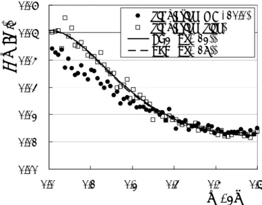
= − = + ∆ ω + π N m j N k m n t N k S ]/N (12)Figure 1 shows the power spectra S(ω; Tj) of a series of the half periods in the ring network
of three neurons (N = 3) in the presence of noise of σx = 0.1. Plotted are estimates with the
average of two hundred spectra with 128 point FFT of 25600 half periods obtained with computer simulation of Eq. (1) with g = -10.0 (closed circles) and with the sign function (Eq. (2)) (open squares). A time step for numerical calculation is 0.001. Equation (12) is also plotted with a solid line. The values of the parameters for N = 3 are:
xmax = (-1 + 51/2)/2 ≈ 0.618, m(∆t) = log((1 + 51/2)/2) ≈ 0.481,
Tm = log(2 + 51/2) ≈ 1.44, exp(-Tm) = (xmax +1)-3 = -2 + 51/2 ≈ 0.236 (in Eq. (4)),
= 2(-2 + 51/2)σx2 ≈ 0.472σx2 (in Eq. (10)) (13)
The expression with Eq. (12) (solid line) agrees with the simulation results with the sign function (open squares), while the power of the simulation results with the sigmoidal function with g = -10.0 (closed circles) is slightly smaller than them. The power spectra increase in the low frequency region and thus the noise causes positive correlations in a series of the half periods. However, the value of the weights of the AR process decreases exponentially with the number N of neurons. The correlations due to the noise are then considerable only for small N. Decreases in the variations in the half periods for the sigmoidal function f(x) = tanh(gx) might be contrary to intuition but are explained as follows. The FTP of x1 in Eq. (8)
with f(x) is the time for changes in x1 from f(xN) to f -1(x2) and the length reduces to |f(xN) - f
-1(x
2)| (< xmax). This reduction and shift in the length of FPT makes the variance of the
propagation time smaller, though changes in x1 is slower owing to |f(x)| < 1 so that the mean
propagation time increases about to 0.51 (m(∆t) ≈ 0.481).
3. Differential equation model
In this section, we derive a differential equation model for changes in the half periods and derive their properties. From Eq. (9), the propagation time ∆tj+1 of the j+1th passing of the
inconsistency at the nth neuron is expressed with the half period Tj by
∆tj+1 ≈ log{1 + xmax+ exp[-(N - 1)m(∆t)][(N - 1)/N]T’j} + σt’wj’ + σ(∆t)wj+1
≈ m(∆t) - exp(-Tm)[(N - 1)/N]Tj’ + σtwj+1
σt2 = σt’2 + σ2(∆t), Tj = tj - tj-1, Tj’ = Tj - Tm (14)
where the neuron number is omitted since it is arbitrary. The coefficient of T’jis multiplied by
(N - 1)/N since ∆tj in Tj must be excluded since it does not contribute to changes in x1(tj+1)
according to the derivation of Eq. (9). Then the changes in the half period Tj at the location l
in the network is expressed as dTj(l)/dl = d(tj - tj-1)/dl ≈ ∆tj - ∆tj-1
≈ β(Tj - Tj-1) + σt(wj - wj-1)
β = exp(-Tm)·(N - 1)/N, Tj(0) = Tj-1(N) (15)
where l corresponds to the neuron number but is continuous in 0 ≤ l ≤ N. Following [15], the z transform ZT of Tj is given by dZT(l)/dl = β(1 - z-1)ZT(l) + (1 - z-1)Zw(l) ' d ) ' ( )] ' )( 1 ( β exp[ ) 1 ( ) 0 ( ] ) 1 ( β exp[ ) ( 1 0 1 1 l Z z z l l Z l l z l Z w l T T = − − + − −
∫
− − − ZT(0) = z-1ZT(N) (16)where Zw(l) is the z transform of the noise σt(wj - wj-1) and ZT(l) is derived from the first and third equations. Hence the power spectrum S(ω) of Tj is obtained as
S(ω) = E{|ZT(N)|2 z = exp(iω)} iω -iω 2 0 2 | )] e 1 ( β exp[ e 1 | / d ))] ω cos( 1 )( ( β 2 exp[ )) ω cos( 1 ( 2 − σ − − − − = t
∫
N N l l N = σt2/β·{exp[2βN(1 - cos(ω))] - 1}/{1 + exp[2βN(1 - cos(ω))] - 2exp[βN(1 - cos(ω))]cos[ω - βNsin(ω)]} (17) The power spectrum is of exponential form. It increases in a low frequency region since S(0) = σt2N/(1 - βN)2 is larger than S(π) ≈ σt2N and S(ω) = σt2N for β = 0. Equation (17) for N = 3 is
also plotted with a dashed line in Fig. 1, where β = 2/3·(-2 + 51/2) ≈ 0.157. It hardly differs from Eq. (12) and agrees with the simulation results with the sign function.
When |βN| < 1, a series of the half periods is further expressed as the first-order AR process as follows. Tj(N) = tj(N) - tj-1(N) = Tj l tnj l N d ) ) ( β ( 0 +σ
∫
≈ βN/2·(Tj-1(N) + Tj(N)) + σTwj Tj(N) = φ1Tj-1(N) + σTwj φ1 = βN/(2 - βN), σT2 = σt2N/(1 - βN/2)2 (18)where the trapezoidal rule is used for the estimation of the integral in the first equation to derive the second equation. The weight φ1 is positive and the power spectrum S(ω) and the
autocovariance function γk of a series of the half periods is given by
S(ω) = σT2/(1 - 2φ1cos(ω) + φ12)
γk = E{(Tj(N) - Tm)(Tj-k(N) - Tm)} = σT2/(1 - φ12)·φ1k (k ≥ 0) (19) The values of the parameters of the first-order AR process for N = 3 are: φ1 = (-1 + 51/2)/4 ≈
0.309, σT2 = 3/4·(1 + 51/2)σx2 ≈ 2.43σx2. The power spectrum S(ω) in Eq. (19) also agrees with
Eqs. (12) and (17) (not shown in Fig. 1).
4. Circuit experiment
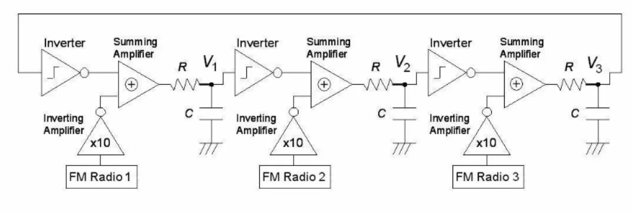
In this section, we show the results of an experiment with an analog circuit for the ring neural networks. Figure 2 shows an analog circuit of the ring neural oscillator of three neurons with noise. It was made with TC4049 for inverters and operational amplifiers RC4558 for inverting and summing amplifiers. The sigmoidal function f(x) = tanh(gx) is replaced with the step function of the inverter: Vout = 0V for Vin > 2.5V, Vout = 5V for Vin <
2.5V with the supply voltage 5V. The supply voltage for the operational amplifiers is 12V, and C = 1µF, R = 10kΩ, (time constant: CR = 10ms) were used. Noise sources were three untuned FM radios. It was checked that these noise sources are hardly correlated with each other.
We measured the half periods of the oscillations by recording the times at which the voltage V1 at the first node crosses the threshold voltage 2.5V of the inverters. We then
obtained and used a series of the periods (the sum of the successive two half periods) of the oscillations. It is because small biases in the supply voltage and offset voltages of the inverters cause considerable differences between the averages of the positive and negative half periods. (The terms of positive and negative correspond to the signs of the states of the neuron, hence the voltage in the half periods are over and below the threshold 2.5V, respectively.) They cause alternate variations in a series of the half periods and apparent large negative correlations.
The power spectrum S(ω; Tpj) of a series of the periods Tpj = T2j + T2j+1 is given by doing
downsampling by a factor two of a series of the sums of the successive two half periods as S(ω; Tpj) = [1 + cos(ω/2)]S(ω/2; Tj) + [1 + cos(π - ω/2)]S(π - ω/2; Tj) (20)
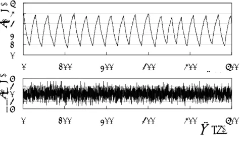
Figure 3 shows an example of time series of the voltage V1 (upper panel) at the first node and
the noise voltage Vw (lower panel) in the analog circuit. The mean and SD of the voltages of
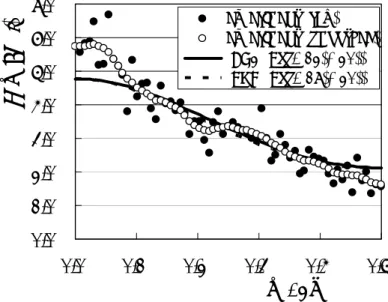
the noise measured at the outputs of the inverting amplifiers were 0.0V and 1.53V respectively. The noise varies the waveform of the voltage V1. Figure 4 then shows the power
spectra S(ω; Tpj) of a series of the periods Tpj. Plotted are estimates with the average of 40
spectra with 128 point FFT of 5120 periods obtained with the experiment (raw (closed circles) and smoothed with triangle windows (open circles)), and Eq. (20) with Eq. (12) for the second-order AR process (solid line) and with Eq. (17) for the differential equation model (dashed line). The value of the variance σt2 in Eqs. (12) and (17) was estimated with the
variance σ2(Tj) = E{(Tj - Tm)(Tj - Tm)} ≈ 1.26ms2 of the measured half periods Tj by σt2 =
σT2(1 - βN/2)2/N = σ2(Tj)(1 - φ12)(1 - βN/2)2/N ≈ 0.222. The power spectra increase in the low
frequency region and a series of the periods is positively correlated though the correlations are smaller than those in a series of the half periods. The expressions with the second-order AR process and of exponential type agree about with the result of the experiment though they are slightly smaller in the low frequency region.
5. Conclusion and discussion
The kinematical description of the traveling waves of the inconsistency in the rings of unidirectionally coupled neurons in the presence of additive noise was derived. In the ring network with odd numbers of neurons and sufficiently large inhibitory couplings, there is one traveling wave at which there is the inconsistency in the signs (the two successive same signs) of adjacent neurons. The resulting oscillation is stable and the corresponding electronic circuit is known as the ring oscillator. It was shown that the noise causes the positive correlations in a series of the periods of the oscillations. A series of the half periods is expressed by the sum of the successive N propagation times, which is expressed by the N-1st-order AR process with the same positive weights, where N is the number of neurons. It is also described by the differential equation model and the power spectrum is expressed in the form of the exponential function of frequency. Further, it is expressed by the first-order AR process with the positive weight. These three expressions agree with the results of the computer simulation and experiment. A series of the half periods is positively correlated owing to the interaction with the previously passing inconsistency in Eq. (15). The speed of the inconsistency increases when the elapsed time after the preceding passage decreases since the interaction is attractive (β > 0). The successive half periods then tend to remain long or short depending on the preceding ones, which results in positive correlations.
When there are two or more inconsistencies in the ring neural network, the inconsistencies interact with each other attractively. Smaller distances between them decrease and the inconsistencies collapse and disappear even in the absence of noise. Finally, one
inconsistency remains when the number of neurons is odd, which is a stable oscillation, while no inconsistencies remain and the network reaches one the two stable states when the number of neurons is even. When the number of neuron is large, the interaction is expressed with the exponentials of the distances lj (the number of neurons) between the adjacent inconsistencies
as [19, 20]
dlj/dt ≈ 1/(log2)2·[exp(-log2·lj-1) - exp(-log2·l j)] (21)
The interaction is exponentially small with the distances, hence the number of neurons, and changes in the distances are exponentially slow. Transient states then become exponentially long as the number of neurons increases. It was shown that the exponentially long transient oscillations in the networks of even numbers of neurons are two inconsistencies traveling in the networks and the properties of the duration of the oscillations were derived [18 - 20, 22, 24, 25]. It is also known that the movement of fronts or kinks in bistable reaction-diffusion equations is expressed in the same form as Eq. (21) and the movement is exponentially small [5, 6, 23]. The duration of the transient fronts then increases exponentially with the length of domains. It was shown that the properties of the duration of the fronts are similar to those of the duration of the oscillations in the ring neural networks [17].
It is also known that similar interactions exist in a car-following model in traffic flow problems [11, 31] and spike propagation in excitable media [26, 28]. In these cases the interaction is mainly repulsive contrary to the ring neural networks and the bistable reaction-diffusion equations. In excitable media, e.g. a nerve fiber, the propagation speed of a spike decreases in the refractory period. It is known that the interaction between the spikes then smooths the interspike intervals in a spike train propagating in a nerve fiber and cause positive correlations in a series of the interspike intervals [14 - 16]. It has been shown, however, that the interaction causes negative correlations in the intervals in a spike rotating in a ring nerve fiber with noise [15]. It is of interest that the correlations caused by the same interaction differ between line and ring media.
When a signal is added to one end of an open chain or array of the neurons, rectangular pulses switching positive and negative signs can be generated and propagated toward the other end. The chain network is then regarded as a transmission line of the signals. Each pulse interacts with the preceding one attractively in the chain networks through Eq. (15). It is then expected that variations in the pulse widths increase and the pulse sequence becomes negatively correlated during propagation. The sign of correlations in the pulse sequences in the chain networks is opposite to that in the half periods in the ring networks. Further, small pulses disappear and the adjacent pulses merge during propagation when the number of neurons is large. These changes result in modulations of the signals and their properties are now under study.
References
[1] S. Amari, Mathematics of Neural Networks (in Japanese) (Sangyo-Tosho, Tokyo, 1978). [2] A. F. Atiya and P. Baldi, Oscillations and synchronizations in neural networks: an exploration of the labeling hypothesis, Int. J. Neural Systems 1 (1989) 103-124.
[3] K. L. Babcock and R. M. Westervelt, Dynamics of simple electronic neural networks, Physica D 28 (1987) 305-316.
[4] P. Baldi and A. F. Atiya, How delays affect neural dynamics and learning, IEEE Trans. Neural Networks 5 (1994) 612-621.
[5] J. Carr and R. L. Pego, Metastable patterns in solutions of u = εu - f(u), Commun. Pure Appl. Math. 42 (1989) 545-576.
[6] S. Ei and T. Ohta, Equation of motion for interacting pulses, Phys. Rev. E 50 (1994) 4672-4678.
[7] T. Gedeon, Cyclic Feedback Systems,Memoirs of the American Mathematical Society (American Mathematical Society, 1998).
[8] N. S. Goel and N. Richter-Dyn, Stochastic Models in Biology (Academic Press, 1974). [9] S. Guo and L. Huang, Pattern formation and continuation in a trineuron ring with delays, Acta Mathematica Sinica 23 (2007) 799-818.
[10] G. Gutierrez, Variable-frequency oscillators, in: J. G. Webster, ed., Wiley Encyclopedia of Electrical and Electronics Engineering, vol. 23 (John Wiley, 1999) 75-84.
[11] R. Haberman, Mathematical Model: Traffic Flow (Prentice Hall, 1977).
[12] M. H. Hirsh, Convergent activation dynamics in continuous time series, Neural Networks 2 (1989) 331-349.
[13] A. Hajimiri, S. Limotyrakis and T. H. Lee, Jitter and phase noise in ring oscillators, IEEE J. Solid-State Circuits 34 (1999) 790-804.
[14] Y. Horikawa, Spike propagation during the refractory period in the stochastic Hodgkin-Huxley model, Biol. Cybern. 67 (1992) 253-258.
[15] Y. Horikawa, Noise effects on spike propagation during the refractory period in the FitzHugh-Nagumo model, J. Theoretical Biology 162 (1993) 41-59.
[16] Y. Horikawa, A spike train with a step change in the interspike intervals in the FitzHugh-Nagumo model, Physica D 82 (1995) 365-370.
[17] Y. Horikawa, Duration of transient fronts in a bistable reaction-diffusion equation in a one-dimensional bounded domain, Phys. Rev. E 78 (2008) 066108/1-10.
[18] Y. Horikawa and H. Kitajima, Experiments on transient oscillations in a circuit of diffusively coupled inverting amplifiers, in: M. Tacano, et al. eds., Noise and Fluctuations: 19th International Conference on Noise and Fluctuations; ICNF 2007, Conference Proceedings Series 922 (AIP, New York, 2007) 569-572.
[19] Y. Horikawa and H. Kitajima, Properties of the duration of transient oscillations in a ring neural network, in: Proc. 2008 Int. Symp. on Nonlinear Theory and its Applications (NOLTA 2008) (2008) 520-523.
[20] Y. Horikawa and H. Kitajima, Duration of transient oscillations in ring networks of unidirectionally coupled neurons, Physica D 238 (2009), pp. 216-225.
[21] C. Huang, et al., Global exponential periodicity of three-unit neural networks in a ring with time-varying delays, Neurocomputing 71 (2008) 1595–1603
[22] T. Ishii and H. Kitajima, Oscillation in cyclic coupled neurons, in: Proc. 2006 RISP Int. Workshop on Nonlinear Circuits and Signal Processing (NCSP2006) (2006) 97-100.
[23] K. Kawasaki and T. Ohta, Kink dynamics in one-dimensional nonlinear systems, Physica 116A (1982) 573-593.
[24] H. Kitajima and Y. Horikawa, Oscillation in cyclic coupled systems, in: Proc. 2007 Int. Symp. on Nonlinear Theory and its Applications (NOLTA 2007) (2007) 453-456.
in: Proc. 2006 Int. Symp. on Nonlinear Theory and its Applications (NOLTA 2006) (2006) 623-626.
[25] J. A. McNeill, Jitter in ring oscillators, IEEE J. Solid-State Circuits 32 (1997) 870-879. [26] R. N. Miller and J. Rinzel, The dependence of impulse propagation speed on firing frequency, dispersion, for the Hodgkin-Huxley model, Biophys. J. 34 (1981) 227-259.
[27] F. Pasemann, Characterization of periodic attractors in neural ring networks, Neural Networks 8 (1995) 421-429.
[28] J. Rinzel, Impulse propagation in excitable systems, in: W. E. Stewart, et al. eds., Dynamics and Modelling of Reactive Systems (Academic Press, New York, 1980) 259-291. [29] X. Xu, Complicated dynamics of a ring neural network with time delays, J. Phys. A 41 (2008) 035102 (23pp).
[30] K. Pakdaman, C. P. Malta, C. Grotta-Ragazzo, O. Arino and J.-F. Vibert, Transient oscillations in continuous-time excitatory ring neural networks with delay, Phys. Rev. E 55 (1997) 3234-3248.
Figure captions
Fig. 1. Power spectra S(ω) of a series Tj of the half periods in the ring neural oscillator of
three neurons (N = 3) in the presence of noise of σx = 0.1. Estimates with the results of
computer simulation of Eq. (1) with g = -10.0 (closed circles) and with the sign function (Eq. (2)) (open squares), Eq. (12) (solid line) and Eq. (17) (dashed line).
Fig. 2. Analog circuit of the ring neural oscillator of three neurons with noise.
Fig. 3. Time series of the voltage V1 (upper panel) at the first node and the noise voltage Vw
(lower panel) in the analog circuit.
Fig. 4. Power spectra S(ω; Tpj) of a series of the periods Tpj in the analog circuit. Estimates
with the results of the experiment (closed and open circles), and Eq. (20) with Eq. (12) (solid line) and with Eq. (17) (dashed line).
Fig. 1. Power spectra S(ω) of a series Tj of the half periods in the ring neural oscillator of
three neurons (N = 3) in the presence of noise of σx = 0.1. Estimates with the results of
computer simulation of Eq. (1) with g = -10.0 (closed circles) and with the sign function (Eq. (2)) (open squares), Eq. (12) (solid line) and Eq. (17) (dashed line).
0.00 0.01 0.02 0.03 0.04 0.05 0.06 0.0 0.1 0.2 0.3 0.4 0.5 ω/2π
S
(ω ;T
j) simulation (g = -10.0)simulation (sign)
AR2 (Eq. (12)) EXP (Eq. (17))
Fig. 3. Time series of the voltage V1 (upper panel) at the first node and the noise voltage Vw
(lower panel) in the analog circuit. 0 1 2 3 4 5 0 100 200 300 400 500 t (s)
v
1 (V ) -6 -30 3 6 0 100 200 300 400 500t
(ms)v
n (V)Fig. 4. Power spectra S(ω; Tpj) of a series of the periods Tpj in the analog circuit. Estimates
with the results of the experiment (closed and open circles), and Eq. (20) with Eq. (12) (solid line) and with Eq. (17) (dashed line).
0.0 1.0 2.0 3.0 4.0 5.0 6.0 7.0 0.0 0.1 0.2 0.3 0.4 0.5
ω/2π
S
(ω
;
Tp
j)
experiment (raw) experiment (smoothed) AR2 (Eqs. (12), (20)) EXP (Eqs. (17), (20))Vitae
Yo Horikawa is a professor in the Faculty of Engineering at Kagawa
University, Japan. He received B. Eng., M. Eng. and Ph. D. (Eng.) degrees in mathematical engineering and information physics from the University of Tokyo in 1983, 1985 and 1994 respectively. His research interests include signal processing in excitable media and statistical pattern recognition.
Hiroyuki Kitajima received the B.Eng. and M.Eng., and Dr. Eng.
degrees from The University of Tokushima, Tokushima, Japan, in 1993, 1995, and 1998 respectively. He is now an Associate Professor, Dept. of Reliability-based Information Systems Engineering, Kagawa University, Japan. He is interested in bifurcation problems.