An Approximation Formula for the Mean Waiting Time of an M/G/ c Queue

Journal of the Operations Research Society of Japan

Vo1.20, No.3, September, 1977

AN APPROXIMATION FORMULA FOR THE MEAN

WAITING TIME OF AN

M/G/c QUEUE

YUKIO T AKAHASHI

Tohoku University

(Received October 18, 1976; Revised March 25, 1977)

Abstract An approximation formula for the mean waiting time of an M/G/c queue is proposed. It estimates the mean waiting time from a moment of order Q~ 2, rather than the second moment! of the service distribution. To-gether with the Lee & Longton's formula [I] and the Page's formula [2], it was numerically tested on a variety of cases, and the test shows that the new formula is generally better than the previous two formulas, especially for queues with mixtures of Erlang distributions as the service distribution. A similar approximation formula for the variance of the waiting time is also proposed.

1. Introduction

Many approximation formulas for the mean waiting time of an M/C/c queueing system have been proposed by Lee & Longton [1], Page [2] and other authors. Most of them estimate the mean waiting time EC(W) from the 2nd moment b

Z of the service distribution using the values of the mean waiting times EM(W) and ED(W) of the corresponding M/M/c and M/D/c queueing systems with the same mean service time and the same traffic intensity. For example, the Lee & Longton's formula is

(1.1)

and the Page's formula is

(1. 2)

where

?

c

(W) b. is the ith

'&

The author tested b 2 _{I ) E (W)}

+

(2 -b 2 _E

_UI)

b2

M

,

b l 2 D I

moment of the service distribution.

the above two approximations on a variety of cases designated in Table I in Section 3. The result of the test, which is summa-rized in Table 2 in Section 3, shows that the~e approximations are fairly good for queueing systems with convolutions of Erlang distributions as the service distribution. But for some queueing systems with mixtures of Erlang distributions, they are not good. It seems that the use of the 2nd moment causes the unfitness. As will be discussec in the next section, the 2nd moment is not suitable for estimating the mean waiting time of a multi-channel queueing system, especially of a system with IQW traffic intensity. A moment:

of lower order than 2 will be rather adequate to estimate it.

In this paper we explore a new approximation formula which estimates the mean waiting time EC (W) from a moment b

a of order a < 2 of the service

distribution. From several natural conditions stated in the next section, we can derive the following approxima tion formula.

b I

(1. 3) _EC (W) a a-I (W)

b a ED

,

1

where a is the unique positive number suc:h that

(1.4)

1

a-I

rea+1» ED (W) ,

where r(z) is the gamma function. This formula was also tested in the cases designated in Table 1. The relative error has been less than 10% in every case in the test, and in most cases this approximation has been better than the previous two approximations, especially in cases of mixture type service distributions.

Similarly we can derive an approximation formula for the variance

Vc (W) of the waiting time. Let V

M (f.f) and the waiting times of the corresponding M/11/e

VD (W) be the variances of and M/D/e queueing systems with the same mean service time and the same traffic intensity, and

B

be the unique positive number such that

152 Y. TakiJhashi 2 (1. 5)

v

(W) - (E (/» 2 M M

(f(B+l»B-l

{VD(W) - (ED(W»2} Then VC(W) is approximated by 2 (1. 6)

~j-b B 1

) B-1

{VDU>') - (E D(W»2}

+

(;G(W»2

The relative error of the approximation has been less than 21% in every case designated in Table 1.

Tables of a,

B,

E (W),

M and

are presented in Appendix, together with some notes on calculations of and

2. A New Approximation Formula for the Mean Waiting Time

The purpose of this section is to show the derivation process of the new approximation formula (1.3) from several conditions. Let us consider a multi-channel queueing system M/G/e In the system, customers arrive at a serviC0 facility with (? channels in parallel via a Poisson process with rate ' \ .

If all channels are busy, the customers form a single queue and are served in order of arrival. The service times are independent random variables subject-ing to a distribution function G(.r) Let b be the moment of order y

y

of the distribution G, and p

=

,\bl/e the traffic intensity. We denote by

EC(W) the mean waiting time in the steady-state.

First we show a reason for considering an approximation formula which depends on b

a for some a ~ 2 rather than b 2 Let L be the total number of customers being served or waiting in the queue. Since

00

(2.1)

i

L

nP{L

n=l

,. + n} ,

i f p is sufficiently small, EGO>')

As p tends to zero, P {L

=

e + I}

is approximated by

.!.

P {L = e + 11 .

,\

is asymptotically equal to the conditional probability of the same event conditioned that the services of e customers being served have begun with their arrivals. Hence, when ,\ tends to zero,

(2.2) where (2.3) Hence,

o

I f c = 1) , P {L

=

c+l}

=

J:

xK(x)G(;r)dx

+

o(A)

G(x)

=

1 - C(x) and K(x) is a function given by

K(x)

C

G(x 2)dx2

r

C(x 3)dx3

r

C(x )dx c c x₂ x c_l E (VI) C K(x)

is proportional to the integral in (2.2) for sufficiently small in the integrand is a constant function (this is the case if then the integral is proportional to b

2

,

and it becomes reasonable to estimate ECOI) from b However, i f c > 1 K(x) is a

non-2

increasing function vanishing at infinity. So, the masses of C at large x's less contribute to the integral, and i t seems rather adequate to estimate

EC(1) from a moment of lower order than 2 .

Next, associated with the above queueing system, let us consider another queueing system with c channels, a Poisson arrival process with rate

A' =

Alp,

and a service distribution function (2.4) C I (x) = q + [}C(x) , x~O,

where p and q are positive numbers such that p + q

=

1 the mean waiting time of the new system and by b I

Y

We denote by the moment of order y of C' Then b'y

=

pb_y ' and the traffic intensity of the new system is the same as that of the original system. This system is considered that customers requiring service times equal to zero are added to the original system in a random fashion. So both queueing systems have the same waiting time distribution, especially the same mean waiting time, Le.,

(2.5)

It is desirable that approximation formulas have the corresponding property to (2.5). The Lee & Longton's for-mula (1.1) satisfies this property, but the Page's formula (1.2) does not.

There is another property which shoulc be satisfied by approximation formulas. If the time scale of a queueing system is changed, then the mean waiting time of the system changes proportionally to it. To say more pre-cisely, let EC*(rv) be the !'lean waiting time of a queueing system formed from the qlleucing system under condisderation by changing the time scale so that the arrival rate ~* = ~/O and the service distribution function

154 Y. Takahashi

c* (x) = C(x / 8 ) . Then E

C* (W) = 8E C (W). This property should be retained·

by approximation formulas. Both the Lee & Longton's formula and the Page's formula satisfy this property.

Now we shall consider a new approximation formula for depends on the service distribution only through b

l and

EC(W) which

b for some

a a < 2 and which satisfies the two properties stated above. Let

A(b

l , b) be the approximation formula.

A a

Then from the first property

EC(W) corresponding to (2.5)

(2.6)

and from the second property EC*(W)

=

8EC(W) ,

(2.7)

It can be proved that if (2.6) and (2.7) hold for any possible values of b l ' b p and 8 , then the function A must be of the form

a

(2.8)

b 1

A(b

l, ba)

=

a. (

_Z\"

a )a-l

where a is a proportional coefficient. To prove this, we note that from (2 • 6) and ( 2. 7)

(2.9) A(l, 1) = A(p, p) =

+

A(8p, 8ap)

for any p and 8 such that 0 < p < 1 and 8 > 0 0 Substituting

(2.10) 8 = (

b 1

a a-I

~)

and p

into (2.9), we get (2.8) with a

=

A(l, 1) • b a 1

--z;;;

1 a-I )

The function in (2.8) contains two unknown constants a and a • In order to determine the values of them, we will im~ose the condition that the approximate value coincides with the exact one if the service distribution is an exponential distribution, Le., C(x) = 1 - exp (-x/b

l) for x ~ 0 ,

or if i t is a deterministic distribution, Le., C(x) = 0 for x < b l and

= 1 for x > hI •

Consider the case where the service distribution is the deterministic distribution. In this case, we will write ED(W) and ED(W) instead of

Then from the above condition we have ED (W) Since b a (2.11) b la , from (2.8) we have

Hence the proportional coefficient a is given by

(2.12) a

(Note that the right hand side of (2.12) does not depend on b

l from the

second property t,'C*(W) = 8EC(iy) stated above.) Substituting (2.12) into (2.8), we have the right hand side of (1.3) in Section 1.

Next consider the case where the service distribution is the exponential distribution. In this case, we will write EM(W) and A EM(W) instead of

EC(W) and EC(II) From the above condition we have EM(W)

=

EM(W)

Since b rx (2.13) 1

a-I

abl(r(a+l»

Combining (2.13) with (2.12) we obtain the equation (1.4). Since log r(z) is continuous and convex for z > 1 and log r(2)

=

0 the func tion

1

f(rx) = (r(Cl+l) ),1-1 is continuous and monotone increasing for Cl 2:, 0 i f f(l) is suitabLy defined. Since f(O)

=

1 , f(2)

=

2 and

(2.14)

the equation (1.4) determines a unique positive Cl ~ 2 •

Thus the approximation formula (1. 3) has been den_ved from the following four conditions:

(i) it depends on the service distribution only through b l for some rx < 2

anc! b Cl (ii) the approximate value is unchanged even if customers requiring service

times equal to zero are added in a random fashion,

(iii) the approximate value changes proportionally as the time scale changes, and

(iv) i.e., the approximate value

coincides with the exact one if the service distribution is an exponential distribution or a deterministic distribution.

156 Y. Takahashi

(iii) and a half of (iv), but i t does not satisfy ED(W)

=

ED(W)

The Page's formula (1.2) satisfies (i) with a

=

2 (iii) and (iv), but it does not satisfy (ii).

The approximation formula (1.5) for the variance of the waiting time is 2 derived by applying a similar argument to the quantity V C(W) - (ECU!))

The reason for considering the quantity rather than VC(W) is that the approximation formula derived from the quantity agrees with the Pollaczek's formula

(2.15)

for a single channel queueing system, but the corresponding one derived from

VC(W) does not.

3.

Numerical Test for the Approximation Formulas

For the test of fitness of the approximation formulas, the author calculated the means and variances of waiting times for the cases described in Table 1. The calculation was achieved on NEAC 2000-700 at Tohoku University, using the algorithm proposed in [3].

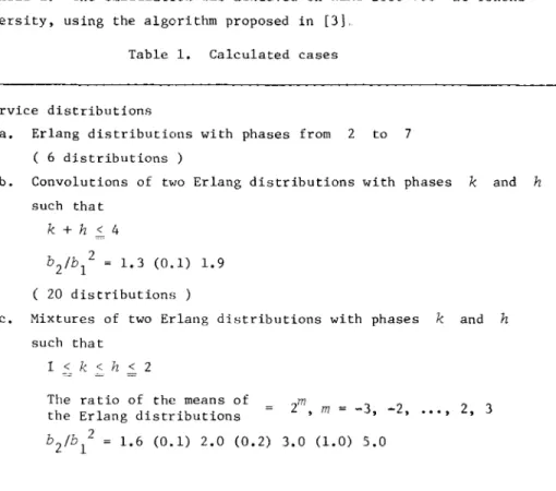
Table 1. Calculated cases

*

Service distributions

a. Erlang distributions with phases from Z to 7 ( 6 distributions )

b. Convolutions of two Erlang distributions with phases k and h

such that k + h < 4

Z

bZ/b₁ = 1.3 (0.1) 1.9 ZO distributions )

c. Mixtures of two Erlang distributions with phases

k

and

h

such that

Zm, m

=

-3, -Z, ••• , 2, 3

The ratio of the means of the Erlang distributions

2

Cl k h

=

1 26 distributions c

2 k 1, h

=

2 67 distributions c

3 k h

=

2 34 distributions

,;'c _{Number of channels c 1, 2, 3 and 4}

*

Traffic intensity p 0.1 (0.1) 0.9

The approximation formulas (1.1), (1.2), (1.3) and (1.5) were tested for queues designated in Table 1. The maximum relati ve errors of the approxima te values are tabulated in Table 2. The result of the test shows the following points:

Comparison between approximations

~(W)

i) Generally, is more accurate than

~(W)

and

~(W)

is more

accurate than

ii) For queues with service distributions in Group a (Erlang distributions) or in Group b (convolutions of Erlang distributions),

~(W)

and EC(W) are satisfactorily accurate.

iii) For queues with service distributions in Group c (mixtures of Erlang distributions), sometimes

~(W)

and

~(W)

are not good, but EC(W) is not so bad.

iv) For queues with service distributions in Group c such that b <

·3 = 2.0 b22/bl i.e., roughly speaking, not long tailed distributions in Group c

~(W)

and

~(W)

are not bad, but _EC(W) is better.

Relative errors of

Ec(W)

and

V c(W)

i) The relative error of EC(W) is within 10% in every case in the test. Also, the relative error of V c(W) is within 21% in every case, and this indicates that t'1e relative error of

~M

which is an approximation of the standard deviation of the waiting time, is within 10% in every case. ii) The result stated above ensures that EC(W) and VC(W) are fairly accurate for queues we ordinarily deal with. However this does not mean that they are always accurate. For a queue with a service distribution with

b =

158

Table 2.

maximum

Y. Takahashi

Maximum relative errors of approximate values

100 x

I

(approximate value) - (exact val~~ (exact value)

The maximization is taken over service distributions in the designated group and over the number of channels c from 1 to 4.

a , band c. (i = 1, 2 , 3 ) ~

in the first column represent groups of service distributions explained in Table I, and c

*

(i = 1,2,3) represent the

i group of service distributions in

Group a b c ₁

*

c ₂

*

c ₃

*

p = .3 = .6 = .9 p = .3 =.6 = .9 p = .3 = .6 = .9 p = .3 = .6 = .9 P = .3 = .6 = .9 P = .3 = .6 = .9 P = .3

=

.6

=

.9 p

=

.3 = .6

=

.9

~~(W)

17.0 7.51 1.46 12.3 5.45 1.06 62.4 30.6 5.33 83.5 39.0 6.52 50.3 25.3 4.47 19.8 8.15 1.50 23.6 9.56 1. 74 7.08 3.71 .77 c. ~ such that b3

~

2.0b2 2_/b 1

~(W)

EC(W) V G(W) .57 .40 1.77 .80 .94 .70 .32 034 .13 2.66 .58 2.45 .73 .83 .55 .23 .29 .11 39.8 5.08 11.1 24.2 7.47 14.5 4.51 1.80 .91 58.0 7.65 19.7 32.3 9.61 20.6 5.70 2.29 2.38 36.4 5.89 14.3 21.2 6.26 12.3 3.93 1.47 1.11 6.27 2.10 7.77 3.97 1.67 2.74 .86 .57 .27 7.85 2.35 5.33 4.26 2.01 2.25 .96 .69 .56 8.24 1. 84 6.85 4.83 1.06 3.21 .94 .32 .81

Appendix.

Some Notes on Calculations of

EC(W)

and

Vc(W)

The values of et,

S,

E,\/W)

,

VM(W)

-

(EM(W) ) 2

,

ED(W) and

VD(W)

-

(E

D(W»2 are tabulated in Tables 3, 4 and 5 below.

I f sample data of the service distribution are available, then one can calculate _EC(Jv) by using Tables 3 and 5 and estimates

1 n 1 n b l

L

and b

L

et X. x. n i=l 1- et n i=l

1-If the service distribution is an Erl.ang distribution with phase

k,

then b et b et 1 1 (k-l)! f (k + et) 1 (1 + a)(l +

%)

ket et (1 + k-l) f (a + 1) • So, using the relation (1.4), one can calculate EC(W) from the formula

1

k~

(1 + a)(l +

i-) ...

(1 +

k~l»

a-I

EM(W)

using Tables 3 and 4. This formula does not contain the ganuna function explicitly.

If the service distribution is a convolution of several Erlang distri-butions or a mixture of such convolutions, then the distribution function of it can be written as where phase such C(x) ~ _{Pi Ek . (x/8 i )} 1-

1-Ek(x) is the distrivution function of the Erlang distribution with k and mean equal to 1 , and p. are (possibly negative) numbers

1-that

_L

p. = 1 Since b = 1 b a

L

i 1-p. 1- 8. 1-8.

1-k.

1.-and )a

--:(::-k~l=---:-l7')-:-!

f(k_i

+

a) i we have

160 Y. Takahashi

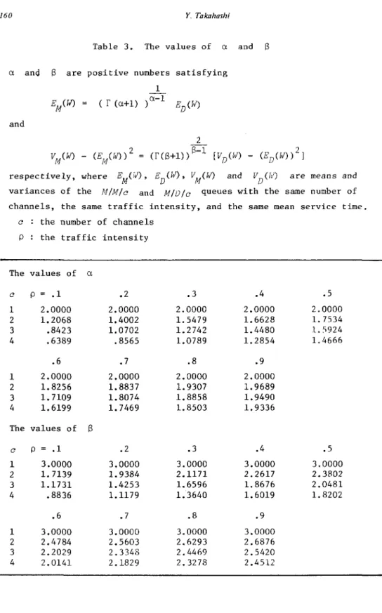
Table 3. The values of a and B

a and

B

are positive numbers satisfying 1

EM(W) = ( f (a+l) )a-1 ED(W)

and

2

VM(W) - CE

MCW»2

=

CfCB+1»B-1 [VDCW) - (EDCW»2]

respectively, where EMer

v) ,

EDCW), VMCW) and VDU';) are means and variances of the M/M/c and M/D/c queues with the same number of channels, the same traffic intensity, and the same mean service time.

c the number of channels P the traffic intensity

The values of a c P = .1 .2 1 2.0000 2.0000 2 1. 2068 1.4002 3 .8423 1.0702 4 .6389 .8565 .6 .7 1 2.0000 2.0000 2 1. 8256 1. 8837 3 1. 7109 1.8074 4 1. 6199 1.7469 The values of 8 c P = .1 .2 1 3.0000 3.0000 2 1. 7139 1. 9384 3 1.1731 1. 4253 4 .8836 1.1179 .6 .7 1 3.0000 3.0000 2 2.4784 2.5603 3 2.2029 2.3348 4 2.0141 2.1829 .3 .4 .5 2.0000 2.0000 2.0000 1. 5479 1.6628 1. 7534 1.2742 1.4480 1. 5924 1.0789 1. 2854 1.4666 .8 .9 2.0000 2.0000 1. 9307 1. 9689 1.8858 1. 9490 1. 8503 1. 9336 .3 .4 .5 3.0000 3.0000 3.0000 2.1171 2.2617 2.3802 1. 6596 1. 8676 2.0481 1.3640 1. 6019 1.8202 .8 .9 3.0000 3.0000 2.6293 2.6876 2.4469 2.5420 2.3278 2.4512

~~(W) is the mean waiting time and VM(W) is the variance of the waiting time of the M/M/c queue.

~ the service rate, i.e., the reciprocal of the mean service time

c : the number of channels

P

the traffic intensity

The values of ~EM(W)

c P = .1 .2 .3 .4 .5 1 .111111 .250000 .428571 .666667 1.00000 2 .0101010 '0416667 · 0989011 .190476 .333333 3 .00 137174 .0102740 • 0333471 '0784314 .157895 4 .000 220677 .00 299401 .0132321 .0377916 .0869565 .6 .7 .8 .9 1 1.50000 2.33333 4.00000 9.00000 2 .562500 .960784 1. 77778 4.26316 3 .295620 .547049 1.07865 2.72354 4 .179402 .357212 .745541 1.96938 The values of ]J2[V M(W) - (EM(W))2] c p = .1 .2 .3 .4 .5 1 .222222 .500000 .857143 1. 33333 2.00000 2 • 0110193 .0486111 . 12172lf .244898 .444444 3 '00101234 '00835053 .02953S0 '0748430 .160665 4 '000122501 . 00185333 · 0 0910129 '0286366 '0718336 .6 .7 .8 .9 1 3.00000 4.66667 8.00000 18.0000 2 .773438 1.35640 2.56790 6.28255 3 .317918 .617139 1. 26853 3.32161 4 .159882 .340152 .752190 2.08998

162 Y. Takllilasili

ED(f/) is the mean waiting time and VDUv') is the variance of the

waiting time of the M/Die queue.

W the service rate, i.e., the reciprocal of the service time c the number of channels

p the traffic intensity

The values of WED(W)

e p

=

.1 .2 .3 .4 .5 1 '0555556 .125000 .214286 .333333 .500000 2 .00 620828 .0242277 .0552594 103311 .176741 3 .000947358 .00658323 .0 200944 .0 450111 .0 872 017 4 .000 164064 .00 205766 .00 845564 .0 226987 .0 496517 .6 .7 .8 .9 1 .750000 1.16667 2.00000 4.50000 2 .293036 .493610 .903284 2.14692 3 .158409 .286247 .553900 1.37791 4 '0983759 .189708 .386095 .999966 The values of ') p-[VD(W) - (ED(W) )2] c p

₌

.1 .2 .3 .4 .5 1 .0370370 .0 833333 .142857 _ 222222 .333333 2 .00 315930 .0 125048 .0 288 624 .0545179 .0941175 3 .000390189 .00 2784 56 .00 87 0264 .0199065 .0392936 4 '0000567977 .000 738733 . 00313982 _00869126 '0195464 .6 .7 .8 .9 1 .500000 .777778 1.33333 3.00000 2 .157322 .266970 .491863 1.17640 3 . 0725915 .133191 .261352 .658550 4 .0397126 .0 7834 96 .162817 .429835

An Approximation Formula for an M/G/c Queue 8. 1

( !

Pi ( 'Z- _)a (l-ta) (1+

I)

(1+ a

»)

_0-1

T.-

...

_k.-l c:'C(W) 'Z- 'Z- EM(W)

(I

Pi 8i)a which can be calculated using Tables 3 and 4.

These notes are also available for calculation of VC(W) with trjvial modifications.

Acknowledgment

An earlier draft of the paper was diseussed in the 5th Management Science Colloquium at Osaka, Japan, in August 1976., The author wishes to thank par-ticipants of the Colloquium and referees for their comments which contributed greatly towards improvements in the exposition.

References

III Lee, A. M., and Longton, P. A.: Queueing process associated with airline passenger check-in. OlleY'aUonal Research Quarterly, Vol. 10 (1957),

pp. 56-71.

121

Page, E.: Queurdnu Th(?oY'!! 1:n OR, Butterworth, London (1972).

IJ1

Takahashi, Y., <lnd Takami, Y.: A numerical method for the steady-state probabilities of a GI/G/c queueing system in a general class •

• 1. Opcmtions Resear'ch Society of Japan, Vol. 19 (1976), pp. 147-157.

Yukio TAKAHASHI: Department of Business Management, Faculty of Economics Tohoku University, Kawauchi, Sendai, 980, Japan