A Production Planning Model for Multi-Product Facilities

Society of Japan

Vol. 28, No. 4, December 1985

Abstract

A PRODUCTION PLANNING MODEL FOR

MULTI-PRODUCT FACILITIES

Chang Sup Sung

Korea Advanced Institute of Science & Technology

(Received April 5, 1985: Final September 18, 1985)

A production planning model for multi-product facilities is analyzed, in which known demands must be satisfied. In the model, in every production period each facility produces a certain number of items each taking a fixed part of the production amount. Concave production costs dependent upon the production in different facilities and piecewise concave inventory costs are considered. Both the nonbacklog and backlog permitted cases are considered. The structure of an optimal solution is characterized and then used illustratively in a simple dynamic programming algorithm for nonbacklog single-facility problems.

1.

Introduction

Wager and Whitin [2] have analyzed an important product, single-facility production and inventory problenl. Assuming that demands for the product were known, they sought to find a production schedule, in terms of how much to produce in each period for the n~'xt N periods, that minimized the cost of producing and holding inventory. They further assumed that the production and inventory cost functions were concav~' and that no backlogging of unsat is-fied demand was permitted.

Florian and Klein [1] have considered the problem of Wagner and Whitin [2] under the assumption that the production levels are restricted to the period-dependent capacity limits. They have also considered the backlogging case in the work, while a dynamic programming algorithm was suggested only for the problems with a fixed capacity limit.

Zangwill [3] has considered a multi-·product, multi-facility model, which is, however, a 1 inking together of the single-product single-faci 1 ity model. He has also studied a multi-echelon model only for a single product in another paper [4].

346

cs.

Sung

In this paper, three different cases of production planning for multi-product facilities will be analyzed, The first two cases are for the problem of multi-product single-facility production planning with and without backlog, respectively, and the last one is for multi-product multi-facility production planning problems with backlog that is essentially a linking together of the backlogged single-facility cases and so forms an acyclic network of the facili-ties. In each case, in every production period each facility produces multiple items each taking a fixed part of the whole production amount. As an example, an oil refinery problem can be taken into account, where some amount of crude oil may be refined to produce two different items, gasoline and some fine chemical resources, in the fixed production amount ratios, say a

1>O and a2>O percentages, respectively. Concave production costs dependent upon the pro-duction in different facilities and piecewise concave inventory costs are considered.

The objective of this paper is to find a useful description of the struc-ture of optimal plans for each case. They consist of independent subplans ~n which in each production period except the last, where all the demands are exactly satisfied, at least one of the demands for different items is exactly satisfied. Each feasible plan consisting only of such subplans is proven to be an extreme point of the feasible production schedules set for the single-facility problems and also to be an element of the dominant set (defined by Zangwill [3]) for the multi-facility problem. This characterization is then illustrated by a simple dynamic programming algorithm for the nonbacklogged single-facility problem.

2. Single-Facility Case with Nonbacklog

2.1 Model formulation

Consider a M-product problem with each product i (item i)(i=1,2, ... ,M) taking ai>O parts of the total production amount in every period. That is, the amount produced in each period (x

1,x2, ... ,xN)=X has the relations M

(1) x

t L

Xu

and xti xt

.

(ai/Ma)

,

i=l

M

where M _{La" and x ti is}

a _{j=l J} the production amount of item i in period

t(t=1,2, ... ,N; i=1,2, ... ,M), Let T

1, ... ,TN represent the known demands over

the planning horizon N, where T

rt=(rt1,_ .. ,rtM)' The component rti?:O represents the demand for item i in period t. Note that each demand r

ti is not necessarily required to take ai parts of the total demand in period t.

There is no loss in generality In assuming that both the initial inventory and the final inventory are zeros. Its reason is that if the equality of

M m

"R

1 N (i)/ j=1

I

R1 N (j) = a ~ ./M " a (where R£ _m

(i)

=

t=£

I

rt ~ ,) does not hold for any i,

some additional (artificial) demands can be considered to adjust each of the last demands to the equality. Then, the problem is to minimize the total costs of production and inventory, say

G (x)

subject to

Iti X 1t (i) - R

1t(i), ¥i and t M x t

I

Xti ' ¥t i=1 (p 1) x

ti (a/a1) xt1 ' "fi and t Iti ~ 0 and x_ti ~ 0, "fi and t

o

m

where x£m(i) =

I

Xt" (£=1, ... ,N-1; m=£, £+l, •.. ,N), and et is the concave

t=£ ~

production cost function for period t, and Hti gives the concave cost of storing the inventory quantity Iti of item i from period t to period t+1.

The constraints of the problem (P

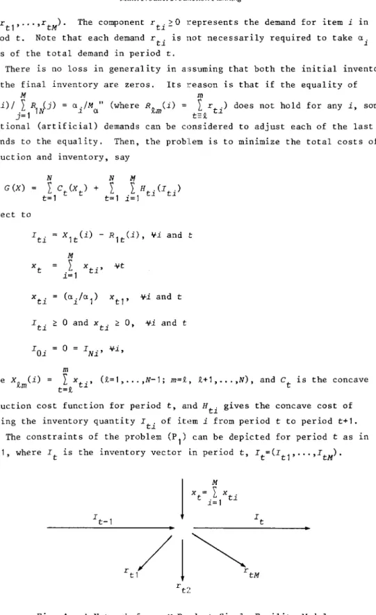
1) can be depicted for period t as In Fig.1, where It is the inventory vector Ln period t, It=(Itl, ... ,ItM)'

M

x =

I

x t i=1 ti

348 C. S.Sung

The constraints of the problem (PI) define a closed bounded convex set. Since G is concave, we know that it attains its minimum at an extreme point of the

set. Let D be the set of all the extreme points of the feasible solutions set. The characterization of D will then be made in the next section, which will be used to facilitate finding an optimal production plan.

Consider the following inventory decomposition property (see Florian and Klein [1]) for its proof) upon which our approach is based.

Theorem 1.

(Inventory Decomposition Property). Suppose that the con-straints, I~i=O for all i and some ~E

{l,Z, ...

,N-l}, are added to those de-scribed in the problem (P

1). Then, an optimal solution to the original problem can be found by independently finding solutions to the problems for the first ~ periods and for the last N-~ periods.

2.2 Characterization of extreme point

Let us introduce an "at-Ieast-one exact requirement sequence" that will form the basis for our characterization of D.

Definition.

A production sequence (xl ,x

Z, ••• ,xN) is called an "at-least-one exact requirement sequence" if for every n (l~n<N) such that xn+l > 0,

n

I

x =L(n), where L(n)=max{(M /a.)R

1 (i)}.

t=1 t i a ~ n

Note that L(n) is equal to the lower bound of cumulative production amount from period 1 to period n. Each feasible plan forming an at-least-one exact requirement sequence is then characterized as the correspondence to an element of D.

Theorem 2.

A feasible plan X is an "at-Ieast-one exact requirement se-quence" Hf it is in D.

Proof:

Suppose X E D, and X does not form an at-least-one exact require-ment sequence. Hence, there is at least one production period, say b, l::;'b<N,

in which for every i E {1,Z, ... ,M},

and further, among them at least one item j is in "partial" inventory, i.e.,

o

< I

b- 1,j < Tbj, where o(b) is the last production period prior to period b.

Without loss of generality, we suppose that there is just one such period. Let

where J is the set of partial inventory items,

J

is the complement of J and

(a1/aj)Ib_l,j is the inventory amount of item j computed in terms of item 1, and let Ut be a N component vector with a unity element in the tth position. and zeros elseqhere.

Now, define the distinct production plans X'

=

X - CUa(b) + cUb and

X"

Since 0 > 0, these plans are easily seen to be feasible. However. X

=

1/2 (X' + X"), contradicting our assumption that X is an extreme point. This proves "if part".

Suppose on the contrary that xrjD. Then, there are feasible distinct plans X' and X" such that X (X' +x") • This implies, however, that by hypo-thesis there exists an item j E: {1.2, .•• ,M} such that in a production period

b(lSb~N), (a/M_a)L(b-1)=R₁,b_l(j) and so either I1r-l,j<O or I~_l,j<O, where I~_l,j and I

b-1, j represent the inventory levels of item j, at the end of

period b-l, associated with the two plans

x'

and

x",

respectively. This contradicts the assumption that both

x'

and

x"

are feasible.

Thus. the proof is completed.

Theorem 2 implies that the set of all at-least-one exact requirement sequences is D. Therefore, one of such sequences having the minimum cost becomes and optimal solution.

2.3. An Algorithm

Before developing our algorithm it 1S necessary to specify how to deter-mine each component x

t* (t=O,l, .•. ,N) of an optimal solution x* in somewhat

more detail.

The descriptions of the elements of D given in Theorem 2 can be used to facilitate finding an optimal plan X*. I t follows from Theorem 2 that all extreme point solutions, including the optimal one, have the property that

M

IT I .X =0 (t=1,2, ... ,N). This leads to Corollary 1.

i=l t-l,~ t

Corollary 1.

An optimal production plan x* consists of component x~'s

M

such that IT I .x*=O for t=1,2, ... ,N. i=l t-1,~ t

Denote by xm+1(n) the amount of the production completed in period m+l, OSm<n~N, to satisfy the demands over the periods from m+l through n, where for

350 C. S.Sung

.M .M

all i,I

ti>

°

(m<t<N), _i=l IT.I _nu .=0 and IT I .=0. _{i=l n~} Then, each optimal quantity

x~l(n) can be determined immediately based on Corollary 1.

the results of Theorem 1 and

Theorem 3.

An optimal production plan X* consists only of component

X*'s (m=0,1, ... ,N-1) satisfying the relation

m

X~l(n)

=

L(n)-L(m) for OSm<nSN.

The results of Theorem 3 indicate that an optimally production plan can be found by searching optimality for (m,n) sequences. Thereupon, a dynamic programming recurSl0n shall be exploited.

Let d denote the production and inventory costs associated with pro-Ill1l

ducing the amount of xm+l(n). Then, dIll1l can be expressed as follows:

(2) d

Ill1l

n .M

= cm+1 (xmt1 (n» +

I

I

_{HtJ·(I tJ·),}

t=m+1 j=l

where Itj(m+lstsn) are the inventory levels associated with production xm+l(n)

in period m+l.

The results of Theorem 3 and d values can be applied to form a dynamic Ill1l

programming recursion using the periods 0,1,2, ... ,N as states. Let Ft be the cost associated with an optimal production plan over periods 0,1,2, •..• t

.M

(t=O,l, ... ,N), given that IT It.=O. i=l ~ Then, (3) F n and F_O == 0. min O~m::;;n-l [F + d ], m Ill1l (n=1,2, •.. ,N)

The recursion (3) indicates that the minimum cost for the first n periods comprises the setup and production costs in period m+l, the charges for filling demand r

t(t=m+l, ... ,n) by carrying inventory from period m+l, and the eost of

adapting an optimal policy in periods

°

through m taken by themselves. Theo-rems 2 and 3 guarantee that at period n we shall find an optimum plan (sche-dule) of this type.

Now, the results of Theorem 3 and the relations (2) and (3) are put together to give the following step-by-step description of the solution pro-cedure:

Step 1 (Initialization): Set FO=O, n=l, and .m=O. Step 2: Compute d

mn values for each m (OSm:::n-1) by use of Theorem 3 and

Step 3: Apply the recursion (3) for finding each optimal policy Fn' and

repeat Steps 2 and 3 with In=n+1" until the last period " n=N".

The algorithm described above indicates that to determine an optimal policy Fn in period n by use of the recursion (3), in general, n(n+1)/2

com-putations for the values of dmn's (O~m$N-l) are required. Therefore, finding an optimal plan x* is, in general, a tedious combinatorial problem when N is large.

2.4. An example

We illustrate the algorithm with the 6 period two-product single-facility problem and with the production ratio of "et

1:et2

=

2:3". The production and

inventory cost functions are given as follows:

Ht1 (It 1 ) 3t It1 ' and

H t2(It2) = 2t It2, where O(x t) = { 0, i f xt 0

,

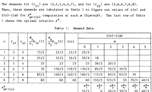
t=1,2, ••• ,6. 1, i f x t > 0 The demands for {r

t1} are (3,2,5,4,3,7), and for {rt2} are (5,6,4,7,6,8). Then, these demands are tabulated in Table 1 to figure out values of L(n) and

L(n)-L(m) for X~l (n) computation at each m (O:::m<n:::N). The last row of Table 1 shows the optimal solution

X*.

Table 1. Demand Data

M M L(n)-L(m) n _{rnl rn2 ""::R} 1 (1) ""::R 1 (2) L(n) m et 1 n et2 n 0 1 2 3 4 5 1 3 5 15/2 25/3 25/3 25/3 2 2 6 25/2 55/3 55/3 55/3 10 3 5 4 25 25 25 25 50/3 20/3 4 4 7 35 110/3 110/3 110/3 85/3 55/3 35/3 5 3 6 85/2 140/3 140/3 140/3 115/3 85/3 65/3 10 6 7 8 60 60 60 60 155/3 125/3 35 70/3 40/3

x*

_{m+ 1 (n)} x*= 1 x*= 2 x*= 3 x*= 4 x*= 5 x*= 6 55/3 0 20/3 35/3 10 40/3

352 C.S. Sung

The solution procedure in section 2.3 is then applied to the example, and

F

1, F2, F3, F4, FS and F6 are calculated as follows: F1=FO+d01=0+343/3=343/3

with x~(1)=2S/3; F₂=min{F_{O+d02 '} Fl+d12}=FO+d02=7S7/3 with x~(2)=SS/3; F3=

0~2{Fm+dm3}=F2+d23=1017/3 with x~(3)=20/3; F4=0~~3{Fm+dm4}=F3+d34=1436/3 with xZ(4)=3S/3; FS= min {F +d_mS}=F₄+d_4S=1841/3 with X~(S)=10; F6= min {F +d_m6}

0;;; m;; 4 m

o;;;m;;s

m

=F

S+dS6=22S6/3 with x~(6)=·40/3. Thus, the optimal solution of the problem is

X*=(SS/3, 0, 20/3, 3S/3, 10, 40/3).

3. Single-Facility Case with Backlog

The model described in section 1 may be extended so that backlogging is permitted. We shall assume as in Zangwill [4] that all demands must be satis-fied no longer than S. (j=1,2, ••• ,M) periods after the specified delivery data

J

for each item j. Thus the constraints Itj ~ 0 in the problem (Pl) is replaced by

rh" for all j and t, 1J

t=S .,8 .+l, ••• ,N.

J J With backlogging, we assume that for each item j a penalty

cost is charged on the amount backlogged in any period and the cost is concave, so that the total inventory cost is piecewise concave.

Although the objective function of (Pl) is then piecewise concave rather than concave, all of the results obtained for the nonbacklog case hold. Since the arguments are, with slight modifications, the same as for the nonbacklog problem, we shall not repe!at them in detail. However, we shall indicate note-worthy changes in this section.

The property of Theorem 1 still holds in the case where the backlogging constraints are additionally considered in the problem (Pl), so that the re-cursion (3) may still be used.

Theorem 4.

Suppose that the constraints, I£i=O for all i and some

t

£dl,2, ... ,N-l}, are added to those described in (p1) and if I >-

I

r.,

t r h=t-S.+ 1 hJ J

t=£+l, £+2, ... , N, where r

hj

=

°

for h $ 0, then an optimal solution to the

extended problem can be found by independently solving the problems for the first £ periods and for the last (N-n periods.

Following Zangwill [4], the set of all feasible solutions can be parti-tioned into disjoint subsets, called "basic sets", which are characterized by whether the quantity Itj is nonpositive or positive for each item j in each

period t, t=l ,2, ... ,N-1. Letting fl be the set of all feasible solutions that satisfy the constraints of the extended problem, then fl is the union of

all 2M(N-1) basic sets. Each such subset is closed, bounded and convex with

a finite number of extreme points and further, the objective function, G (x), is concave on each given basic set. Thus for a fixed basic set, G(x) attains its minimum at one of its extreme points. Thereupon, letting D be the union of all extreme points of all basic sets, then the minimum of G (x) occurs at a point in D.

The above properties lead to our conclusion that the characterization of

D for the extended problem can be given similiarly as in Theorem 2 with the newly defined "at-least-one boundary sequence".

Definition.

A production sequence (xl ,x

2' ••• ,xN) is called an

"at-Ieast-one boundary sequence" if for every n (l:::n<N) such that xn+l > 0,

n

I

xtE{L(n), Ls(n)},

t=l

where La(n) = max{(M /0..)R

1 a (i)}.

~ i 0. ~ ,n-~i

Then, each feasible plan forming an at-Ieast-one boundary sequence is characterized as the correspondence to an element of D for the extended problem. This shall now be proved.

Theorem 5.

A feasible plan X is an "at-Ieast-one boundary sequence" iff it is in D.

Proof:

The proof of "it part" can be completed easily by following the proof steps of Theorem 2 with the newly defined 0 ' ;

0 ' =

fmin[~in+{(o./o.

.)I_b- ₁

J,

min_{-(o.l/o. .)I_b-₁ .,

J£J ] ,] jEJ ] ,J

b-1

(o./o.J') _{(Ib - 1},J' +

I

_{r R .)}],}

R.=b-S. ,J J

where J+ and ,7 represent the set of items having on-hand and backlogged inventories, respectively.

For "only if part", suppose on the contrary that Xf/D. Then, there are 1

feasible distinct plans x' and x" such that

x-2(x ' +x").

By hypothesis, there exists an item je{1,2, ••• ,M} such that in a produc-tion period b (l<b<N), either (o../M )L(b-1)=R

1 b 1(j) or (o../M )L(b-1)=

- - Jo. , - Jo.

R1 ,b-S ,-1 (j). Thereby, either x' or x" is infeasible, or x' and x" belong to

differ~nt

basic sets, which contradicts the assumption that both x' and x"

are feasible.

354 C.S. Sung

Now, it will be discussed about how to determine x~l(n) required in each

d computation for the extended problem. In fact, a similar procedure to mn

that in section 2.3 can be constructed, since in view of Theorem 5 an optimal solution should form an at-Ieast-one boundary sequence.

Theorem 6.

For the extended problem, an optimal plan X* consists only of component x;'s (rnrO,l, ... ,N-l) satisfying the relation x:+₁(n)=(L(n)-L(m» or (LS(n)-L(m» for OSm<nSN.

The results of Theorem 6 indicate that the solution procedure given in section 2.3 can be directly applied to the extended problem with the options for each x;+ l(n) value. Therefore, it seems rather more difficult to search all the associated extreme points.

4. Multi-Facility Case with Backlog

4.1.

M

products at each facility

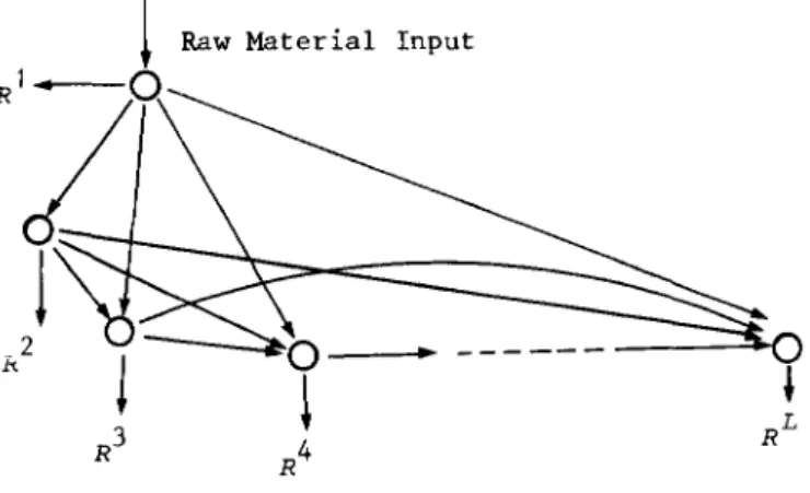
The model described in section 3 may be extended to the multi-facility problem treated in Zangwill [3], where L individual facilities are linked together to form an acyclic network depicted in Fig.2.

.2 ~

Raw Material Input

Fig. 2. The Acyclic Network with L Facilities.

In the model, each facility except the first facility is allowed to re-ceive inputs from raw materials or lower numbered facilities (not from itself or higher numbered facilities), then in each period manufacture M specific products on its own production line. Each product is then stored in inventory until needed either to satisfy demands for each product or to supply inputs to other faciliteies.

b b b b b

R = (r

1, r2, ••• , rN), ri;::O, represents the market requirements vector

b

for facility b (b=l, ••• ,L) over the planning horizon N. Further, each r_t itself is a demand vector composed of M different demands, i.e., rb

=

{~t

,},

t ]

where

r~j

represents the demand for item (product) j (j=1 ,2, ..• ,M) at facility

b in period t,

l~t~N.

Assuming that all demands

r~j

are fixed and known, we shall seek to determine the general form of the minimum cost production sche-dule (plan) that will specify how much each facility in the network should produce.

b P

Let x

t ::: 0 be the production completed in period t at facility band _b I t ' _] Let a? _] >

_-

°

be the inventory of item j at the end of period t in facility b.

the number of units of facility b's product j required to produce one unit of facility g's product j. It'is assumed that facility b can have a time lag Ab in production and thereby production started in period t is completed in period

t+A

b• Then, the amount of item j desired out of facility b in period t as

~

bg g

inputs to other facilities is L a

j xt+A " and the total demand on

facil-g=b+1 g'] b

ity b in period t and the inventory level, denoted respectively by Y_{t j} and

~j'

are b

~

bg g r_{t ],} + L a , x_t+_A g=b+1 ] g and b t b b

Itj

=

L

(xhj-Y_hj) for all t, j and b. h=l

It ~s also assumed that each facility can backlog total demand for its product a certain fixed integral number of periods. Let B, b represent the

]

number of periods of backlog permitted for t

item j at facility b. Then, the

b

backlog limit for each item j is Itj

::: - L

_b h=t-B ,+1

]

Further, assume that

~j

=

0 10 ' b for all band j.

J

1 2 2 I. L

(X₁' · · · ' X_{N '} X₁'···,X_{N ' · .. ,} x₁" " ' x ) denote

b N b b

for the entire network, where X = (xl"" ,x N) 1

x2, xL)

Let

z

= (X , ...

,

=

the production schedule (vector)

represents the production schedule for facility b and each

x~

is

decomposE~d

b b b b b b b

into M different products, X

t j' such that Xt' «(J.j/M~) = Xt j with (J.j(or M~)

representing the fixed production ratio of item j at facility b. Let zb =

(xb , b+1 X , ...

,x

L) be def~ne ' d as a part~al product~on - - sche u e d 1 ~n fac~ ~tH'S - '1" b

through L. Let

~ = (Y~' y~,

•••

'Y~)

represent the total demand for facility b.

b+1 b b b+1

z completely specifies Y-, so that it is convenient to write r (z ) to

b b+1

356 C. S.Sung

zg is said to be feasible if the above constraints hold for all b~g and all t.

~f g+ 1 . f . I g g+ 1 . g

Similarly, L Z ~s eaS1b e, X is said to feasibly supply Z ~f z

=

(xg, zg+l) is feasible.

Although each facility in the network produces M different items in each period, all the results obtained for the single-facility case hold, since the arguments at each facility are the same as for the problem in section 3. We shall not repeat them all here in detail. However, Lemma 1 shall be proved to make the confirmation of the results easy.

Let D be the dominant set, which is the union of the extreme points of all the sLMN basic sets, and Db denote the partial dominant set constructed from facilities b through L.

b+l -b+l -b+l .

Lenma

1.

Let Z , Z , Z be feas~ble partial production vectors such that zb+l '" zb+l, and zb+l

=

f(Zb+l+ z b+l), b~l. Assume xb feasibly sup-plies zb+l and that it forms an at-least-one boundary sequence for

~(zb+l).

Then, there exist production vectors X and X that feasibly supply Z -b -b -b+l and

b b+l 1 -b -b+l -b -b+l

respectively, such that (X , z )

=

2[(X-'

z ) +

(X-,

Z )].

zb+l

_,

b -b b -b

Furthermore,

It

~

°

iff It ~ 0, and

It

~ 0, iff It ~

°

for all t, t=l, ... ,N.

P

roo:

f From t e h ~nventory constra~nts . . an d the re I ' at~on, Z b+ 1 ( .) J =,

1 -b+l . -b+l, b+l, , ,

2(z (J)+z (J» (Z (7) denotmg the part~al production vector for item

j), there exist real values, 0tj' such that

b b b+l

Since X forms an at-least-one boundary sequence for y-(z ), there are integers

°

such that

s(O,j) ~ s(l,j) ~ ••• ~ S(N,j)

=

N for each item j £ {1,2, •.. ,M}

s(t,j) b

L

Y_hj

h=s(t-l,j)+l

Define, for each item j,

-b s(t,j) b X t j _h=s(t-l,j)+l

L

(Yh ,-0 h ) and J -b s(t,j) b X tj

L

(Yh,-O hj) h=s(t-l,j)+l J

Then, the proof can be completed just by following the proof steps of Lemma 1 in Zangwill [3].

Theorem 1 in Zangwill [3], Theorem 7 (which characterizes the structure of the optimal solution) can then be easily proved.

Theorem 7.

A feasible plan z

=

(X'I,

x

2, ••• ,XL) consists only of each facility's at-Ieast-one boundary sequenc:e for each zb+1 in Db+1 for all b iff it is in D.

4.2. Higher-numbered products at each facility

Consider again the acyclic network problem with each facility allowed only to manufacture the higher-numbered but different items in each production period. That is, in each production period, facility L produces a single item, facility L-1 manufactures two different items (one for its own market require-ments and the other one for inputs to facility L), and so on. In fact, L

=

M.

Facility 1 is then required to manufacture M different items in each production period to satisfy its own demands and supply inputs to other facilities.

All of the results obtained for the problem in section 4.1 still hold. However, in comparison with that in section 4.1, this problem is rather simpler in determining an optimal production veetor, since it has, in general, the

. NM(M+1) /2 .

much smaller number of bas1c sets, 2 , and each of the extreme p01nts at each facility can be directly searched by applying Theorem 5 in section 3 with each adjusted number of items.

5. Concl usion

In this paper, we have found a useful description of the structure of optimal plans which form at-Ieast-one exact (boundary) requirement sequences. The optimal plan structures have also been shown to hold for the nonbacklog models on both single-facility and multi-facility systems. This solution characterization has then been incorporated in constructing a dynamic pro-gramming algorithm. The algorithm may be practically and efficiently used to find optimal solutions for small-sized problems.

It is further noticed that as an hmnediate extension, a capacitated multi-product model can also be handled in the framework of this paper.

Acknowledgement

The author wishes to thank the referees for their numerous valuable comments and suggestions.

358

References

[1] Florian, M. and Klein, M.: Deterministic Production Planning with Concave Costs and Capacity Constraints. Managemant Science, 18 (1971), 12-20. [2] Wagner, H. A. and Whitin, T. M.: Dynamic Version of the Economic Lot Size

Model. Management Science, 5 (1959), 89-96.

[3] Zangwill, W. I.: A Deterministic Multi-Product, Multi-Facility Production and Inventory Model. Operations Research, 14 (1966), 486-507.

[4] Zangwill, W. 1.: A Backlogging Model and a Multi-Echelon Model of a.

Dynamic Economic Lot Size Production System - A Network Approach. Manage-mant Science, 15 (1969), 506-527.

C. S. SUNG: Industrial Engineering Department, Korea Advanced Inst.itute of Science & Technology,

P. O. Box 150, Cheongryang Seoul, Korea