(r, Q) Policy for a Single-Product Production/Inventory Problem with a Compound Poisson Demand Process

(1)

Journal of the Operations Research Society of Japan

Vo!. 30, No. 2, June 1987

Abstract

(r,

Q)

POLICY FOR A SINGLE-PRODUCT

PRODUCTION/INVENTORY PROBLEM WITH

A

COMPOUND POISSON DEMAND PROCESS

Chang Sup Sung Geun Tae Oh

Korea Advanced Institute of Science and Technology

(Received July 25,1985; Revised August 18, 1986)

This paper considers an optimal (r, Q) policy for a single-product single-machine production/inventory problem with a compound Poisson demand process and backloggings allowed. Under the assumption that during each production period the cumulative amount of production is greater than that of demands in expected term, the associated inventory process is found to be an ergodic Markov chain with infinite states. Thereupon, the steady-state probability distribution is derived. Further, the total cost in the production/inventory system is expressed in terms of the long-run expected average cost, C(r, Q), which is verified as the convex function of r, given Q fixed. A solution proced~re is illustrated with a numerIcal example having random demand sizes taking values one or two.

1. Introduction

This study considers a single-product single-machine production/inventory control problem over infinite time horizon. For the problem, demands for the product are assumed to follow a stationary compound Poisson process with the mean occurrence rate A. It is also assumed that unsatisfied demands are

back-logged, that the machine has a mean production rate ~ such that during each production period the expected cumulative amount of demands is less than that of production, and that the unit production (processing) times are independent and identically distributed, and further independent of the demand process. Moreover, each product unit will be individually stored in inventory so that the production/inventory system will have continuous inventory replenishments with these individual stockings during each replenishing interval (production interval). This replenishment mechanism makes the problem different from the ordinary warehouse-type inventory problems for which replenishments are made

132

(2)

Production/Inventory Problem 133

in batch (lot-size).

Three cost components in the system 1Nill be considered: production cost, inventory holding cost and backlogging cost. Each production will incur a fixed setup cost and a direct production cost charged at a function of]J. The unit-time charge rates for both inventory holdings and backloggings are also assumed to be constant.

Many authors ([2],[4],[5],[8],[10], and [15]) have considered the above problem under the assumption of a Poisson demand process, while Graves and Keilson [6] have treated a problem with a compound Poisson demand process having an exponential demand size distribution. They all have analyzed the problem under the (r,R) production/inventory policy for which whenever the inventory level falls below r, the system needs be operated for production until the inventory level reaches R.

Under the (r,R) policy, production time intervals from the beginning of each production till reaching the inventory level of R are strongly dependent upon demand processes. For a compound Poisson demand process, as assumed for this study, some of such production intervals may get large due to the possi-bility of huge demand occurrences. This implies that the (r,R) policy may not be realistic for production systems with facilities (machines) whose opera-tions are constrained with a regular maintenance work scheduled after each specified length of continuous operation time. For example, some production facilities may have the physical restriction that after each three-day-Iong consecutive operation one day needs be reserved for maintenance.

The above discussions indicate that for problems with such physical restrictions, the (r,Q) policy may appear more realistic than the (r,R)

policy, since the former presumes that each production operation is terminated after producing the fixed amount of Q. Moreover, no one has treated the (r,Q) model yet. The objective of this work is thus to find an optimal (r,Q) policy for the single-product single-machine production/inventory system with each operation physically restricted by a fixed length of consecutive operation time per setup (i.e. by the production quantity, Q, per setup).

The proposed problem is often encountered for production planning manage-ment Ln a variety of manufacturing areas. For example, some companies in machinery industry may have a production system with operational restrictions subject to capacity limit (e.g. restriction by a facility's production capa-city in automobile manufacturing company) whenever an operation is set up. In such cases, Q itself can be a design parameter for the associated capacity determination or an operational decision parameter for an optimal production scheduling. Similarly, some computer terminal operation scheduling can be

(3)

134

c.

S. Sung & G. T. Oh

accounted as in the problem category when each terminal operation needs be regulated during a specific hour each day for the better time-sharing purpose.

2. Steady-State Probability Distribution of Inventory Process

The following notations are considered for formulating an (r,Q) produc-tion/inventory model: for nonnegative integer set Nand nonnegative real value set R+, F (t) F (t) n F* (s ,n) 1

III

D(t,t+u]

distribution function of production time per unit, t £ R+, n-fold convolution of F(t) with itself, where FO(t)

=

1, and F₁(t)

=

F(t), t £ R+,

Laplace-Stieltjes transform of Fn(t)(= [F*(s,l)]n), t £ R+, Re(s)'?O,

mean production time per unit,

cumulative demands during (t,t+u] , where D(u) D(O,U] , u,t £ R+,

mean demand arrival rate,

discrete random demand size with E[~]<=,

probability of demand j representing p{~

L

p .zj,

I

z

I

~

1 ,

j=O ]

j } , j £ N ,

K fixed setup cost,

C(ll) production cost per unit depending on the production rate ll,

h constant holding cost per unit time,

b constant back logging cost per unit time.

A compound Poisson demand process with parameter

A

gives the probability of cumulative demand k in a time interval (O,t],

k

(1) P{D(t) = k} = }: n=O

where qn(k) is the n-fold convolution of the demand size distribution at k with qO(k)=O for k?l, q (0)=0 for n~l, qO(O)=l, and q1(k)=P

k for k?l. Let

k n

ljJ (0)

=

1 and ljJ (k)

e [(At) /n!]q (k)F (t)dt o n=O n m k n " 1 ( ")

- L [L

[(-A)~- /i!]F* ~ (A,m)]q (k),

n

n=O i=O and

(5) B (2)

L

F*(A-AP(Z), Q), for Izl~1. n=O

Now we will show how the (r,Q) production/inventory model can be

described in view of the Markov renewal theory. Let X(t) denote the inventory level at time point t with state space S = {Q+r,Q+r-l, ... ,r, ... }, and let Tn' n?l, be the n-th setup (or shutdown) time point of production operations. That is, each T , for n~ 1, can be interpreted as either the setup time point,

n

if X(T_n_₁) = i for i>r, or shutdown time point, if X(T_n_

1) = i for i~r. Let y(t) represent r+Q-x(t) for a time point t. The resulting process {y(t) t £ R+} will then be called the "inventory process" with state space S* =

{O,I,2, ... }. Denote by Yn' n~l, the state of the inventory process at time point Tn with YO

=

Y(O). Note that each Tn' for n?l, can be interpreted as either the setup time point, if Y 1 = i Eor i<Q, or shutdown time point, if

n-Y_n-₁

=

i for i?Q. We will assume throughout this work that Q~I, and r+Q?O. Since the discrete compound Poisson demand process is memoryless, the transition from a state Y

n = i to Yn+1 = j is Markovian, and the distribution

of the time interval, T_n+₁-T_ndepends only on Y_n. This property leads to Proposition 1 (Cinlar [3]).

Proposition

1.

{Y , T

n n n £ N} is a Markov renewal process, and {Y(t) t £ R+} is a semi-regenerative process.

Denote by G j (t) the probab ility that the time interval, T n+l-T n' is less than or equal to t, given a state j of the process {y ; n £ N}. Then, for

n

(5)

136 (6) G . (t) ]

c.

S. Sung & G. T. Oh l-P{D(t)~Q-j-l}, for OSj<Q, for jS{}. Also denote by P

i j the transitior, probability from the state Yn j: that is,

(7) P

i j = p{Yn+1 = j

I

Yn =

n,

for i , j £ S*.

i to Y n+1

Then, the associated transition probabilities of the process {y ; n £ N} can

n

be characterized as follows:

(i) for either i<Q and j<Q, or i?j+Q+l with j?O,

(8) P, , = 0;

~J

(ii) for i<Q~j, letting s£ be the size of £-th demand and ~ be the total number of demand occurrences during (T ,T 1]

~(j-i-m)pm; m=j-Q+l

(iii) for Q~i~j+Q,

P, ,

~J P{D(T ,T n n+ 1]

=

j-i+Q

I

Y n

i}

~OOp{D(t)

=

j-i+Q}dFQ(t)

a. '+Q(Q) , which leads to the relation that

J-~

=p ,form?l.

i+m,j+m

Letting M = {Pij} be the transition matrix associated with the imbedded Markov chain {y ; n £ N}, it is then characterized as in Theorem 1.

n

Theorem 1.

The chain M is ergodic.

Proof:

With reference to Neuts [9], the next three conditions are suffi-cient for the result.

Condition 1: For Q~l, g.c.d. (Q, d) = 1, aO(Q»O, and

aO(Q)+ ... +a

Q(Q)<l, where d = g.c.d.{k ; ak(Q»O, k?l}.

(6)

Production/lnvlmtory Problem

Condition 2: The matrix I-MO is nonsingular, where the matrix MO is defined by

PQ-1 ,0 PQ- 1 ,Q-1

CP

Condition 3: a*<Q, where a*

=

I

kak(Q). k=O

137

In fact, all Pij'S in (10) are positive from the assumption on the demand process and the production time distribution, so that Condition 1 is satisfied.

From (8), MO is constructed as a null matrix, so that I-MO is a non-singular matrix. Thus, Condition Z is satisfied. Furthermore, since ak(Q) P {D(T -T) = k}, a* = AQE [1',;] Ill, the assumptions on the mean production

n+1 n

rate and the mean demand rate lead to the relation, AQE[I',;]I\l<Q. Therefore, Condition 3 is satisfied. This completes the proof.

Let TI

=

(TI

O' TI1, TIZ' ... ) be the steady-state probability distribution of {y . n £ N} and let

n '

(11) ~jk(t)

=

p{y(t)

=

k

I

YO

=

j}, for j,k £ S*.

Then, the limit of ~jk(t) can be given from Theorem (10.6.12) of Cinlar [3] as follows:

( 1Z) _~k lim ~jk(t)

r

tdG . (t) Q-f 1 1jJ(k) lA, for O:s.j<Q,

(13) m. { o ] k=O

]

r

tdFQ(t) QIll j?Q

Thence,

(i) for O~j<Q,

k-j+n-l}[F n_1(t) - Fn(t)], n=j-k+l for k>j-Q.

These characterizations of Ljk(t) lead to the following detailed expres-sions of

<P

k

Joo[

I

1I.L 'k(t)]dt/L'I o j=k ] ]

TjJ(k)/A-Q/]l] + Q/]l.

j=O ] ] j=O ] k=O

3. Long-Run Expected Average Cost

We can see that

<Pk

is a function of Q but not of r. Therefore, denote by C ,(t;r,Q) the expected system cost incurred during a time interval (O,t]

asso-]

ciated with the (r,Q) production/inventory policy, given Y

(8)

Production/Inventory Problem 139 from the assumptions on the associated cost structures, the system cost C . (t jr ,Q) can be represented by summation of

J 0

cost,

c.

(tjr,Q), the expected holding cost,

the expected setup and production 1

C. (tjr,Q), and the expected J

J 2

backlogging cost, c. (tjr,Q). J

Thus, the long-run expected average system cost, represented by the limiting behavior of C .(tjr,Q)/t, can be derived as in Theorem 2.

J (19) where (20) (21) and (22)

Theorem 2.

C(r,Q)

o

C (r ,Q) 1 C (r ,Q) 2 C (r ,Q) lim C .(tjr,Q)/t t->-oo J 0 1 2 C (r,Q) + C (r,Q) + C (r,Q), Q-1 (K+QC(\l» (1-

L

j=O r+Q h

L

(r+Q-k)cjJk' k=O Tr .) /

n,

j' b

L

(k-r-Q)cjJk· k=r+Q+1

Proof:

From Corollary 2.1 of Schellhaas [14], 2

lim C.(tjr,Q)/t =

L

Tr.

L

E[C~(T1;n,Q)]/

L

I

(r+Q-k)~k' from (12). k=O

Similarly, the relation of

c

2(r,Q) holds. Thus, the proof is completed. Now, a search mechanism will be exploited for the optimal values of rand Q with which the long-run expected average cost C(r,Q) is minimized. In fact, the function C(r,Q) is too complicated to solve for the optimal values of r and Q. Meanwhile, with Q fixed at a certain value Q*, C(r,Q*) becomes a convex function of r. This will be verified in Theorem 3.

Theorem 3.

For a fixed Q, the cost function C(r,Q) satisfies the

recur-sive relation

(23)

r+Q C (r+1 ,Q) = C (r ,Q) + (h+b)

I

j=O and is convex with respect to r.

~ .-b, ]

Proof:

From the results of Theorem 2,

since ~ .~O. ]

The results of Theorem 3 imply that for a given value of Q, a recursive search procedure can be constructed for an optimal value of r. Therefore, a stopping rule for the associated recursive search may be readily set up as presented in Corollary 1.

Corollary 1.

For a fixed Q, the system cost C(r,Q) is minimized at a

(10)

(25) r+Q-l

I

~. ~ b/ (h+b) j=O ] Production/Inventory Problem r+Q and

I

~. ~ b/(h+b) j=O ]

while the optimal solution r is equal to (-0) when ~O~b/(h+b).

Proof:

It is obvious from the results of Theorem 3.

141

Now, we need to characterize the total cost function in terms of local optimal solutions determined for each fixed 0 value. Let r*(O) denote the local optimal value of r for a given problem with a fixed O. Then, we can illustrate by a numerical example (A=0.27, ~=1, h=O.I, b=l, K=5, p=0.75,

c(~)=3; a basic problem in Section 5) that C(r*(o),o) is unimodal in O. This is depicted in Figure 1. C(r*(Q),Q) 4 3 2 1.76748 --- -- - -- - --- - --- --- - --- -

-.-~-=-=-::---:~~

.. . , . . -I

o

~_~

__

- L _ _ L-~ _ _ -LI __ ~ __ ~-LI ___ ~~I __ ~ __ L-~ _ _ ~ _ _ ~I __ ~ __ L -_ _

5 10 12 15

Figure 1. Unimodality Illustration of C (r* (0) ,0) in 0

Q

Our further computational experience on 54 distinct numerical examples in Section 5 suggests that the claimed unimodality holds and that the optimal solutions are located between Q and C,- defined as follows:

Q 2(K+C(~»AE[t;]

h(I-AE[s] /~)

(26)

and 2K+2c(~hE[s] (I- AE[s] /~)

0

hb(I-AE[s] /~)2 / (l:i+b) + 1 ,

(11)

142

c.

the truncated solution values computed by use of expected demand and produc-tion (replenishing) rates in the approach for EPQ models with shortage not allowed and with backloggings allowed, respectively.

Our final comment on the optimal solution search is that Q_O

=

1 (Q+Q)/21

can be a good starting point. Thus the overall solution search scheme is described below: (27) Step 1. Step 2. Step 3. Let Q = Q O•

Compute r*(Q) values (using the results of Corollary 1), and then C(r*(Q),Q) values.

Continue Steps 1 and 2 over Q as a standard local descent search procedure (adjusting Q in the direction of descent), until any change in Q value increases the total cost.

4. A Procedure for Computing

IT

We will now discuss on how to compute IT. The stationary equations

asso-ciated with M is given by

~ .1

where B,(Z)

=

L

p;],zj, for

OSi~Q-1

and

Izl~l.

~ j=Q ~

The function IT(z) is clearly specified with Q probabilities, IT

O' IT1, ... , IT

Q_1• Therefore, it is observed from the structure of our transition

proba-bility matrix derived in Section 2 that once these Q probabilities are deter-mined from (29), the remaining probabilities can be computed from (28). One classical method for finding the first Q probabilities is the probability generating function transform technique based on Rouche's Theorem. This method often involves several unknown parameters that need to be evaluated by

(12)

coeffi-Production/Inventory Problem 143

cients. For this reason, the classical method is in practice quite difficult to use. However, Neuts [9] derived an efficient and stable algorithm, which is based on Q-state submatrices of M. That is, an algebraic recursive pro-cedure is suggested to compute the associated long-run limit distribution of

TI by using each of these submatrices. Therefore, the procedure can be adapted

here to find each of TI,'S (j=0, ... , Q-1). Moreover, the procedure involved

J

no complex variable, so that it may rather more conveniently be applied to problems with Q small, while it may face with both the computational capacity and the solution precision problems when Q is large. It was tested by Powe1l

[12] that the procedure was hardly applicable to problems with Q greater than 20.

It follows from the above discussion that once the Q probabilities TIO'

TI

1, ••• , TIQ_1 are computed by using either one of the two aforementioned

procedures, the stationary equations (28) can be directly applied to compute the rest of TI ,'s (j~Q) in the following recursive relations:

J

llO/aO (Q),

(30) [TI

J,-_k=1

i

TIQ_k+,ak(Q)]/aO(Q), _J for l~j~Q-l, Q-l

i

[TI,-

2

TI,P,,- ~ TIQ_k+,ak(Q)]/ao(Q),

J i=O ~ ~J k=1 J

and

for

FQ.

We now consider how effectively the relations (28) can be applied to problems with Q large. When Q is large, the solution precision may get greatly important on digital computer, because the recursive relations (30) carry a substantial number of TI, terms, and hence their solutions can be quite

J

sensitive to loss of significance due to round-off errors. For this reason, an alternative procedure suggested by Neuts [9], which has been known far less sensitive to loss of significance in computing TI ,'s, is adapted here to give

J

the following equations:

(31) and where P" ~J TIQ = TIO/aO (Q),

[ !

a,(Q)TI Q '+' +

1

ITk - jI 1 TI Q+k]lao(Q) , for

l~jSQ-l,

i=O ~ -~ J k=O k=O

j Q-l j-l

TIQ+J'

[2

a,(Q)nQ ' ,+

2

TI,P_k , -

2

TIQ+,]laO(Q) , for j~Q.

i=l ~ -~+J k=O J{ J i=O ~

j

1-

2

P'k for O~i~Q-l, j~Q. and

a

,(Q)

(13)

144 C. S. Sung & G. T. Oh

5. A Numerical Example

We consider a production/inventory problem with a compound Poisson demand process having random deTIk~nd sizes taking values one or two. The behavior of the optimal policy with respect to input parameter changes, and the general pattern of the total system cost are examined.

The basic problem parameters are given as follows: demand rate A=O.27, production rate )J=1, inventory holding cost h=O.l, backlogging cost b=l, setup cost K=5, and p=P{s=1}=O.75. In particular, we assume that the pro-duction cost per unit, C()J) , is equal to c, where C represents a standard production cost per unit, and c=3.

The problem is numerically searched for an optimal solution of rand Q on a computer, Cyber 174, and we use the classical method for finding the TI

O' TI1,

• • • , TI

Q_1• Such a solution is found by use of LMSL code (developed in

Muller's algorithm) for TI. (j=O, ... , Q-1) searches and of double-precision

J procedure for ~k computations.

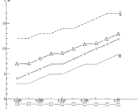
Figure 2 through 7 show the variations of the optimal policy and asso-ciated cost subject to changes in demand rate, production rate, setup cost, backlogging cost, holding cost, and demand size distribution, respectively.

r, Q 15 10 5 " . - - - _ .... ..- ..-5~~~TC---L--,,;&'~--J---~~I~--i---n<~1 ~--i---~L--r~I,---0.045 0.095 0.145 0.195 0.27

0--0--0--0--0--0--0--0--0--0

(14)

r,Q 15 10 5 Production/Invel1tory Problem

6___...

0... f::::.

--Q

...

0~-6

-...:0-0~-6-6.-6.-6.'--....

o - - o - o - o - - o - A

---g

o

_. _. _. I

B

_. I I _lo7I _p.

0 - 0 - 0 - 0 - 0 - 0 - - · - 0 - 0 - 0

Figure 3. The Optimal Policies (r,Q) with Varying ~

r.Q - - - - -Q 15 10 !::;-&.

_--

6.-~0/

h-~·o:"'----___ y-

0:"'----6 . - 0:"'----6 . /

~

0..---

0

_--- ---

Q o~---5 O~~~2~-+4--~3~"'~-L-~4---LI-~~~-~I-~IL--J~.5~~

O-Ci-O-D-O-D-O

Figure 4. The Optimal Policies (r,Q) with Varying K

(15)

146 CS. Sung & G. T. Oh r,Q - -- - - -- - - Q 15 6--6--6--6--6--6--6--6-~--6 0 - 0 0 - 0 - -

o--o~ ~

---o--o~

0 10

---g

5 b

Figure 5. The Optimal Policies (r,Q) with Varying b

r,Q \ 15 10 5-... _ - - - -

----g

~rr_~~I~~I~~~I~~~~~~( - h

D--D--~-0--6-0-6

1.0

-"""""'0-0-0

(16)

r,Q 15 10 5 Production/Inventory Problem ---Q

&"-£1-£1-6

----0~--£1-6--6--6-6

---0--0--0--0

-,-- _. -- --- -- ---9

o

p

Figure 7. The Optimal Policies (r ,Q) with Varying p

147

In these figures, curves connecting symbols lc., 0 and 0 represent Q

O values,

optimal Q values, and optimal r values" respectively, and that both

Q

and

Q

values are described in dotted curves.

From Figures 2 and 3, as the ratio A/)l increases, while r (which reflects the safety stock) does not change. This implies that the expected number of setups remains relatively constant. Figure 4 shows that the setup cost increases, the major policy change is for Q-r to increase, so that a rather long setup interval is required.

Figures 5 and 6 show that as the ratio b/h increases, both rand Q increase. This is interpreted as more inventory holdings are required.

Figure 7 shows that Q decreases as p increases. This is because more frequent setups for production are required to compensate for backloggings.

6. Concl usion

As discussed in Section 4, the major difficulty of the problem is heavily dependent upon the production lot size (or capacity) of Q, since the computa-tional load of determining the associated steady-state probability distribu-tions of 1T and ~ increases enormously Ivith Q.

(17)

(non-instanta-148

c.

neous) setup time can be immediately considered as long as setup times along with production times are defined in convolution.

References

[1] Bailey, N.T.J.: On Queueing Process with Bulk Service. Journal of the Royal Statistical Society Series B, Vol.16 (1954), 80-87.

[2] Bell, C.E.: Characterization and Computation of Optimal Policies for Operating an M/G/l Queueing System with Removable Server. Operations Research, Vol.19 (1971), 208-218.

[3] Cinlar, E.: Introduction to Stochastic Processes. Prentice-Hall, Englewood cliffs, New Jersey, 1975.

[4] Gavish, B. and Graves, S.C.: A One - Product Production / Inventory Problem under Continuous Review Policy. Operations Research, Vol.28

(1980), 1228-1236.

[5] Gavish, B. and Graves, S.C.: Production / Inventory Systems with a Stochastic Production Rate under a Continuous Review Policy. Computers and Operations Research, Vol.8 (1981), 169-183.

[6] Graves, S.C. and Keilson, J.: The Compensation Method Applied to a One -Product -Production / Inventory Problem. Mathematics of Operations Research, Vol.6 (1981), 246-262.

[7] Gross, D. and Harris, C.: Fundamentals of Queueing Theory. John Wiley and Sons, New York, 1974.

[8] Heyman, D.: Optimal Operating Policies for M/G/l Queueing Systems. Operations Research, Vol.16 (1968), 362-382.

[9] Neuts, M.f.: Queues Solvable without Rouche's Theorem. Operations Research, Vol.27 (1979), 767-781.

[10] Orkenyi, P.: Optimal Control of the M/G/l Queueing System with Removable Server Linear and Non-Linear Holding Cost Function. Technical Report No.65, Stanford O.R. Department, August, 1976.

[11] Powell, W.B.: Analysis of Vehicle Holding and Cancellation Strategies in Bulk Arrival, Bulk Service Queues. Report EES-81-12 (Revised), Princeton C.E. Department, February, 1981.

[12] Powell, W.B.: Iterative Algorithms for Bulk Arrival, Bulk Service Queues with Poisson and Non-Poisson Arrivals. Report EES-83-16 (Revised), Princeton C.E. Department, November, 1983.

[13] Powell, W.B., and Humblet, P.: The Bulk Service Queue with a General Control Strategy; Theoretical Analysis and a New Computational Procedure.

(18)

Production/Inventory Problem 149

Report EES-83-5, Princeton C.E. Department, July, 1983.

[14] Schellhaas, H.: Bewertete Regenerative Prozesse mit Anwendung auf Lager-haltungsmodelle mit Zustandsabhangigen Parametern. Preprint Nr.136, Technishe Hochschule Darmstadt, May, 1974.

[15] Sobel, N.J.: Optimal Average Cost Policy for a Queue with Start-up and Shut-down Cost. Operations Research, Vol.17 (1969), 145-162.

Chang Sup SUNG: Dept. of Industrial Engineering, KAIST P.O.Box 150 Cheongryang, Seoul, Korea