Symmetric rank-one method based on some modified secant conditions for unconstrained optimization

(1)

Symmetric rank-one method based on some

modiﬁed secant conditions for unconstrained

optimization

Yasushi Narushima

(Received February 8, 2010; Revised June 18, 2011)

Abstract. The symmetric rank-one (SR1) method is one of the well-known quasi-Newton methods, and many researchers have studied the SR1 method. On the other hand, to accelerate quasi-Newton methods, some researchers have proposed variants of the secant condition. In this paper, we propose SR1 meth-ods based on some modiﬁed secant conditions. We analyze local behaviors of the methods. In order to establish the global convergence of the methods, we apply the trust region method to our methods.

AMS 2010 Mathematics Subject Classiﬁcation. 90C30, 90C53

Key words and phrases. Unconstrained optimization, symmetric rank-one

method, modiﬁed secant conditions, local convergence, trust region method.

§1. Introduction

We consider the following unconstrained minimization problem: (1.1) minimize f (x), f : Rn→ R, x∈ Rn

where f is suﬃciently smooth and its gradient g and Hessian H are available. Quasi-Newton methods for solving (1.1) are iterative methods of the form:

(1.2) xk+1= xk+ sk.

In quasi-Newton methods, the step sk is generated based on an approximation

to the Hessian H(xk), say Bk. Most of quasi-Newton methods generate Bk

which satisﬁes the secant condition:

(1.3) Bk+1sk = yk,

(2)

where yk = g(xk+ sk)−gkand gk= g(xk). There are some updating formulas

for Bk that include the BFGS update, the DFP update and the symmetric

rank-one (SR1) update, for instance.

We do not specify how to compute sk in (1.2). If we use a line search

tech-nique, then sk is deﬁned by sk =−αkB−1k gk, where αk > 0 is an appropriate

stepsize. On the other hand, if we use a trust region technique, then sk is an

approximate solution of the following subproblem:

min s∈Rn g T ks + 1 2s T_B ks subject to ksk ≤ ∆k,

where ∆k > 0 is a trust region radius. In trust region techniques, sk is not

always a “step” but is only an “approximate solution”, and hence we set xk+1 = xk if sk is not appropriate as a step. Thus we should note that (1.2)

is not necessarily satisﬁed in trust region approaches. The SR1 update formula is deﬁned by

Bk+1= Bk+

rkrkT

rT_ksk

,

where rk = yk− Bksk. Many researchers have studied the SR1 method. For

example, Conn et al. [2] showed that the approximate matrix Bk based on the

SR1 update converges to the Hessian at the solution. Khalfan et al. [7] proved the R-superlinear convergence of the SR1 method under mild assumptions. Byrd et al. [1] proposed a quasi-Newton method with the SR1 update based on the trust region technique. There are many other studies on SR1 methods which include [8, 9, 11, 14, 15, 17].

On the other hand, to accelerate quasi-Newton methods, some researchers have proposed variants of the secant condition (1.3) including [5, 10, 16, 18, 19]. In this paper, we treat SR1 update formula based on some modiﬁed secant conditions, and analyze local behaviors of quasi-Newton methods based on those SR1 update formulas.

This paper is organized as follows. In Section 2, we state some modiﬁed secant conditions and give SR1 update formulas based on these modiﬁed secant conditions. In Section 3, we analyze local behaviors of the SR1 methods given in Section 2. In Section 4, in order to establish the global convergence of the methods, we apply the trust region method to the SR1 methods described in Section 2. Finally, in Section 5, preliminary numerical results are given.

In this paper, we use the symbol k · k to denote the usual `2-norm of a

(3)

§2. SR1 update formulas based on modified secant conditions In this section, we consider SR1 update formulas based on some modified secant conditions. To this end, we briefly review those modified secant condi-tions.

Zhang et al. [18, 19] set the equation:

sT_kBk+1sk= sTkyk+ θk,

where

θk= 6(f (xk)− f(xk+ sk)) + 3(gk+ g(xk+ sk))Tsk.

Based on the above equation, Zhang et al. gave a modiﬁed secant condition: (2.1) Bk+1sk = zk, zk= yk+

θk

sT_kuk

uk,

where uk∈ Rn is any vector such that sT_kuk6= 0. If kskk is suﬃciently small,

then we have, for any vector uk satisfying sTkuk6= 0, that

sT_k(H(xk+ sk)sk− yk) = O(kskk3),

sT_k(H(xk+ sk)sk− zk) = O(kskk4).

It follows from these relations that the curvature sT_kBk+1skgiven by any

quasi-Newton update with condition (2.1) approximates the second-order curvature sT_kH(xk+ sk)sk with a higher precision than the curvature sTkBk+1skwith the

condition (1.3) does.

Wei et al. [16] consider another equation: sT_kBk+1sk = sTkyk+ ηk,

where

(2.2) ηk= 2(f (xk)− f(xk+ sk)) + (gk+ g(xk+ sk))Tsk.

Based on the above equation, Wei et al. gave another modiﬁed secant condi-tion:

(2.3) Bk+1sk = zk, zk= yk+

ηk

sT_kuk

uk,

where uk ∈ Rnis any vector such that sTkuk6= 0. Note that the approximation

matrix based on the above secant condition satisﬁes the following relation: f (xk) = f (xk+ sk) + g(xk+ sk)T(−sk) +

1 2(−sk)

T_B

k+1(−sk).

Now we estimate zk in secant conditions (2.1) and (2.3). To this end, we

(4)

Assumption.

A1. The objective function f is twice continuously diﬀerentiable everywhere, and the Hessian H is Lipschitz continuous, that is, there exists a constant L such that

kH(x) − H(y)k ≤ Lkx − yk for all x, y∈ Rn.

Lemma 2.1. Assume that Assumption A1 holds and there exists a positive constant γ such that |sT_kuk| ≥ γkskkkukk > 0 for all k. Then

°° °° ηk sT_kuk uk °° °° ≤ L γkskk 2

holds for any k.

Proof. We ﬁrst note that g(xk+ sk) = gk+

R1

0 H(xk+ tsk)sk dt. Then, from

(2.2) and the mean value theorem, we have, for all k, |ηk| = |2(f(xk)− f(xk+ sk)) + (gk+ g(xk+ sk))Tsk| = ¯¯¯¯2(−gT_ksk− 1 2s T kH(xk+ ξsk)sk) + (2gkTsk+ Z 1 0 sT_kH(xk+ tsk)sk dt) ¯¯ ¯¯ = ¯¯¯¯ Z 1 0 sT_k(H(xk+ tsk)− H(xk+ ξsk))sk dt ¯¯ ¯¯ ≤ kskk2 Z 1 0 kH(xk+ tsk)− H(xk+ ξsk)k dt ≤ Lkskk2 Z 1 0 k(xk+ tsk)− (xk+ ξsk)k dt = Lkskk3 Z 1 0 |t − ξ| dt ≤ Lkskk3,

where ξ ∈ (0, 1), the second inequality follows from the Lipschitz continuity of H, and the last inequality from |t − ξ| ≤ 1. Since we have from |sT_kuk| ≥

γkskkkukk that kukk/|sT_kuk| ≤ 1/(γkskk), the proof is complete.

Let x_∗ be a local solution of (1.1) and, for any i≤ j, deﬁne εi,j = max{kxt− x∗k, kxt+ st− x∗k | i ≤ t ≤ j}.

Then we havekskk ≤ kxk+sk−x∗k+kxk−x∗k ≤ 2εk,k. Hence, by Lemma 2.1,

zk in (2.3) can be estimated by

(2.4) zk= yk+

ηk

sT_kuk

(5)

From the relation θk= 3ηk, zk in (2.1) also can be estimated by

(2.5) zk= yk+

θk

sT_kuk

uk= yk+ O(εk,kkskk).

Li and Fukushima [10] proposed the following Levenberg-Marquardt type secant condition:

(2.6) Bk+1sk= zk, zk= yk+ νksk,

where νk is a positive parameter such that νk= O(kgkk) or O(1). By choosing

νkappropriately, zkTsk> 0 can be ensured. Li and Fukushima show the global

convergence of the BFGS method based on (2.6) for nonconvex unconstrained optimization problems. We assume, in this paper, νk = O(kgkk) to establish

a fast rate of convergence of our modiﬁed SR1 method. Then we can estimate zk in (2.6) by

(2.7) zk= yk+ νksk = yk+ O(kgkkkskk) = yk+ O(εk,kkskk),

where the last equality follows from the relationkgkk = kgk− g(x∗)k and the

Lipschitz continuity of g.

From estimates (2.4), (2.5) and (2.7), we can treat secant conditions (2.1), (2.3) and (2.6) as members of the following uniﬁed secant condition:

Bk+1sk= zk, zk= yk+ qk,

(2.8)

where qk is a vector such that

kqkk ≤ τεk,kkskk,

(2.9)

and τ is a nonnegative constant. Based on the modiﬁed secant condition (2.8), we will construct the modiﬁed SR1 update formula:

Bk+1= Bk+ brkbrkT brT ksk , (2.10)

wherebrk= zk−Bksk. In the paper, we consider the method which uses (2.10)

and zk= yk+ qk with (2.9), and call this method MRS1 (Modiﬁed SR1).

§3. Local behavior of MSR1

In this section, we investigate the local behavior of MSR1. We now make assumptions on the approximate matrices Bk and the sequence of iterates

(6)

Assumption.

A2. There exists a positive constant c1 such that

|brT

ksk| ≥ c1kbrkkkskk > 0

(3.1)

holds for all k.

A3. The sequence {xk} converges to a local solution x∗.

A4. The sequence{sk} is uniformly linearly independent, that is, there exist

a positive constant c2 and positive integers k0 and m such that, for all

k≥ k0, one can choose n distinct indices

k≤ k1 <· · · < kn≤ k + m

with

σmin(Sk)≥ c2,

where σmin(Sk) is the minimum singular value of the matrix

Sk= µ sk1 ksk1k ,· · · , skn ksknk ¶ .

We need the condition (3.1) in the convergence analysis of MSR1. On the other hand, if the condition (3.1) does not hold and if |br_kTsk| is very small,

then we have z_kTsk ≈ sT_kBksk. Hence in actual computations, we can use Bk

instead of Bk+1 if (3.1) does not hold.

We deﬁne here the matrix b H`= Z 1 0 H(x`+ ts`)dt (3.2)

for each `. Recall that the relation y` = bH`s` holds, which will be used in the

sequel. In order to investigate the rate of convergence of the MSR1, we give the following useful lemma (see also [2, Lemma 1] and [7, Lemma 3.1]). Lemma 3.1. Assume that Assumptions A1 and A2 hold. Let {xk} be a

se-quence generated by the MSR1. Then the following statements hold: kzj− Bj+1sjk = 0

(3.3)

for all j and

kzj − Bisjk ≤ 2 c1 (L + τ ) µ 1 + 2 c1 ¶i−j−2 εj,i−1ksjk (3.4)

(7)

where the last inequality used εj,j, εk,k ≤ εj,k. Thus from the induction

Next note from the relation y` = bH`s` that we obtain

|yT

ksj− sTkyj| = |sTk( bHk− bHj)sj| ≤ k bHk− bHjkkskkksjk.

Since it follows from the Lipschitz continuity of H that k bHk− bHjk = °° °°Z₀1(H(xk+ tsk)− H(xj+ tsj))dt °° °° ≤ Z 1 0 kH(xk+ tsk)− H(xj + tsj)kdt ≤ L Z 1 0 kxk+ tsk− xj − tsjkdt ≤ L Z 1 0 (tkxk+ sk− x∗k + (1 − t)kxk− x∗k) dt +L Z 1 0 (tkxj+ sj− x∗k + (1 − t)kxj− x∗k) dt ≤ Lεk,k+ Lεj,j ≤ 2Lεj,k,

(8)

where the third inequality comes from xk+ tsk− x∗ = t(xk+ sk− x∗) + (1−

t)(xk− x∗), we get

|yT

ksj− sTkyj| ≤ 2Lεj,kkskkksjk.

Then, for k≥ j + 2, (3.5) yields |brT ksj| ≤ 2(L + τ)εj,kkskkksjk (3.7) +2 c1 (L + τ ) µ 1 + 2 c1 ¶k−j−2 εj,k−1kskkksjk,

while we have from (3.6) that, for k = j + 1, |brT

j+1sj| ≤ 2(L + τ)εj,j+1ksj+1kksjk.

(3.8)

It follows from (2.10), (3.1) and (3.7) that, for k≥ j + 2, kzj− Bk+1sjk = °° °°zj− Bksj− brkbr T ksj brT ksk °° °° ≤ kzj− Bksjk + |br T ksj| c1kskk ≤ 2 c1 (L + τ ) µ 1 + 2 c1 ¶k−j−2 εj,k−1ksjk + 2 c1 (L + τ )εj,kksjk +2 c1 (L + τ ) µ 1 + 2 c1 ¶k−j−2 εj,k−1ksjk = 4 c1 (L + τ ) µ 1 + 2 c1 ¶k−j−2 εj,k−1ksjk + 2 c1 (L + τ )εj,kksjk.

Since c1 ∈ (0, 1) and k ≥ j + 2 yield 1 ≤ (1 + 2/c1)k−j−2 and 3 < 1 + 2/c1,

and since εj,k−1≤ εj,k, we have, for k≥ j + 2, that

kzj− Bk+1sjk ≤ 4 c1 (L + τ ) µ 1 + 2 c1 ¶k−j−2 εj,kksjk +2 c1 (L + τ ) µ 1 + 2 c1 ¶k−j−2 εj,kksjk = 6 c1 (L + τ ) µ 1 + 2 c1 ¶_k−j−2 εj,kksjk ≤ 2 c1 (L + τ ) µ 1 + 2 c1 ¶k−j−1 εj,kksjk.

(9)

These inequalities give (3.4) for i = k + 1 where k≥ j + 1, and therefore (3.4) follows.

By using Lemma 3.1, we have the next theorem.

Theorem 3.1. Assume that Assumptions A1–A4 hold. Let{xk} be a sequence

generated by the MSR1. Then there exists a positive constant c3 such that, for

all k≥ k0,

kBk+m+1− H(x∗)k ≤ c3εk,k+m,

(3.9)

where k0 and m are positive integers given in Assumption A4. Moreover, we

have

lim

k→∞kBk− H(x∗)k = 0.

(3.10)

Proof. Since we have, from (3.2) and the Lipschitz continuity of H, that k bHj− H(x∗)k ≤ L Z 1 0 kxj+ tsj − x∗k dt ≤ L Z 1 0 (tkxj+ sj− x∗k + (1 − t)kxj− x∗k) dt ≤ Lεj,j

holds for all j ≥ 1, it follows from (2.8) and yj = bHjsj that

kzj− H(x∗)sjk = k( bHj− H(x∗))sj+ qjk

(3.11)

≤ k bHj− H(x∗)kksjk + kqjk

≤ Lεk,k+mksjk + τεk,k+mksjk

(10)

for any j∈ {k, k +1, . . . , k +m}, where M1= L + τ , and the second inequality

used (2.9) and εj,j≤ εk,k+m. Moreover, since (k + m + 1)− j − 2 < m for any

such j, we have from (3.4) that kzj− Bk+m+1sjk ≤ 2 c1 (L + τ ) µ 1 + 2 c1 ¶m εk,k+mksjk (3.12) = M2εk,k+mksjk,

where M2 = _c2₁(L + τ )(1 + 2/c1)m. By (3.11) and (3.12), we obtain, for any

j∈ {k, . . . , k + m}, that k(Bk+m+1− H(x∗))sjk ksjk ≤ kzj− H(x∗)sjk ksjk +kzj− Bk+m+1sjk ksjk (3.13) ≤ (M1+ M2)εk,k+m.

Since (3.13) holds for any j∈ {k1, . . . , kn} (recall Assumption A4), we have

kBk+m+1− H(x∗)k ≤ 1 c2k(Bk+m+1− H(x∗ ))Skk (3.14) ≤ p n c2 max j=k1,...,kn °° °°(Bk+m+1− H(x∗)) sj ksjk °° °° ≤ p n c2 (M1+ M2)εk,k+m,

where the ﬁrst inequality follows from kAk ≤ kASkkkSk−1k and kSk−1k =

1/σmin(Sk)≤ 1/c2 by Assumption A4, the second inequality from

kAk ≤ v u u tXn j=1 kajk2 ≤ √ n max 1≤j≤nkajk,

where aj denotes the jth column of A, and the last inequality from (3.13). The

relation (3.14) implies (3.9) with c3=

p

n(M1+ M2)/c2. Now Assumption A3

implies in turn that εk,k+m tends to zero, and hence (3.10) holds.

We note that Theorem 3.1 implies that Bk is necessarily positive deﬁnite

for all k suﬃciently large if H(x_∗) is positive deﬁnite.

Next we give the Q-superlinear rate of convergence properties of the MSR1. Theorem 3.2. Assume that Assumptions A1–A4 hold. Assume also that H(x_∗) is positive deﬁnite, and that Bk given in (2.10) is nonsingular and

xk+1 = xk + sk with sk = −B_k−1gk for all k suﬃciently large. Then {xk}

(11)

P roof . We have

k(Bk− H(x∗))skk

kskk ≤ kB

k− H(x∗)k.

Therefore, if Assumptions A1–A4 hold, then we obtain from Theorem 3.1 that lim

k→∞

k(Bk− H(x∗))skk

kskk

= 0.

This implies that the Dennis-Mor´e condition (see [4] for example) holds.

There-fore the result holds. 2

§4. MSR1 with trust region method

In the previous section, we considered the local behavior of the MSR1 under the assumption xk → x∗. However this assumption is not necessarily satisﬁed.

In order to establish the global convergence of the method, we need to use globalization techniques like line search methods or trust region methods. The approximation matrix Bkgenerated by (2.10) is not always a positive deﬁnite

matrix, and hence trust region methods are more appropriate to the MSR1 than line search methods.

In this section, we apply the trust region method proposed by Shultz et al. [13] to the MSR1. For this purpose, we give some deﬁnitions. For each iteration, to obtain step sk, we approximately solve the following quadratic subproblem:

min s∈Rnmk(s) = f (xk) + g T ks + 1 2s T_B ks subject to ksk ≤ ∆k,

where ∆k > 0 is the kth trust region radius. The approximate solution sk is

chosen such that

P redk≥ σ1kgkk min{∆k, σ2kgkk/kBkk}

(4.1)

holds for positive constants σ1 and σ2 and such that

whenever kskk < 0.8∆k, then Bksk=−gk,

(4.2)

where P redk is the predicted reduction, which is deﬁned by

P redk= f (xk)− mk(sk).

We also deﬁne the actual reduction by

Aredk= f (xk)− f(xk+ sk).

Now we propose our algorithm, which follows the description of Algorithm 2.1 given by Byrd et al. [1].

(12)

Algorithm TRMSR1.

Step 0. Give x0 ∈ Rn, an initial symmetric matrix B0 ∈ Rn×n, an initial

trust region radius ∆0, ξ ∈ (0, 0.1), τ1 ∈ (0, 1) and τ2 > 1. Set

k = 0.

Step 1. Find a feasible approximate solution sk satisfying (4.1) and (4.2) to

the subproblem: min s∈Rn g T ks + 1 2s T_B ks subject to ksk ≤ ∆k. Step 2. If Aredk P redk

> ξ, then set xk+1 = xk+ sk, else set xk+1 = xk.

Step 3. If Aredk P redk > 0.75, if kskk < 0.8∆k, then set ∆k+1 = ∆k, else set ∆k+1= τ2∆k. Else if 0.1≤ Aredk

P redk ≤ 0.75, then set ∆k+1

= ∆k,

else set ∆k+1= τ1∆k.

Step 4. Update Bk by MSR1 update formula (2.10).

Step 5. Set k = k + 1 and go to Step 1.

Note that Bk is updated in Step 4, even if xk is not updated (i.e. xk+1 =

xk). In [1, p.1028], the following comment is given: “Such updates along failed

directions seem to be necessary to the convergence analysis because if the Hessian approximation is incorrect along such a direction and is not updated along that direction very similar directions could, in principle, be generated repeatedly at later iterations. Such steps would be rejected, resulting in the trust region being reduced at these iterations, potentially keeping it small enough that it would interfere with making a superlinear step even if the Hessian approximation is accurate enough to provide one.”

Now we make the additional assumptions for the global convergence of Algorithm TRMSR1.

Assumption.

A5. The sequence {xk} remains in a closed, bounded, convex set D. The

ob-jective function f has a unique stationary point x_∗, and H(x_∗) is positive deﬁnite.

(13)

A6. The sequence of matrices {Bk} generated by the MSR1 update (2.10) is

bounded, namely there exists a positive constant c4 such that kBkk ≤ c4

holds for all k.

As stated before, note that Algorithm TRMSR1 is a trust region method of the type considered in Byrd et. al. [1], and the diﬀerence between their algorithm and Algorithm TRMSR1 is the update formula of Bkonly. Moreover

the global convergence theorem in Byrd et. al. [1, Theorem 2.1] follows from [13, Theorem 2.2] and its proof does not depend on update formulas of Bk.

Accordingly, we give the following theorem without proof.

Theorem 4.1. Suppose that Assumptions A1, A2, A5 and A6 hold. Let{xk}

be the sequence generated by Algorithm T RM SR1. Then the sequence {xk}

converges to x_∗.

In the rest of this section, we consider the rate of convergence of Algo-rithm TRMSR1. First, we give the following lemma that corresponds to [1, Lemma 2.3].

Lemma 4.1. Let {xk} be a sequence of iterates which converges to the local

solution x_∗, and let skbe a sequence of vectors such that xk+sk→ x∗. Assume

that Assumptions A1, A2, A5 and A6 hold. Then there exists a nonnegative integer K such that for any set of n+1 steps,S = {skj | K ≤ k1 <· · · < kn+1},

there exist an index km with m∈ {2, 3, . . . , n + 1} and M3 such that

k(Bkm− H(x∗))skmk kskmk ≤ M3ε1/n_k₁_,k_n+1, where M3 = 4 " √ n(L + τ ) ( 1 2 + 1 c1 µ 1 + 2 c1 ¶kn+1−k1−2) + c4+kH(x∗)k # . Proof. The proof of this lemma is almost the same as the proof of [7, Lemma 3.2], and we only need to show that, for some positive M4that depends on k1, . . . , kn+1,

k(Bkj− H(x∗))sik

ksik ≤ M4

εk1,kn+1

(4.3)

holds for all j = 2, . . . , n + 1 and i∈ {k1, k2, . . . , kj−1}. Similarly to (3.13), we

have k(Bkj− H(x∗))sik ksik ≤ kzi− H(x∗)sik ksik +kzi− Bkjsik ksik ≤ (L + τ)εk1,kn+1 +2 c1 (L + τ ) µ 1 + 2 c1 ¶kn+1−k1−2 εk1,kn+1,

(14)

which implies (4.3) with M4 = (L + τ )

1 (1 + 2/c1)

kn+1−k1−2ª_.

Next we give a lemma which is obtained by applying Lemma 4.1 in a trust region context, and corresponds to [1, Lemma 2.4]. Its proof is the same as the proof of [1, Lemma 2.4], so we omit the proof.

Lemma 4.2. Suppose that Assumptions A1, A2, A5 and A6 hold. Let{xk} be

the sequence generated by Algorithm TRMSR1. Then there exists a nonneg-ative integer N such that, for any set of p (n < p) steps sk+1, sk+2, . . . , sk+p

with k≥ N, there exists a set Gk of at least p− n indices contained in the set

{i | k + 1 ≤ i ≤ k + p} such that

k(Bj− H(x∗))sjk

ksjk ≤ M5

ε1/n_k+1,k+p,

holds for all j∈ Gk, where

M5 = 4 " √ n(L + τ ) ( 1 2+ 1 c1 µ 1 + 2 c1 ¶p−2) + c4+kH(x∗)k # .

Furthermore, for k suﬃciently large, if j ∈ Gk, then

Aredj

P redj ≥ 0.75.

This lemma implies that, in any set of p steps by Algorithm TRMSR1, there are at least p− n steps accepted by Algorithm TRMSR1, and for which the approximate Hessian is accurate. Now we consider the local behaviors of Algorithm TRMSR1.

Theorem 4.2. Suppose that Assumptions A1, A2, A5 and A6 hold. Let{xk}

be the sequence generated by Algorithm T RM SR1. Then {xk} converges to

x_∗ n + 1 step Q-superlinearly, i.e., lim_k→∞kxk+n+1− x∗k/kxk− x∗k = 0 hold.

Moreover, if Assumption A4 holds and Bk is nonsingular for all k suﬃciently

large, then {xk} converges to x∗ Q-superlinearly.

Proof. The n+1 step Q-superlinear convergence property of Algorithm TRMSR1 can be proven in the same way as Theorem 2.7 in [1]. This theorem is proven by using Lemmas 2.2–2.6 and Theorem 2.1 in [1], and these results do not depend on update formulas of Bk except Lemmas 2.3 and 2.4. We can use our

Lemmas 4.1 and 4.2 instead of Lemmas 2.3 and 2.4 in [1] respectively to prove the n + 1 step Q-superlinear convergence property of our method. Hence we omit the proof and we only prove the second result.

(15)

From Theorems 3.1 and 4.1, limk→∞kBk− H(x∗)k = 0 holds, and hence

limk→∞kBk− bHkk = 0 also holds. Therefore, we have from ξ ∈ (0, 0.1) that

Aredk P redk = g T ksk+1₂sTkHbksk gT ksk+ 1 2sTkBksk > ξ (4.4)

holds for all k suﬃciently large. Thus {xk} is updated by xk+1 = xk+ sk in

Step 2 for all k suﬃciently large. By (4.4) and Lemma 2.2 in [1], there exists a positive constant ∆ such that

∆k= ∆ and kskk < 0.8∆

for all k suﬃciently large, and hence {xk} is updated by xk+1 = xk− B_k−1gk.

Therefore, from Theorem 3.2, the proof of the second result is complete.

§5. Numerical results

In this section, we give some numerical results of Algorithm TRMSR1. We examined the following methods:

BFGS : Algorithm TRMSR1 with BFGS update instead of MSR1, SR1 : Algorithm TRMSR1 with SR1 update (namely zk= yk),

MSR1-1 : Algorithm TRMSR1 with (2.1) and uk = yk−1,

MSR1-2 : Algorithm TRMSR1 with (2.3) and uk = yk−1,

MSR1-3 : Algorithm TRMSR1 with (2.6) and νk= 0.01kgkk.

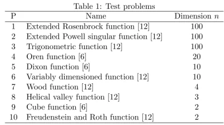
The test problems we used are described in Grippo et al. [6] and Mor´e et al. [12]. In Table 1, the ﬁrst column, the second column and the third column denote the problem number in this paper, the problem name and the dimension of the problem, respectively. For each problem, we used the standard initial point x0 given by [6] and [12].

The program was coded in JAVA 1.6, and computations were carried out on a Dell Precision 490 (Intel Xeon CPU 2.33GHz) with 4.0GB RAM. For these numerical experiments, we set ∆0 = 1, ξ = 0.01, τ1 = 0.5 and τ2 = 2

in Algorithm TRMSR1. We used the identity matrix I as an initial matrix B0, and did an initial sizing. Speciﬁcally, in Step 4 of k = 0, we used ˜B0 =

(sT₀z0/sT0s0)I instead of B0 = I before updating B0. For 1 and

MSR1-2, if |sT_kuk| ≥ 10−15kskkkukk was not satisﬁed, we set zk = yk. Moreover, if

(3.1) with c1 = 10−8 did not hold, then we did not update Bk in Step 4 of

Algorithm TRMSR1.

For solving a subproblem in Step 1, we used Hebden’s method (see Algo-rithm 7.2.1 in [3], for example). In Hebden’s method, if kB−1_k gkk ≥ 0.8∆k,

(16)

Table 1: Test problems

P Name Dimension n

1 Extended Rosenbrock function [12] 100 2 Extended Powell singular function [12] 100 3 Trigonometric function [12] 100

4 Oren function [6] 20

5 Dixon function [6] 10

6 Variably dimensioned function [12] 10

7 Wood function [12] 4

8 Helical valley function [12] 3

9 Cube function [6] 2

10 Freudenstein and Roth function [12] 2

nonlinear equation in µ 1 k(Bk+ µI)−1gkk− 1 ∆k = 0

is solved by the Newton method. We stopped the Newton method if (4.1) with σ1 = 0.1 and σ2= 0.75 was satisﬁed.

The stopping condition was

kgkk ≤ 10−5.

We also stopped the algorithm if the number of iterations exceeds 1000. The numerical results of our experiment are reported in Table 2. The numerical results are given in the form of “the number of iterations / the number of inner iterations”. Note that the number of inner iterations means sum of iterations of the Newton method in Step 1. If the number of iterations exceeds 1000, then we denote “Failed ”.

We see from Table 2 that SR1 and MSR1-3 performed better than the other three methods in these limited numerical experiments: for Problem 1, SR1 outperformed MSR1-3; for Problem 3, MSR1-3 was superior to SR1; and for the other eight problems, MSR1-3 was comparable to SR1.

§6. Concluding remarks

In this paper, we treated SR1 method based on some modiﬁed secant con-ditions (MSR1) and investigated local behaviors of MSR1. In addition, we applied trust region methods to MSR1 to establish its global convergence. Al-though we used trust region methods in this paper, we can also consider MSR1

(17)

Table 2: Numerical results of Algorithm TRMSR1 P n BFGS SR1 MSR1-1 MSR1-2 MSR1-3 1 100 87/54 78/56 42/59 65/23 213/167 2 100 91/5 53/13 73/52 69/29 54/25 3 100 46/0 180/117 85/5 97/32 71/7 4 20 544/2 187/2 183/4 188/2 190/2 5 10 217/116 67/16 Failed Failed 60/14 6 10 23/2 23/2 23/2 24/2 25/2 7 4 89/3 44/43 135/43 35/3 43/44 8 3 12/6 18/24 85/28 95/118 19/27 9 2 73/17 48/33 Failed 68/44 45/30 10 2 42/6 16/4 19/5 17/5 17/4

with line search methods. Since the positive deﬁniteness of the approximation matrix Bk is very important for line search methods, we need to establish

brT

ksk> 0 for all k. By choosing qk appropriately, we may be able to establish

brT

ksk> 0 for all k. It is our further study.

Acknowledgements

The author would like to thank the referee for a careful reading of this paper and valuable comments. The author is supported in part by the Grant-in-Aid for Scientiﬁc Research (C) 21510164 of Japan Society for the Promotion of Science.

References

[1] R.H. Byrd, H.F. Khalfan and R.B. Schnabel, Analysis of a symmetric rank-one trust region method, SIAM Journal on Optimization, 6 (1996), 1025–1039. [2] A.R. Conn, N.I.M. Gould and Ph.L. Toint, Convergence of quasi-Newton matrices

generated by the symmetric rank one update, Mathematical Programming, 50 (1991), 177–195.

[3] A.R. Conn, N.I.M. Gould and Ph.L. Toint, Trust Region Methods, MPS-SIAM

Se-ries on Optimization, Society for Industrial and Applied Mathematics and

Math-ematical Programming Society, 2000.

[4] J. E. Dennis and J.J. Mor´e, A characterization of superlinear convergence and its application to quasi-Newton methods, Mathematics of Computation, 28 (1974), 549–560.

(18)

[5] J.A. Ford and I.A. Moghrabi, Multi-step quasi-Newton methods for optimization,

Journal of Computational and Applied Mathematics, 50 (1994), 305–323.

[6] L. Grippo, F. Lampariello and S. Lucidi, A truncated Newton method with non-monotone line search for unconstrained optimization, Journal of Optimization

Theory and Applications, 60 (1989), 401–419.

[7] H.F. Khalfan, R.H. Byrd and R.B. Schnabel, A theoretical and experimental study of the symmetric rank-one update, SIAM Journal on Optimization, 3 (1993), 1– 24.

[8] C.T. Kelley and E.S. Sachs, Local convergence of the symmetric rank-one itera-tion, Computational Optimization and Applications, 9 (1998), 43–63.

[9] W.J. Leong and M.A. Hassan, A restarting approach for the symmetric rank one update for unconstrained optimization, Computational Optimization and

Appli-cations, 42 (2009), 327–334.

[10] D.H. Li and M. Fukushima, A modiﬁed BFGS method and its global convergence in nonconvex minimization, Journal of Computational and Applied Mathematics, 129 (2001), 15–35.

[11] S. Linping, Updating the self-scaling symmetric rank one algorithm with limited memory for large-scale unconstrained optimization, Computational Optimization

and Applications, 27 (2004), 23–29.

[12] J.J. Mor´e, B.S. Garbow and K.E. Hillstrom, Testing unconstrained optimization software, ACM Transactions on Mathematical Software, 7 (1981), 17–41.

[13] G.A. Shultz, R.B. Schnabel and R.H. Byrd, A family of trust-region-based algo-rithms for unconstrained minimization with strong global convergence properties,

SIAM Journal on Numerical Analysis, 22 (1985), 47–67.

[14] B. Smith and J.L. Nazareth, Metric-based symmetric rank-one updates,

Com-putational Optimization and Applications, 8 (1997), 219–244.

[15] P. Spellucci, A modiﬁed rank one update which converges Q-superlinearly,

Com-putational Optimization and Applications, 19 (2001), 273–296.

[16] Z. Wei, G. Li and L. Qi, New quasi-Newton methods for unconstrained optimiza-tion problems, Applied Mathematics and Computaoptimiza-tion, 175 (2006), 1156–1188. [17] H. Wolkowicz, Measures for symmetric rank-one updates, Mathematics of

Oper-ations Research, 19 (1994), 815–830.

[18] J.Z. Zhang, N.Y. Deng and L.H. Chen, New quasi-Newton equation and related methods for unconstrained optimization, Journal of Optimization Theory and

Applications, 102 (1999), 147–167.

[19] J. Zhang and C. Xu, Properties and numerical performance of quasi-Newton methods with modiﬁed quasi-Newton equations, Journal of Computational and

(19)

Yasushi Narushima

Department of Communication and Information Science Fukushima National College of Technology

30 Nagao, Tairakamiarakawa-aza, Iwaki-shi, Fukushima 907-8034, Japan