Development of microindentation robot for hardness and stiffness measurement with vision based navigation system

全文

(1)Development of microindentation robot for hardness and stiffness measurement with vision based navigation system. Montree PAKKRATOKE Department of Mechanical Engineering and Intelligent systems The University of Electro-Communications. A Thesis submitted for the degree of Doctoral of Engineering 2013 March.

(2) Development of microindentation robot for hardness and stiffness measurement with vision based navigation system. Approved by Supervisory Committee: Chair Person: Prof. Dr. Hisayuki AOYAMA Member: Assoc. Prof. Dr. Chisato KANAMORI Member: Assoc. Prof. Dr. Aiguo MING Member: Assoc. Prof. Dr. Koichi MORISHIGE Member: Assoc. Prof. Dr.Takuji KOIKE.

(3) Copyright2013 Montree PAKKRATOKE All right reserved.

(4) 概要本論文ではマイクロロボットを用いた精密微小硬さ計測システムの開発を目的に、2段平行ばね、VCA、圧子およびLVDTなどから構成される微小力発生検知機構とこれを搭載する超小形精密自走機械および画像計測に基づく経路誘導方法について論じている。本論文では生体材料などの柔らかい材料表面を環境を制御されたチャンバー内で精密に検査することや従来サイズの機構では到達が困難な狭所での検査作業を目標とし、システムの提案、設計試作および基本性能評価を行った。この装置では最大17mNの発生力で50μNの分解能を有すること確認し、さらにシステムに実装し、応用実験を行った。その結果、±3µmの分解能で検査対象に精密誘導し、表面特性を自動連続取得が可能であることを示した。. i.

(5) Abstract A microsurface measurement system that is composed of a microrobot with an indenter, and a vision-based navigation system is proposed for investigating the hardness and stiffness of microparts. The microindentation mechanism is composed of the small force generator mechanism, which is simply combination between a voice coil actuator (VCA) and the tandem leaf spring mechanism. The generated force can be controlled by electrical current, which is supplied to coil and positioned precisely at the balance point with the parallel leaf spring without mechanical friction. And the full bridge strain gauges on both sides of double leaf spring can be detected the small force which is applied to the sample with a microindenter. This handmade small mechanism can produce and verify a small force up to 17 mN with good linearity and 50 µN resolutions. The displacement of the indenter head is measured by a linear variable differential transformer (LVDT) which is included in machine. Thus, this mechanism generates small force and monitors the depth behavior of the indenter during the indentation test. Since the overall mechanism is very small, then it is implemented on the microrobot. The piezo-driven microrobot is capable of moving step by step precisely with 1 µm per step, so the sample surface can be penetrated anywhere by the microindenter. With the benefits of the image processing technique, a vision-based coordination system with a local close-up view and an overall global view has been developed to identify the locations of the robot and the indenter precisely within ±3 µm of accuracy over the working range. The experiment results present the performance of this machine by the surface stiffness investigation of several materials including metal and bio materials. The surface stiffness/hardness was successfully checked, and the indentation load-depth characteristics were precisely acquired. With the surface characteristic results of the certified hardness blocks (30HV and 100HV), the degree of stiffness and hardness can be compared. Finally, the performance of a vision-based navigation system is present on the surface characteristics of the unhealthy human tooth that are precisely acquired at the specified measurement point.. iii.

(6) Contents Page ABSTRACT .......................................................................................................... i. CONTENTS .......................................................................................................... v. LIST OF FIGURES .............................................................................................. ix. LIST OF TABLES ............................................................................................... xix 1 INTRODUCTION .............................................................................................. 1. 1.1 Hardness measurement .............................................................................. 2. 1.1.1 Scratch hardness test ......................................................................... 3. 1.1.2 Rebound hardness test ...................................................................... 5. 1.1.3 Indentation hardness test .................................................................. 8. 1.1.3.1 Macroindentation hardness ..................................................... 8. 1.1.3.1.1 Rockwell Hardness............................................................ 9. 1.1.3.1.2 Vickers Hardness .............................................................. 10. 1.1.3.2 Microindentation hardness ....................................................... 12. 1.1.3.3 Nanoindentation hardness ........................................................ 13. 1.2 Loading method and mechanism of indentation hardness machine ......... 17. 1.2.1 Deadweight type ............................................................................... 17. 1.2.2 Electronic force type ......................................................................... 19. 1.3 Equipment to measure indentation depth ................................................. 22. 1.4 Research motivation ................................................................................. 26. 2 MICROINDENTATION MECHANISM .......................................................... 31. 2.1 System layout and configuration .............................................................. 31. 2.2 Microforce generator mechanism ............................................................. 32. 2.2.1 Design of Voice coil actuator (VCA) ............................................... 32. 2.2.2 Experiment on repulsive force .......................................................... 37. 2.2.3 Experiment on displacement generated ............................................ 39. 2.2.4 Force sensor unit ............................................................................... 41. v.

(7) 2.3 Desplacement sensor for indentation depth of the indenter ..................... 48. 2.4 A combination of microforce generator and depth measuring device ...... 53. 2.5 Heartzian’s contact .................................................................................... 55. 2.6 Gap between the indenter and specimen surface ....................................... 61. 2.6.1 Simulation and boundary conditions ................................................. 61. 2.6.2 Indentation experiments with different indenter gaps ....................... 69. 2.7 Basic performance .................................................................................... 72. 2.8 Discussion .................................................................................................. 75. 3 MICROINDENTATION ROBOT .................................................................... 77. 3.1 Piezo driven inchworm microrobot ........................................................... 77. 3.1.1 Principle and structure design .......................................................... 77. 3.1.2 Robot control algorithm ................................................................... 78. 3.1.3 Robot movement performance test ................................................... 81. 3.2 A combination of microindentation mechanism and microrobot ............. 84. 3.2.1 Assemble of microrobot with small force indenter .......................... 84. 3.2.2 Experiment on mobility of the microrobot ........................................ 88. 3.2.3 Indentation experiment on BIO samples ........................................... 91. 3.2.3.1 Indentation on human nails ...................................................... 91. 3.2.3.2 Indentation on rice grains ......................................................... 96. 3.2.3.3 Indentation on human teeth ..................................................... 102 3.3 Discussion ................................................................................................ 107 4 VISION BASED NAVIGATION SYSTEM FOR ROBOT PATH CONTROL ..................................................................................................... 109. 4.1 Basic Image processing ........................................................................... 110 4.1.1 Image formation .............................................................................. 110 4.1.2 Sampling and quantization .............................................................. 112 4.1.3 Binary image .................................................................................... 114 4.1.4 Image detection ................................................................................ 116 4.2 Robot path control with vision based navigation system ........................ 117 vi.

(8) 4.2.1 Experiment setup for calibration of the camera system .................. 118 4.2.1.1 Calibration in wide-range view ............................................... 120 4.2.1.2 Calibration in microscopic view ............................................. 120 4.2.1.3 The lighting system .................................................................. 123 4.2.2 Robot path control strategies ........................................................... 125 4.2.2.1 Path control for wide working range ....................................... 126 4.2.2.2 Path control for microscopic working range ........................... 129 4.2.3 Basic performance ............................................................................ 131 4.2.3.1 Wide-range path control .......................................................... 131 4.2.3.2 Microscopic range path control ............................................... 132 4.2.3.3 Sample measurement test ........................................................ 135 4.3 Discussion ................................................................................................ 136 5 CONCLUSION AND FUTURE WORK .......................................................... 139 5.1 Conclusion ............................................................................................... 139 5.1.1 Conclusion of chapter 1. ................................................................... 139 5.1.2 Conclusion of chapter 2 .................................................................... 139 5.1.3 Conclusion of chapter 3 .................................................................... 140 5.1.4 Conclusion of chapter 4 .................................................................... 140 5.2 Future work .............................................................................................. 142 REFERENCES..................................................................................................... 145 ACRONYMS ....................................................................................................... 157 PUBLICATIONS ................................................................................................. 159 ACKNOWLEDGEMENTS ................................................................................. 161 BIBLIOGRAPHY ................................................................................................ 163. vii.

(9) List of Figures. 1.1. The relationship between the stress and strain of a material under tension force applied ................................................................................... 1.2. 1. The relationship between hardness and UTS. From the conversion of hardness to hardness or hardness to tensile strength values for unalloyed and low-alloy steels and cast iron [1-1] ...................................................... 1.3. (A) Scratches on the material with different loads. (B) Defining the average of the scratch width [1-4] .............................................................. 1.4. 2. 3. (A) File hardness set 40HRC to 55HRC model TTC HTF-6S [1-5].(B) Pencil hardness set model FMH-5 [1-6]..................................................... 5. 1.5. (A) First two models of EQUOTIP hardness testers. 1975 series. ............. 6. 1.6. (A) Schematic view of the EQUOIP impact device. (B) Typical induction voltage signal generated by the permanent magnet inside the impact body during the main three test phases of an EQUOTIP hardness test [1-7] ...................................................................................................... 7. 1.7. Hardness testing force range....................................................................... 8. 1.8. (A)The Rockwell indenters. (B)The certified hardness blocks .................. 9. 1.9. (A)Rockwell hardness testing cycle. (B) The indentation depth versus a testing force. ............................................................................................... 9. 1.10 (A)Vickers hardness testing cycle. (B)The diagonal of an indentation. .... 11. 1.11 (A) Knoop hardness testing cycle. (B) The Knoop indenter and the indentation. ................................................................................................. 13. 1.12 (A) Berkovich indenter tip. (B) The Berkovich indentation observed by SEM. .......................................................................................................... 1.13 (A) Schematic illustration of indentation load-displacement data showing important measured parameters. (B) Schematic illustration of. ix. 14.

(10) the unloading process showing parameters characterizing the contact geometry [1-18] .......................................................................................... 14. 1.14 Loading mechanism of (A) Rockwell machine and (B) Vickers machine... .................................................................................................... 18. 1.15 (A) Electronic force closed-loop control diagram. (B) Rockwell 2000 series hardness tester from Wilson hardness an Instron company [1-28] .. 19. 1.16 (A) Electronic force loading mechanism for nanoindentation, an electromagnetic actuation.[1-2] (B) The Nano-Indenter G200 from Agilent company[1-31]............................................................................... 20. 1.17 Electronic force loading mechanism for nanoindentation by using (A) electrostatic actuation and (B) the spring-based force actuation[1-33]...... 21. 1.18 (A) Electronic force loading mechanism for nanoindentation by using load trough spring actuation. (B) The spring-based force actuation [1-29] .......................................................................................................... 21. 1.19 The commercial hardness testing machine illustrate the dial gauge, equipment for indentation depth measurement[1-36] ................................ 22. 1.20 (A) Capacitive sensor and (B) the differential capacitor technique for measure the indentation depth [1-31] ......................................................... 23. 1.21 (A) Cutaway view of the LVDT [1-37]. (B) And the differential voltage output varies with core position [1-39] ...................................................... 24. 1.22 The CSM microscratch test, MST employed the LVDT to monitor the penetration depth [1-27] ............................................................................. 24. 1.23 (A)The optical lever method application on cantilever based system [1-29]. (B) Laser interferometer setup to measure the indentation depth.. 25. 1.24 The hardness calibration machine employed laser interferometer to measure the indentation depth [1-40] ......................................................... 25. 1.25 Approximately size comparison between the commercial type hardness machine and the original microsurface investigation robot. The robot aim to operate inside small chamber. ........................................................ x. 27.

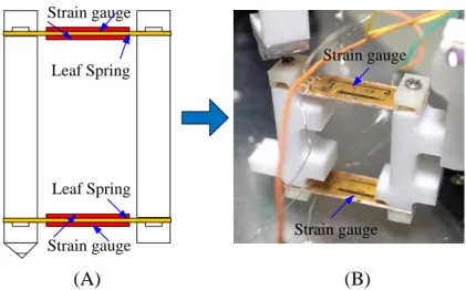
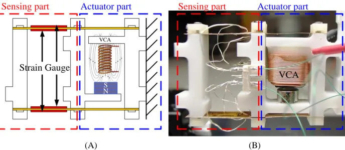
(11) 1.26 Microdiagnostics robot with hardness and stiffness testing navigation based on multiple vision images................................................................. 28. 1.27 On-site service for underground pipeline inspections. .............................. 28. 2.1. Layout of the microindentation mechanism, (A) Actuator part, (B) Sensor part and (C) the combination layout between (A) and (B). ........... 2.2. 31. Cutaway picture of a sound speaker, demonstrates the voice coil (solenoid coil) and a permanent magnet layout [2-1]................................. 32. 2.3. Layout of the actuator part.......................................................................... 33. 2.4. Parallel leaf spring parameters. .................................................................. 35. 2.5. (A) Solenoid coil in actions when supplied the current. (B) The fabricated solenoid coil. .............................................................................. 2.6. Experiment setup for determining the repulsive force between solenoid and permanent magnet, (A) Setup diagram and (B) Equipment setup....... 2.7. 36. 37. Repulsive force between solenoid and permanent magnet (dash line from calculation, and solid line from primary experiment) of each current supply, compare with the design value of main structure spring constant and the force generated experiment results of the fabricated VCA. ........................................................................................................... 2.8. 2.9. 38. The fabricated voice coil actuator (VCA) associated with tandem parallel leaf spring. ..................................................................................... 39. Control diagram of the solenoid coil. ......................................................... 40. 2.10 Experiment results with the displacement of the paralleled spring driven by VCA. ...................................................................................................... 40. 2.11 Experiment results with the step response to the input current. ................. 41. 2.12 The force sensor unit associated with tandem parallel leaf spring, (A) diagram layout and (B) the fabricated unit. ................................................ 42. 2.13 The schematic diagram of force sensor unit, composed of bridge amplifier (DA-710A), the multimeter (Agilent 34411A) and PC. ............ xi. 42.

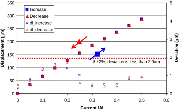
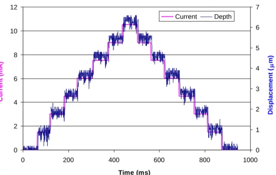
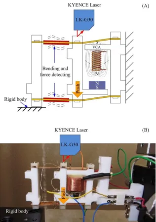
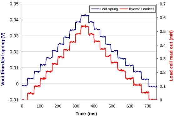
(12) 2.14 The force sensor unit associated with tandem parallel leaf spring, (A) diagram layout and (B) the fabricated unit. ................................................ 43. 2.15 Feedback control diagram of a microforce generator mechanism. ............ 43. 2.16 (A) Schematic diagram and (B) Experiment setup for determined the basic performance of a sensor part after attached to the actuator part. ...... 44. 2.17 Experiment result of small step movement. ............................................... 45. 2.18 Experiment result of large step movement. ................................................ 45. 2.19 (A) Schematic diagram and (B) Experiment setup for generated force verification. ................................................................................................. 46. 2.20 Experiment results with the relation between the generated force and the displacement. The force comparison between standard load cell and output from leaf spring with 20 measurements in uncontrolled room temperature. ................................................................................................ 46. 2.21 Experiment results with the resolution of the generated force. .................. 47. 2.22 Overall system control block diagram. ....................................................... 48. 2.23 (A) The LVDT coil is removed from the micrometer head. (B) Wire holder to prevent the fragile LVDT wires. (C) The LVDT inside an enclosure package. ...................................................................................... 49. 2.24 Experiment setup for LVDT performance test. .......................................... 49. 2.25 (A) Comparison result between LVDT and Laser displacement. (B) Close up data shows the same behavior of both devices. ........................... 51. 2.26 Calibration results of LVDT by using Laser displacement sensor. Red squares are the results of each calibration point. Blue circles are the deviation at each calibration point. ............................................................. 52. 2.27 (A) Diagram layout and (B) fabricated of the prototype of microhardness machine. ............................................................................. 53. 2.28 The testing cycle behavior of indentation depth from LVDT readout and the application force from strain gauge. It is separated by region A to F for each status. .................................................................................... xii. 54.

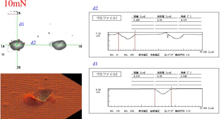
(13) 2.29 Contact between a rigid sphere and the flat surface.[2-11]. ....................... 55. 2.30 Comparison between the calculation results and measurement results of the indenter circle contact with various testing force on 30HV gold block............................................................................................................ 57. 2.31 Comparison between (A) the theoretical heartzian’s contact and (B) the practical measurement. ............................................................................... 58. 2.32 Indentation profile on gold block surface with 5mN testing force. ........... 59. 2.33 Indentation profile on gold block surface with 10mN testing force. ......... 59. 2.34 Indentation profile on gold block surface with 15mN testing force. ......... 60. 2.35 Indentation profile on gold block surface with 20mN testing force. ......... 60. 2.36 Boundary conditions of the simulation....................................................... 62. 2.37 FEA mesh for the indenter gap simulation. The number of nodes and elements are 87,550 and 52,945 respectively. ............................................ 62. 2.38 FEA simulation result at 0µm indenter gap (A) without deform and (B) with deformed result. .................................................................................. 63. 2.39 Close up view at the indentation contact point with 0µm indenter gap FEA simulation result, (A) without deform and (B) with deformed result............................................................................................................ 64. 2.40 FEA simulation result at 100µm indenter gap (A) without deform and (B) with deformed result............................................................................. 65. 2.41 Close up view at the indentation contact point with 100µm indenter gap FEA simulation result, (A) without deform and (B) with deformed result............................................................................................................ 66. 2.42 FEA simulation result at 40µm indenter gap (A) without deform and (B) with deformed result............................................................................. 67. 2.43 Close up view at the indentation contact point with 40µm indenter gap FEA simulation result, (A) without deform and (B) with deformed result............................................................................................................ xiii. 68.

(14) 2.44 Indentations 3D Profile on 30HV block with different test force and different indenter gaps. ............................................................................... 70. 2.45 30HV and 100HV certified hardness blocks. ............................................. 72. 2.46 Indentation 3D profile of 30HV compare with 100HV. ............................ 73. 2.47 Indentation load-depth curve of 30HV certified block at 5mN, 10mN and 15mN testing force............................................................................... 74. 2.48 Indentation load-depth curve of 100HV certified block at 5mN, 10mN and 15mN testing force............................................................................... 74. 3.1. Diagram picture and photo of the original inchworm microrobot. ............ 77. 3.2. Control diagram for inchworm robot. ........................................................ 77. 3.3. PZT and electromagnetic legs control timing diagram for forward direction. ..................................................................................................... 3.4. PZT and electromagnetic legs control timing diagram for backward direction. ..................................................................................................... 3.5. 79. PZT and electromagnetic legs control timing diagram for turn right direction. ..................................................................................................... 3.6. 78. 80. PZT and electromagnetic legs control timing diagram for turn left direction. ..................................................................................................... 80. 3.7. Experiment setup for robot movement performance test. .......................... 81. 3.8. Resolution experiment result on step movement of the microrobot. 3.9. (measured in four times forward and backward directions). ...................... 81. Experiment setup for repeatability test. ...................................................... 82. 3.10 Repeatability experiment on step movement of microrobot. Measured in four directions, Forward (FW), Backward (BW), Turn right (TR) and Turn left (TL). ............................................................................................. 83. 3.11 Solidwork design of a microindentation robot. .......................................... 84. xiv.

(15) 3.12 Design of the adjustable cantilever mechanism (hanger) which is unable to adjust the angle of a measurement part. (A) normal state and (B) liftup position. ................................................................................................. 85. 3.13 The prototype of the microindentation robot.............................................. 86. 3.14 Control diagram of the microindentation robot. ......................................... 87. 3.15 (A) Artificial sample with small defect. (B) The schematic diagram presents the robot path walks through the pipe. ......................................... 88. 3.16 The robot walk through the pipe, start from the bottom right to the bottom left. .................................................................................................. 89. 3.17 Indentation load-depth curves present the problem area on a glue hole with very deep indentation depth compare with normal sample surface. .. 90. 3.18 Cross section of the nail structure [3-6]. .................................................... 92. 3.19 Finger nail sample were clipped in 22 mm and placed on plastic plate by epoxy glue. ............................................................................................. 92. 3.20 Indentation load-depth curves of each sample group. ................................ 93. 3.21 Mean of group the indentation load-depth curves from each group. ......... 94. 3.22 3D profile of the indentation on human finger nail. ................................... 95. 3.23 Outer layers and internal structures of rice grain[3-14]. ............................ 96. 3.24 Rice grains are placed on the substrate with epoxy dry fast glue. ............. 97. 3.25 3D profile of the indentation on rice grains................................................ 97. 3.26 Indentation load-depth curves of Japanese rice uncooked and cooked. ..... 98. 3.27 Indentation load-depth curves of sticky rice uncooked and cooked. ......... 99. 3.28 Indentation load-depth curves of Thai rice uncooked and cooked............ 100 3.29 Mean of group of the indentation load-depth curves of rice grain, here the letter R is the representative of “raw or uncooked”, the letter C means “cooked”. ........................................................................................ 101 3.30. Diagram of human tooth [3-15]. ............................................................... 102. 3.31 Anatomy of a tooth [3-17]. ........................................................................ 103. xv.

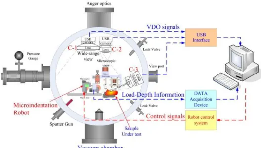
(16) 3.32 Two incisors teeth samples (milk teeth and permanent teeth) before cut (Left). The teeth were placed on substrate by epoxy glue (Right) with polished surface. ........................................................................................ 104 3.33 (A) The milk tooth and (B) the permanent tooth with vertical cut and indentation in transverse.3D image from laser scanning microscope of the indentations on (C) milk tooth and (D) permanent tooth. ................... 104 3.34 Indentation load-depth curves of milk tooth. ............................................ 105 3.35 Indentation load-depth curves of permanent tooth. ................................... 106 3.36 Mean of group of indentation load-depth curves of permanent tooth and milk tooth compare with load-depth curves of certified hardness block. . 106 3.37 The series of indentions under manual position control............................ 107 4.1. Microdiagnostics robot with hardness and stiffness testing, navigation based on multiple vision images................................................................ 109. 4.2. Diagram of an electronic camera [4-2] ...................................................... 111. 4.3. Diagram of the human eye [4-2]................................................................ 111. 4.4. Representation of digital images by arrays of discrete points on a rectangular grid: (A) 2-D image (B) 3-D image [4-3]............................... 112. 4.5. Effect of different sampling rates [4-4] ..................................................... 113. 4.6. Effect of different quantization levels [4-4] .............................................. 113. 4.7. The example of a Binary image converts from color image [4-6] ............ 115. 4.8. Thresholding of grayscale image [4-8]...................................................... 115. 4.9. Template matching example, (A) Array of objects and (B) Triangle template...................................................................................................... 116. 4.10 The prototype of the microindentation robot............................................. 117 4.11 Multi-cameras based coordinate system for robot navigation................... 118 4.12 Experiment setup for calibration of cameras pixel change compare with the actual movement of X-Y controlled stage (A) wide-range view and (B) microscopic view. ................................................................................ 119. xvi.

(17) 4.13 Comparison results between actual movement of a marker and a pixel change of C2 camera (wide-range view). .................................................. 120 4.14 Comparison results between actual movement of a marker and a pixel change of C1 camera (microscopic view). ................................................ 121 4.15 The vision based navigation system of the microindentation robot with three CCD cameras in the chamber. .......................................................... 122 4.16 Camera views and the actual scale from C1, C2 and C3 in the chamber.. 122 4.17 The lighting system. (A) External light for wide-range camera. (B) The internal ring light for microscopic view camera. (C) Overall lighting system. ....................................................................................................... 123 4.18 The marker ant its score at several positions around the working area..... 124 4.19 Measurement process algorithms .............................................................. 125 4.20 Robot path design algorithm for wide working range (C2 camera). ......... 127 4.21 Turning angle and Y-displacement ability of the robot which is monitored by C2 camera............................................................................ 128 4.22 Robot path design algorithm for microscopic working range (C1 camera)....................................................................................................... 129 4.23 Experiment setup for wide-range path control. ......................................... 131 4.24 Repeatability experiment results of wide-range path control.................... 132 4.25 Experiment setup for microscopic range path control. (In this picture is shown the marker that placed on the top of LVDT case. .......................... 133 4.26 Repeatability experiment results of microscopic range path control. ....... 133 4.27 The robot during automatically reaches the target with different starting position i.e., (A) below the center line and (B) above the center line. ...... 134 4.28 (A) Artificial defects on a human tooth. (B) The designed paths on a glue hole of a human tooth. (C) The series of indentations scan pass through the glue hole on dentin surface of a human tooth. ....................... 135. xvii.

(18) 4.29 3D indentation load-depth curves present the problem area on a human tooth with very deep indentation depth compare with normal tooth surface. ....................................................................................................... 136 4.30 The improvement of the indentation pattern before (up) and after (down) implemented the vision-based navigation system. ....................... 137. 5.1. (A) The previous model with non-symmetric structure and (B) the new design with symmetric structure ................................................................ 143. xviii.

(19) List of Tables 2.1. Calculation results and measurement results on the indenter circle contact ......................................................................................................... 57. 2.2. Effect of the indenter gap on each test force .............................................. 71. 2.3. Diameter of indentation compare with maximum depth from load-depth curve............................................................................................................ xix. 74.

(20) CHAPTER 1. INTRODUCTION Material selection in engineering applications is crucial. Engineers have to confirm that material properties are appropriate for the operational condition. There are many kinds of material properties, and ultimate tensile strength is one of the most useful for predicting the strength of a material. The tensile test is a fundamental materials science test in which a sample is subjected to uniaxial tension until failure. It can be predicted the strength of materials, which the maximum stress on the stress-strain curve (UTS) is the point that the material under test can be withstood before damage.. Figure 1.1 The relationship between the stress and strain of a material under tension force applied. The relationship between the stress and strain of a material under tension force applied is shown in Fig. 1.1 most of the material display linear elastic behavior from the pulling point A up to a proportional limit point B. At this region the deformations are completely recoverable upon removal of the load. That is a specimen loaded elastically in tension will elongate, but after unloaded it will return to the original shape and size. Pass this linear region, the deformation of metal materials still elastic but no longer linear. The deformed specimen will not return to its original size and shape when unloaded. For many applications, when a material passed a proportional limit deformation, it is unacceptable and cannot be used. At this point is used as the safety design 1.

(21) limitation. After the yield point C, the deformation of ductile materials is plastic. It is gone over a period of strain hardening. That is a stress increases again with increasing strain, and they begin to a neck shape. When necking becomes substantial, it causes a reversal of the stress-strain curve, i.e., it is calculated assuming the original cross-sectional area before necking. The reversal point is the maximum stress on the stress-strain curve, and the stress coordinate of this point is the ultimate tensile strength (UTS), given by point D. The UTS is used for quality control, because of the ease of testing. It is also used to roughly determine material types for unknown samples. However, in tensile testing method, the test material is destroyed, which means that such testing is not appropriate in some situations. In addition, there is another way to predict the strength of a material without greatly damaging a test sample that is the hardness test. In Fig. 1.2 has shown the relationship between hardness and ultimate tensile strength, it is nearly proportional each other.. Figure 1.2 The relationship between hardness and UTS. From the conversion of hardness to hardness or hardness to tensile strength values for unalloyed and low-alloy steels and cast iron [1-1]. 1.1 Hardness measurement The hardness test has been widely used for nearly 100years because indentations are very small and the surface quality of the material is not destroyed. This technique is therefore considered as nondestructive test method. 2.

(22) Hardness is not the physical parameter like length, time, mass, electric current; it is the industrial parameter or the comparative value same as other mechanical characteristics. The Metals Handbook defines hardness as "Resistance of metal to local plastic deformation”, usually by indentation. However, the term may also refer to stiffness or temper or to resistance, to scratching, abrasion, or cutting. It is the property of a metal, which gives it the ability to resist being permanently, deformed (bent, broken, or have its shape changed), when a load is applied [1-2]. This is the usual type of hardness test, in which rounded indenter is pressed into a surface under a substantially static load. There are three general types of hardness measurements as follows. 1.1.1 Scratch hardness Scratch hardness test (Fig. 1.3) is the resistance of solid surfaces to permanent deformation under the action of a single point (diamond stylus tip) [1-3]. It is a companion method to quasi-static hardness tests in which a stylus is pressed into a surface under a certain normal load and the resultant depth or impression size is used to compute a hardness number. Scratch hardness numbers involve a different combination of properties of the surface because the indenter (diamond stylus) moves tangentially along the surface. Therefore, the stress state under the scratching stylus differs from that produced under a quasistatic indenter. Scratch hardness numbers are in principle a more appropriate measure of the damage resistance of a material to surface damage processes like two-body abrasion than are quasi-static hardness numbers.. (A). (B). Figure 1.3 (A) Scratches on the material with different loads. (B) Defining the average of the scratch width [1-4]. 3.

(23) Before the measurements, the indenter shape is calibrated on a reference sample using the series of scratches at several defined loads. The material hardness value is calculated in comparison to the reference hardness as a proportion between the loads and widths of scratches on both the tested and reference materials. The scratch hardness value is expressed as the load in kilograms divided by the square of the width of the scratch in millimeters as follows Eq. (1.2) [1-4]. ….……………………………..(1.1) ………………………………(1.2) Where; H is hardness. b is scratch width (mm). P is normal load (kgf). k(b) is the calibration function. This test method is applicable to a wide range of materials. These include metals, alloys, and some polymers. The main criteria are that the scratching process produces a measurable scratch in the surface being tested without causing catastrophic fracture, spallation, or extensive delamination of surface material. Severe damage to the test surface, such that the scratch width is not clearly identifiable or that the edges of the scratch are chipped or distorted, invalidates the use of this test method to determine a scratch hardness number. Since the degree and type of surface damage in a material may vary with applied load, the applicability of this test to certain classes of materials may be limited by the maximum load at which valid scratch width measurements can be made.. 4.

(24) (A). (B). Figure 1.4 (A) File hardness set 40HRC to 55HRC model TTC HTF-6S. [1-5] (B) Pencil hardness set model FMH-5 [1-6]. Other methods for scratch hardness determination include the use of hardness standards for scratching plastics such as hardness-graded pencils (kohinoor value), minerals of known hardness (mohs value) falling carborundum particles (Fig. 1.4). 1.1.2 Rebound hardness test Rebound hardness test [1-7] or Leeb rebound hardness test is a dynamic hardness testing. It is determined by the action when making an object collides with the test surface and the rebound height is measured. This type of hardness is related to elasticity. The device used to take this measurement is known as scleroscope and Shore hardness. The rebound hardness test method was developed in 1975 by Leeb and Brandestini at Proceq SA (the Switzerland company who is a developer, manufacturer and distributor of portable instruments for nondestructive testing of material properties) to provide a portable hardness test for metals. It was developed as an alternative to the unwieldy and sometimes intricate traditional hardness measuring equipment. The first rebound product on the market was named “Equotip” as shown in Fig. 1.5 a dynamic hardness test method and instrument. The traditional hardness measurements likes Rockwell or Vickers are set up in segregated testing areas or laboratories of plants. Samples are cut off from selected parts and measured in the laboratory. It was required to test a very large piece or pieces that are unwieldy to be tested in the usual types of testing machines no alternative was 5.

(25) (A). (B). Figure 1.5 (A) First two models of EQUOTIP hardness testers. 1975 series, and (B) series of red hexagonal EQUOTIP, produced between 1978 and 1990 [1-7]. available. Testing parts of fixed structures, or testing under any conditions which require that the indentation force be applied in a direction other than vertical, made the search for portable solutions indispensable. Such hardness testers were initially limited to field tests where the test piece could not be brought to the testing instrument. Meanwhile the portable Leeb rebound hardness mainly used as a portable hardness tester. An impact device shown in Fig. 1.6(A) containing a permanent magnet and the very hard sphere shape indenter facing towards the surface of the test material. The velocity of the impact body is recorded in three main test phases; First, the pre-impact phase, where the impact body is accelerated by spring force towards the surface of the test piece. Second, the impact phase, where the impact body and the test piece are in contact. The hard indenter tip deforms the test material elastically and plastically and is deformed itself elastically. After the impact body is fully stopped, elastic recovery of the test material and the impact body takes place and causes the rebound of the impact body. Finally, the rebound phase, where the impact body leaves the test piece with residual energy, not consumed during the impact phase. The Leeb method idea was to measure the velocity of the impact body contact-free via the induction voltage generated by the moving magnet trough a defined induction coil mounted on the guide tube of the device.. 6.

(26) (A). (B). Figure 1.6 (A) Schematic view of the EQUOIP impact device. (B) Typical induction voltage signal generated by the permanent magnet inside the impact body during the main three test phases of an EQUOTIP hardness test [1-7]. The induced voltage is directly proportional to the velocity of the magnet, thus, the impact body containing the magnet. The induced induction signal shown in Fig. 1.6(B) is recorded in an electronic indicator device and the peak induction voltages are further processed to give Leeb.s hardness number, the Lvalue. The shape of the induction signal is unique for each device type. The Lvalue, also known as Leeb-number or Leeb hardness(HL), is simply described as equal to the ratio of the rebound velocity vr to the impact velocity vi of the impact body, multiplied by 1000 as shown in Eq.1.3. ……………………………….(1.3) The specified impact body represents by impact velocity, impact body mass and overall elasticity the penetration stressing and in form of the rebound velocity vr the materials response to this penetration. Thus, all information on hardness is available and the L-value is a suitable and direct measure for materials hardness. However, the Leeb hardness test is a superficial determination only measuring the condition of the surface contacted. The results generated at that location do not represent the part at any other surface location and yield no information about the material at subsurface locations [1-8]. 7.

(27) 1.1.3 Indentation hardness test The Indentation hardness test is determined from the dimension of permanent deformation on the test surface and testing force that makes the deformation. By one of the most common methods of hardness testing (Rockwell), hardness is determined by the depth of the indentation in the test material resulting from application of a given force on a specific indenter. In the Brinell and Vickers hardness test, hardness is determined by the impression created by forcing a specific indenter into the test material under a specific force for a given length of time. It depends on the time of loading, the temperature and other operating conditions. The indentation hardness tests can be divided from testing force into three classes as shown in Fig. 1.7 the macroindentation, microindentation and the nanoindentation test. Permissible error (N) 30. Macro Force. 10 Brinell Hardness. 5. 1.9kN – 30kN. Rockwell Hardness 600N – 1.5kN. 1 0.1. Vickers Hardness. 0.01 0.001. 100N – 1kN. Micro Force Micro Vickers 0.1N – 2N. Our machine 50µN – 20mN. Nano Force. 0.0001. Lower than 2N. 30. 10. 5. 1. 0.01. 0.001. 0.0001. 0.1. 0. Test Force (kN). Figure 1.7 Hardness testing force range. 1.1.3.1 Macroindentation hardness. The macroindentation is applied to tests with a larger test load, such as 1 kgf or more. There are various macroindentation tests such as Vickers hardness test (HV), Brinell hardness test (HB), Knoop hardness test (HK), Meyer hardness test, Rockwell hardness test (HR) and Shore hardness test.. 8.

(28) 1.1.3.1.1 Rockwell hardness The Rockwell hardness testing method is forcing an indenter (diamond cone steel or hard metal ball) into the surface of test piece in two steps under specified conditions. The Rockwell indenter and the Rockwell hardness block are shown in Fig. 1.8. The Rockwell hardness can be determined by measured the permanent depth h of indentation under preliminary test force after removal of additional test force [1-9].. (A). (B). Figure 1.8 (A) The Rockwell indenters. (B) The certified hardness block. The general Rockwell test procedure is shown in Fig.1.9 at first, the indenter is approached the material surface with a preliminary force (F0) applied. Then hold the constant force for a period of time (dwell time). After that, the indentation depth is mark as a reference first position. Then an additional force is applied to increase the applied force to the total force level (F). The total Force (N). F. Depth (µm) Additional force application time. Total force dwell time. h. Preliminary force dwell time. Recovery dwell time. F0 Increasing Time(s). (A). F0. F. Force (N). (B). Figure 1.9 (A) Rockwell hardness testing cycle. (B) The indentation depth versus a testing force. 9.

(29) force is held constant for a set of time period, after that the additional force is removed. The test force returned to the preliminary force level. After holding the preliminary force constant a set time period, the indentation depth is measured for a second position. Finally, removed the indenter from the test material. The deviation between the first and second indentation depth position, h is then used to calculate the Rockwell hardness number. The Rockwell hardness number is calculated from the difference in the indentation depths before and after application of the total force, while maintaining the preliminary test force. The difference in indentation depths is measured as h(in mm). The calculation of the Rockwell hardness number is dependent on the specific combination of indenter type and the forces that are used. For Rockwell scales that use a sphere conical diamond indenter; the regular Rockwell hardness, i.e., HRA, HRC, HRD and the Rockwell Superficial Hardness, i.e., HR15N, HR30N, HR45N is calculated from Eq. 1.4 and 1.5, respectively. ……..…………(1.4) ……..……….…(1.5) For scales that use a ball indenter; the regular Rockwell hardness, i.e., HRB, HRE, HRF, HRG, HRH, HRK and the Rockwell Superficial Hardness, i.e., HR15T, HR30T, HR45T is calculated from Eq. 1.6 and 1.7, respectively. ……..…………(1.6) ……..………....(1.7) 1.1.3.1.2 Vickers hardness The Vickers hardness test was developed in 1921 by Robert L. Smith and George E. Sandland at Vickers Ltd. It can be used for all metals and has one of the widest scales among hardness tests. It is mostly used for small parts and thin sections. The Vickers hardness is based on as optical measurement. The basic principle is forced a diamond indenter in the form of a right pyramid with the square base and with a specified angle between opposite faces at the vertex into the surface of a test piece. Then measured the diagonal length of the indentation on the test piece surface after removed the indenter. Finally, the average of 10.

(30) Force (N) Additional Force Application Time. Applied test force F(N). 136O. Test force dwell time. F d1. d. d2. (A). Increasing time (s). (B). Figure 1.10 (A) Vickers hardness testing cycle. (B) The diagonal of an indentation. diagonal lengths is used to calculate the Vickers hardness number [1-10]. The HV number is then determined by the ratio F/A where F is the force applied to the diamond in kilograms-force and A is the surface area of the resulting indentation in square millimeters. A can be determined by the equation as follows: (. ⁄ ). ………………………..…(1.8) …………………………….……..(1.9). Where; F is the testing force (N). d is an arithmetic mean of the two diagonals length d1 and d 2 (mm) When the mean diagonal of the indentation has been determined the Vickers hardness may be calculated from the formula, but is more convenient to use conversion tables. The Vickers hardness should be reported like 800HV/10, which means a Vickers hardness of 800, was obtained using a 10kgf force. Several different loading settings give practically identical hardness numbers on uniform material, which is much better than the arbitrary changing of scale with the other hardness testing methods. The advantages of the Vickers hardness test are that extremely accurate readings can be taken, and just one type of indenter is used for all types of metals and surface treatments. Although thoroughly adaptable and very precise for testing the softest and hardest of materials, under 11.

(31) varying loads, the Vickers machine is a floor standing unit that is more expensive than the Brinell or Rockwell machines. The Vickers hardness can be converted in SI units (MPa or GPa) by multiply 9.807 for HV to MPa, and multiply 0.009807 for HV to GPa. 1.1.3.2 Microindentation hardness The microindentation tests [1-11, 1-12] typically have forces up to 2N and produce the indentations about 50μm. It has been widely employed in the literature to describe the hardness testing of materials with low applied loads. It can be used to observe changes in hardness on the microscopic scale. Unfortunately, it is difficult to standardize microhardness measurements, i.e., it has been found that the microhardness of almost any material is higher than its macrohardness. Additionally, microhardness values vary with load and workhardening effects of materials [1-13]. A basic principle of a microhardness is impressed a diamond indenter of specific geometry into the surface of the test specimen using a known applied force from 1 to 1000 grams force (gf). The hardness number is based on the surface area of the indentation divided by the applied force, a hardness units in kgf/mm² can be given. The two most commonly used as a microhardness tests are the Vickers hardness test (HV) and the Knoop hardness test (HK). The Knoop hardness test was developed by at the National Bureau of Standards (NIST) in 1939[1-14]. The indenter used is a pyramidal diamond that produces an elongated diamond shaped indentation. It is particularly used for very stiff materials or thin sheets, because the elongated pyramid only creates a shallow impression. The basic principle is pressed the pyramidal diamond indenter into the polished surface of the test material with a known force, for a specified dwell time, normally 10 - 15 seconds. The tests are mainly done at test forces from 10gf to 1000gf, so a high powered microscope is necessary to measure the resulting indentation size. After the dwell time is complete, the indenter is removed leaving an elongated diamond shaped indent in the sample. The size of the indent is determined optically by measuring the longest diagonal of the diamond shaped indentation. The Knoop hardness number is a function of the test force divided by the projected area of the indent. The diagonal is used in the following formula to calculate the Knoop hardness. The geometry of this indenter is an extended pyramid with the length to width ratio being 7:1 and 12.

(32) respective face angles are 172 degrees for the long edge and 130 degrees for the short edge as shown in Fig. 1.11(B). The depth of the indentation can be approximated as 1/30 of the long dimension [1-15]. The Knoop hardness HK or KHN is then given by the equation as follows: ………………..…….(1.10) Where; L is the length of indentation along its long axis(mm). Cp is the correction factor related to the indenter geometry and the units of force and diagonal, ideally 0.070279. P is the testing force (kgf)[1-16]. The Knoop number normally ranges from HK60 to HK1000 for metals, will increase as the sample gets harder. A typical Knoop hardness is specified as 650HK0.5, where; 650 is the calculated hardness. 0.5 is the test force in kg. Force (N) Additional Force Application Time. Test force dwell time. F. (A). Increasing time (s). (B). Figure 1.11 (A) Knoop hardness testing cycle. (B) The Knoop indenter and the indentation. 1.1.3.3 Nanoindentation hardness The nanoindentation [1-17, 1-18] techniques used to obtain mechanical properties from very small volumes of material. This method was developed to measure the hardness and elastic modulus of a material from indentation load– displacement data obtained during one cycle of loading and unloading. Nanoindentation test typically have forces lower than 2N. It is originally applied with the Berkovich triangular pyramid indenter as shown in Fig. 1.12. However, Oliver and Pharr [1-18] have realized that it can be applied to a variety of axisymmetric indenter geometries including the sphere. A schematic depiction 13.

(33) (A). (B). Figure 1.12 (A) Berkovich indenter tip. (B) The Berkovich indentation observed by SEM. of a typical data set obtained with a Berkovich indenter is shown in Fig. 1.13(A) where the parameter P defines the testing load and the displacement h qualified to the initial un-deformed surface. During loading, the deformation is supposed to be both elastic and plastic as the permanent hardness impression forms. It is assumed to be only the elastic displacements are recovered during unloading. The deformation of the material under test is the elastic natures of the unloading curve. There are three important quantities that must be measured from the P-h curves, i.e., the maximum load Pmax, the maximum displacement hmax, and the. (A). (B). Figure 1.13 (A) Schematic illustration of indentation load–displacement data showing important measured parameters. (B) Schematic illustration of the unloading process showing parameters characterizing the contact geometry [1-18]. 14.

(34) elastic unloading stiffness S = dP/dh. There are defined as the slope of the unloading curve during the first stages of unloading (also called the contact stiffness). The accuracy of hardness and modulus measurement depends on how well these parameters can be measured. Another important quantity is the final depth hf, the permanent depth of penetration after the indenter is fully unloaded. The analysis used to determine the hardness H, and elastic modulus E, is principally the method proposed by Doerner and Nix [1-19]. Their method is less complicated because it is a linear curve fit of the selected minimum to maximum data. However, it is limited because the calculated elastic modulus will decrease as more data points are used along the unloading curve. The Oliver-Pharr [1-18] nonlinear curve fit method to the unloading curve data is usually well approximated as the power law relation given by:. (. ) …………………………..(1.11). Where; h is the variable depth. hf is the final depth.  and m are power law fitting constants. The exact procedure used to measure H and E is based on the unloading processes shown in Fig. 1.13(B). It is assumed that the behavior of the Berkovich indenter can be modeled by a conical indenter with a half-included angle , that gives the same depth to area relationship  =70.3°. The basic assumption is that the contact edge sinks-in manner can be described by models for indentation of a flat elastic half space by rigid indentions on a simple geometry [1-20 to 1–28]. However, this assumption is only described the sinksin behavior at the contact edge. It does not define the pile-up of material at the contact edge, which is occurred in some elastic–plastic materials. Assuming that pile-up is negligible, the elastic models that show the amount of sink-in hs, is given by:. ………………..………………(1.12) Where;.  is a constant, which depends on the geometry of the indenter. 15.

(35) Using Eq. (1.12) to approximate the vertical displacement of the contact edge, it follows from the geometry shown in Fig. 1.12(B). That the depth along the contact area is made between the indenter and the specimen hc = hmax − hs, is: ………………………(1.13) Assuming that F(d) is an area function (the indenter shape function) describes the cross sectional area of the indenter at a distance d back from its tip, the contact area A is: ……………………………….(1.14) This function must carefully be calibrated because the deviations from non-ideal indenter geometry are caused the accuracy of the contact area. These deviations can be quite severe near the Berkovich indenter tip, where some rounding predictably occurs during the grinding process. Although a basic procedure for determining the area function was presented as part of the Oliver-Pharr’s original method [1-25], new improved [1-18] have made significant changes to it in recent years. The hardness can be given by the equation below, relating the maximum load to the indentation area. ……………..………………….(1.15) This definition of hardness may deviate from the traditional hardness measured, if there is significant elastic recovery during unloading. Because the relation is based on the contact area under load applied not the residual hardness impression. However, this is dominate only in extremely small values of E/H materials [1-26]. The slope of the curve, dP/dh, upon unloading is indicative of the stiffness S of the contact can be given by: √. √ …………………………(1.16). Where; β is a geometrical constant. In the original method for measuring hardness and modulus, the dimensionless parameter β was taken as unity. A is the projected area of the indentation. Eeff is the effective elastic modulus defined by …………………………..(1.17). 16.

(36) Where; Ei and i is the elastic modulus and the poisson’s ratio of the indenter, for diamond indenter tip Ei is 1140 GPa and i is 0.07. The Poisson’s ratio of the specimen s, generally varies between 0 and 0.5 for most materials and is typically around 0.3. The nanoindentation technique has been widely used to evaluate mechanical properties of materials at the micro and nano-scale, especially hardness and elastic modulus. It can be used to characterize organic, inorganic, soft or hard materials and coatings. Examples are thin and multilayer PVD, CVD, PECVD, photoresists, paints, lacquers, and many other types of films and coatings. Bulk material surface mechanical characterization can also be performed on hard or soft materials, including metals, semiconductors, glasses, ceramics, composites, biomimetic and in vitro biomaterials. The accuracy and precision of the data are assured by having the lowest thermal drift currently available of any nanoindentation [1-27].. 1.2 Loading methods and mechanism of indentation hardness machine One of the most important parameters in any hardness machines is the loading method and the mechanism of the machine. The loading mechanism and force sensor have been improved significantly over the last 20 years. There are two typically type of the loading method used in recent day, the deadweight type and the electronic force type. The deadweight type is the most accurate and high long term stability of the generated force. However, for a very low force scale (lower than 2N) is very difficult to control, because the friction is dominate. Each loading method might suitable for another hardness testing method described as follows. 1.2.1 Deadweight type The traditional hardness testers employ the deadweight systems. It is very simple and reliable method to apply and hold the testing force. With respect to operating convenience, deadweight type does not require a power source and can generate a stable and precise output pressure to be applied. Especially, if high testing force range is required. The deadweight system utilizes a series of 17.

(37) incremental, stacked weights in conjunction with a lever and pivot point to apply a magnified test force at the indenter. Minor loads are applied by spring or small weight. The loading methods of hardness machines are different as forces necessary for various hardness testing methods are different. In general, the hardness machines are built for the different testing methods, such as; Rockwell, Vickers or Brinell. As shown in Fig. 1.14 is the principle of a deadweight Rockwell and Vickers machine. The Rockwell testing method (60, 100 and 150kgf) differ from the Vickers (187.5kgf) and Brinell (3000kgf) by employing a preliminary test force. The Vickers and brinell machines are required only a single force step. Deadweight type have been performing hardness indentations since the Rockwell hardness test was developed in and are still a popular and efficient way to perform a hardness test. In general, deadweight type is more precise devices providing very low uncertainties based on percent of reading rather than full scale. However, for a very large force hardness test methods are not a problem to of the deadweight application, but for very low force hardness test methods likes Microvickers, Knoop or nanoindentation (lower than 2N), the spring or counter weight have are required. This counter weight might cause a mechanical friction and may the source of pour generated force long term stability. It also very difficult to control applying the weights in a deadweight system. To apply the test force, the weight has to be moved, and stopping it quickly without overload and oscillation creates a problem. Recently, the Loading Lever Pushing rod. Loading Metal Microscope. Weight support Weights. Turret turning knob. Load changing rod. Indenter. Weight Disk. Table Load changing dial Elevating Shaft Loading speed adjusting. Hand Wheel. Load Handle. (A). (B). Figure 1.14 Loading mechanism of (A) Rockwell machine and (B) Vickers machine 18.

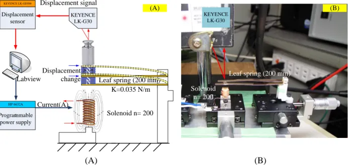
(38) electronic force generator techniques have been developed as an alternative method of load application. Moreover, it is very difficult to make such nanoindentation test force with the deadweight type. 1.2.2 Electronic force type The electronic force is an innovator technology that utilizes motor/encoder control and a load cell or force transducer to apply and regulate the load. It can constantly monitor and adjust the applied force. Moreover, eliminating force errors and increasing tester accuracy and repeatability. The closed-loop control schematic diagram shown in Fig. 1.15(A) is a very simple generated and controlled force system. It is composed of the microcontroller that controls an actuator drives the indenter which is attached at the end of loadcell down to the specimen. It means that during applying force, the indentation force can be monitored and controlled in the same time. As shown in Fig. 1.15(B) the electronic force hardness tester from Wilson hardness an Instron company. This Rockwell machine can generate force from 3kgf up to 150kgf with very small overall structure.. (A). (B). Figure 1.15 (A) Electronic force closed-loop control diagram. (B) Rockwell 2000 series hardness tester from Wilson hardness an Instron company [1-28]. Regarding to the nanoindentation hardness [1-29] there are various mechanisms and methods that have been designed to complete nanoindentation hardness tests. One method of force application was introduced by Pethica [130] in 1983. The basic principle is using a coil and a permanent magnet assembly on a loading column to drive the indenter downward as shown in Fig. 19.

(39) (A). (B). Figure 1.16 (A) Electronic force loading mechanism for nanoindentation, an electromagnetic actuation.[1-2] (B)The Nano-Indenter G200 from Agilent company[1-31]. 1.16(A). This configuration looks familiar the driver from an audio speaker, voice coil actuator (VCA). By varying the current (I), through the coil, a magnetic field is generated that interacts with the magnetic field of the permanent magnet. The loading column is suspended by springs, which damps external motion and allows the load to be released slightly to recover the elastic portion of deformation before measuring the indentation depth. In Fig. 1.16(B) is shown the commercial nanoindentation machine from Agilent Company, the Nano-Indenter G200. This machine using the electromagnetic actuation that can produce the testing force up to 10N (required high load option) with 50nN generated force resolution. Another force actuation method using the electrostatic force was proposed by Lilleodden et al [1-32] in 1995. The basic principle mechanism structure is shown in Fig. 1.17(A). In this method the test force is produced by an electrostatic force generated between the center plate and the upper or lower plate of a three-plate transducer system, i.e., by applied AC signals 180° out of phase with each other to the top and bottom plate. The applied load is proportional to the square of the voltage, the AC signals are picked up by the center (floating) plate and the sum of the signals corresponds to a displacement of the plate. To apply a load, a DC voltage offset is applied to the lower plate of the transducer that electrostatically attracts the center (floating) plate downward [1-33]. In Fig. 1.17(B) is shown the commercial nanoindentation machine from Hysitron Company, the TI 950 TriboIndenter. This machine using an electrostatic actuation that can produce the testing force from 30nN up to 10N (with dual head option) with 1nN resolution. 20.

(40) (A). (B). Figure 1.17 Electronic force loading mechanism for nanoindentation by using (A) electrostatic actuation and (B) the spring-based force actuation [1-33]. (A). (B). (C). Figure 1.18 (A) Electronic force loading mechanism for nanoindentation by using load trough spring actuation. (B) The spring-based force actuation. (C) The long range piezo driver and elastic element [1-29]. Another method for produces force is the application of load through spring technique. The indenter shaft and the indenter tip are attached and support by spring while the displacement actuator generates pushing force as shown in Fig. 1.18(A). In 1989, Burnham and Colton [1-34] were propose another actuation by using a piezo actuator incorporates with a set of crossed wires as shown in Fig. 1.18(B). The indenter is supported by double crossed cantilever beam (tungsten wire) and push down by the piezo actuator pass through the scanning tunneling microscopy (STM). In 1992, Bell et.al [1-35] was proposed another approach technique by using the load trough spring method. As shown in Fig. 1.18(C) the indenter shaft and the indenter tip is attached with long range piezo driver and an elastic element. When the indenter is moved downward by the piezo driver, the elastic element resists the movement and creates a force. 21.

(41) Not only an electronic force type able to constantly measure the test force being applied, but the components used in this type inherently advance themselves to a much simpler design than those in a dead-weight type. As mentioned, dead-weight systems require levers, pivots and other frictioninducing components to function efficiently (see Fig. 1.14). On the other hand, an electronic force system’s main component is a load cell or stain gauge. This compact, low-weight device provides an electronic output proportionate to the force applied to it. With this design, sources of error between the indenter and the test force are eliminated. For example, friction in the actuator is so excessive that the desired force is not applied to the indenter, i.e., the load cell constantly checks itself to make certain that only the correct test forces are applied to the indenter. Even though, the electronic force type is very easy to control the generated force. It may be used in place of deadweight type because they may be cheaper and offer more portability. However, deadweight type still provides advantages that must be considered. Moreover, deadweight testers are generally less susceptible to environmental temperature effects on performance accuracy.. 1.3 Equipment to measure indentation depth Another influence factor for hardness measurement is the depth measuring device [1-29], because high accuracy of the depth measurement provides high position of hardness value. The lever actuated dial gauge employed for indentation depth measurement on commercial Rockwell hardness testers (Fig. 1.19). Meanwhile, most Rockwell standardizing machines were employed the. Figure 1.19 The commercial hardness testing machine illustrate the dial gauge, equipment for indentation depth measurement[1-36]. 22.

(42) measuring microscopes for measuring indentation depth. For Vickers and Brinell machines, the indentation depth during an indenting process is not necessary, because the hardness value from these methods are the dimensions size of the indentation. The nanoindeatation described a hardness value by the relation between indentation depth and impressed force during an indentation process. The high accuracy and resolution depth measuring device required to be used. The capacitive sensor technique shown in Fig. 1.19(A) is one of the high resolution displacement measurements. The basic structures composed of two capacitors with three metal plates are placed with a small gap between them and a voltage is applied to the plates, an electric field will exist between the plates. This electric field is the result of the difference between electric charges that are stored on the surfaces of the plates. The amount of existing charge determines how much current must be used to change the voltage on the plate. The capacitance between two plates is determined by the plates size, a gap size and the material between plates (dielectric). In practically capacitive sensor, the plates size and the dielectric material (air) remain constant. The only variable is the gap size. Based on this assumption, the different between C1 and C2 are results of the gap size. The capacitive sensor technique can provides high precision of displacement with very small foot print. As shown in Fig. 1.20(B) is the layout of nanoindentation machine employed with capacitive gauge for measure the indentation depth. [1-37] Another displacement sensor commonly used is the linear variable differential transformer (LVDT) [1-38]. The principle layout is shown in Fig. 1.21(A). It composed of three coils, a primary coil (A) placed at centered. C1. d.  C2. d. (A). (B). Figure 1.20 (A) Capacitive sensor and (B) the differential capacitor technique for measure the indentation depth [1-31]. 23.

(43) A. B1. B1. VOUT = V1 - V2 = 0. VOUT = V1 - V2. B2. A. B1. B2. A. B2. VOUT = V2 - V1. B1. A. CORE. CORE. CORE. Max. LEFT. NULL. Max. RIGHT. (A). B2. (B). Figure 1.21 (A) Cutaway view of the LVDT [1-38]. (B) And the differential voltage output varies with core position [1-39]. between a pair of secondary coils (B1 and B2), symmetrically spaced about the primary. The cylindrical ferromagnetic core moving inside those coils, attached to the object whose position is to be measured. In Fig. 1.21(B) [1-39] when the LVDT's core is in different axial positions, current is driven through the primary coil with a constant amplitude AC source causing an induction current to be generated through the secondary coils, B1 and B2. The magnetic flux thus developed is coupled by the core to the nearby secondary coils, B1 and B2. If the core is located midway between B1 and B2, equal flux is coupled to each secondary so the voltages, V1 and V2, induced in coils B1 and B2 respectively, are equal. At this reference midway core position, known as the null point, the differential voltage output, (V1 - V2), is essentially zero. Besides, if the core is moved closer to B1 than to B2, more flux is coupled to B1 and less to B2, so the induced voltage V1 is increased while V2 is decreased, voltage output is resulting in the differential voltage (V1 - V2). On the other hand, if the core is moved closer to B2, more flux is coupled to B2 and less to B1, so V2 is increased as V1 is decreased, voltage output is equal to (V2 - V1). When compare between LVDT and Capacitance gauge, the measurement range of the LVDT is larger. However, the capacitance gauge has better measurement resolution. In Fig. 1.22 LVDT Displacement sensor. Reference Fork Sample. Figure 1.22 The CSM microscratch test, MST employed the LVDT to monitor the penetration depth [1-27] 24.