Research Center for Price Dynamics
Research Center for Price Dynamics
A Research Project Concerning Prices and Household Behaviors
Based on Micro Transaction Data
Working Paper Series No.12
The Impact of the Great East Japan Earthquake on Commodity Prices:
New Evidence from High-Frequency Scanner Data
Naohito Abe, Chiaki Moriguchi,
and
Noriko Inakura
March 31, 2014
Research Center for Price Dynamics
Institute of Economic Research, Hitotsubashi University
Naka 2-1, Kunitachi-city, Tokyo 186-8603, JAPAN
Tel/Fax: +81-42-580-9138
E-mail:
rcpd-sec@ier.hit-u.ac.jp
http://www ier hit-u ac jp/~ifd/
http://www.ier.hit-u.ac.jp/~ifd/
The Impact of the Great East Japan Earthquake on Commodity Prices:
New Evidence from High-Frequency Scanner Data
*Naohito Abe, Hitotsubashi University Chiaki Moriguchi, Hitotsubashi University
Noriko Inakura, Osaka Sangyo University (from April 1, 2014)
March 31, 2014
Using high-frequency point-of-sales data, we investigate the impact of the Great East Japan Earthquake on prices. In contrast to the official Consumer Price Index that shows little impact, our price index based on scanner data reveals a modest yet notable increase in within-store commodity prices following the disaster in eastern Japan. We find that the disaster had a large and lasting effect in reducing the frequency and magnitude of bargain sales at retail stores especially in Tokyo.
However, under severe commodity shortages, the standard index based on within-store same-commodity price changes may not capture the actual changes in the cost of living. To overcome this problem, we propose two alternative price indices based on (1) commodity price without distinguishing stores and (2) unit price without distinguishing commodities (i.e., brands) within the same category. Focusing on the food categories for which the disaster induced large excess demand, we find that rise in the alternative price indices was considerably greater than that in the standard price index. We further show that observed price elasticity between stores (as well as between brands) declined significantly after the disaster, indicating that, in the face of commodity shortages, the same commodity sold at different stores (or even different brands within the same category) became closer substitutes for consumers.
Keywords: natural disaster, commodity shortages, consumer price index, scanner data JEL classification codes: D22, D40, E31, Q54
* We would like to thank INTAGE Inc. and Nikkei Media Marketing for making their data available for this research. Financial support from the JSPS Grant for the Social Scientific Survey of the Great East Japan Earthquake and the JSPS Grants-in Aid for Young Scientists (S) 21673001 is gratefully acknowledged.
1. Introduction
The Great East Japan Earthquake of March 2011 not only devastated towns and villages in the northeastern region of Japan, but also affected economic activities of millions of firms and consumers far beyond the disaster-stricken area. Most notably, the disaster induced large excess demand for a number of goods, resulting in widespread commodity shortages — symbolized by empty shelves and long queues in supermarkets — in eastern Japan. The excess demand was caused by both demand-side and supply-side shocks. On the demand-side, household expenditure rose sharply after the disaster as consumers tried to stockpile essential goods (e.g., batteries, water, and rice) to cope with the greater future uncertainty (Abe, Moriguchi and Inakura 2013). On the supply-side, due to electric power shortages and the damage to production facilities, the supply of certain goods (e.g., milk and yogurt) declined sharply after the disaster for weeks. Under such circumstances, we may expect the disaster to have had major impacts on commodity prices.
Due to methodological difficulty and data limitations, however, we have remarkably little knowledge about the effect of natural disasters on prices in general. It is often argued that major disasters such as hurricanes, floods, and earthquakes cause a sharp increase in the prices of essential goods and services, much to the detriment of consumers (Sandel 2009; Rotemberg 2011). In the U.S., as many as 31 states have passed anti-price gouging laws that prohibit sellers from raising prices during states of emergency (Davis 2008). These arguments, however, are based largely on anecdotal evidence, as there has been little empirical research on the effects of natural disasters on prices. An important exception is Cavallo et al. (2013) who analyze changes in prices and product availability following the 2010 earthquake in Chile and the 2011 earthquake in Japan. Using daily data collected from online supermarkets, they find that, in both Chile and Japan, product availability declined sharply after the earthquake while prices remained stable. Although innovative and insightful, their data come from a few major online supermarkets whose representativeness can be seriously questioned. Therefore, the first objective of this paper is to investigate the impact of a natural disaster on commodity prices using large-scale and comprehensive scanner data.
The second objective is to propose a new price index that can better capture the cost of living when consumers face severe commodity shortages. We claim that a standard price index (such as the official Consumer Price Index) based on within-store same-commodity prices is an inadequate measure under such circumstances, because a set of available commodities varies greatly both across stores and over time. In fact, as we show below, the number of
commodities sold at retail stores declined dramatically in the week following the disaster in eastern Japan and recovered gradually with an inflow of new commodities. To measure the actual cost of living, it is therefore important to incorporate the effects of high commodity turnover. We propose two alternative price indices in this paper. The first index is based on the average commodity price without distinguishing stores, which can capture changes in commodity prices arising from a shift of demand across stores as consumers search multiple stores to find the commodity under severe shortages. The second index is based on “unit price” defined by the average price per weight, aggregating all commodities (i.e., brands) in the same category.1 This index can capture price increase arising from “higher substitution” where consumers purchase a similar but more expensive commodity when the desired commodity is not available.
Here are the main findings of our paper:
1) In contrast to the official Consumer Price Index (CPI), which shows little change, a price index based on daily scanner data reveals that food prices in eastern Japan increased by 3% in the weeks following the disaster.
2) This rise in within-store commodity prices was driven mainly by changes in bargain sale patterns. The disaster had especially a large and lasting effect in reducing the frequency and magnitude of bargain sales in the Tokyo metropolitan area.
3) When we focus on the four food categories for which there was large excess demand after the disaster, within-store commodity prices increased by 10–20% in the disaster-stricken area, 5–10% in eastern Japan, and 0–5% in western Japan.
4) The price rise in eastern Japan was 5–17% when measured by the index based on across-store commodity prices and10–30% when measured by the index based on unit prices. 5) Our empirical analysis shows that price elasticity between stores as well as between commodities declined significantly after the disaster. This is consistent with our hypothesis that the same commodity sold at different stores — or even different commodities within the same category — became closer substitutes for consumers in the face of commodity shortages. The rest of the paper is structured as follows. In Section 2, we briefly describe scanner data and define geographic areas that we use in a subsequent analysis. In Section 3, we study the impact of the disaster on prices using daily scanner data and examine the role of bargain sales. In Section 4, we propose alternative price indices. In Section 5, we empirically estimate price elasticity of demand between stores and between commodities. Section 6 presents the conclusion of this study.
2. Scanner Data and Geographic Areas of Comparison
In this study, we use two sets of point-of-sales (POS) scanner data: Nikkei-POS and INTAGE-POS2. In Table 1, we summarize the characteristics of our datasets. As a reference, we also summarize Retail Price Survey data (from which the official CPI is computed).
Our first dataset comes from Nikkei Digital Media and contains daily transaction data of more than 160,000 commodities in 156 categories of processed foods from a national sample of approximately 200 retail stores in Japan.3 For each transaction, we observe a date, a unique commodity identifier (i.e., Japanese Article Number code), sales and quantity sold (from which we compute commodity price), and a store code and location. While the commodity coverage of Nikkei-POS is extensive (for example, there are 995 commodities in the category of “cup noodle”), retail stores in the sample are restricted to supermarkets (including general merchandize stores, GMS). We take advantage of the daily frequency of Nikkei-POS data to analyze patterns of bargain sales at retail stores.
Our second dataset is provided by INTAGE, which contains weekly transaction data from a nationally representative sample of nearly 1,900 retail stores in Japan. Although INTAGE-POS covers only four categories of food, namely, cup noodle, bottled water, yogurt, and natto (fermented soybeans, a Japanese traditional staple and an acquired taste), it has the following merits. First, because the number of stores in the sample is large, we can analyze commodity prices in the disaster-stricken area. Second, it covers a wide variety of retail stores including convenient stores that substantially increased their market share after the disaster. Third, its commodity coverage is even more extensive than that of Nikkei-POS (e.g., 1,304 commodities in the category of “cup noodle”). Last but not least, it contains detailed commodity information including physical volume, which enables us to compute a unit price (i.e., price per gram).
In the following analysis, in an effort to isolate the effects of the disaster, we compare three geographical areas of Japan that were differentially affected by the Great East Japan Earthquake (see Figure 1). 1) “Directly Damaged Area (DAA)” consists of 4 prefectures that received major damages from the earthquake, tsunami, and nuclear power plant failures (Iwate,
2 The official name of INTAGE-POS is INTAGE SRI (Retail Panel Survey).
3 Nikkei-POS data do not include fresh foods with no barcodes (e.g., meet, fish, and vegetables). For more details about Nikkei-POS data, see Abe and Tonogi (2010), Handbury et al. (2013), and Sudo et al. (2014).
Miyagi, Fukushima, and Ibaraki). 2) “East” consists of 5 prefectures in greater Tokyo area. The area escaped a direct blow but experienced major tremors of seismic intensity greater than three during March 11-24 (Tokyo, Kanagawa, Yamanashi, Gunma, and Saitama)4. 3) “West” consists of prefectures to the west of Mie except Okinawa. This area experienced no major tremors during the same period. We use “West” as our control, although some commodity shortages were of nationwide phenomena.
3. The Impact of the Great East Japan Earthquake on Consumer Price Index 3.1 Comparing the Official CPI and the CPI based on POS Data
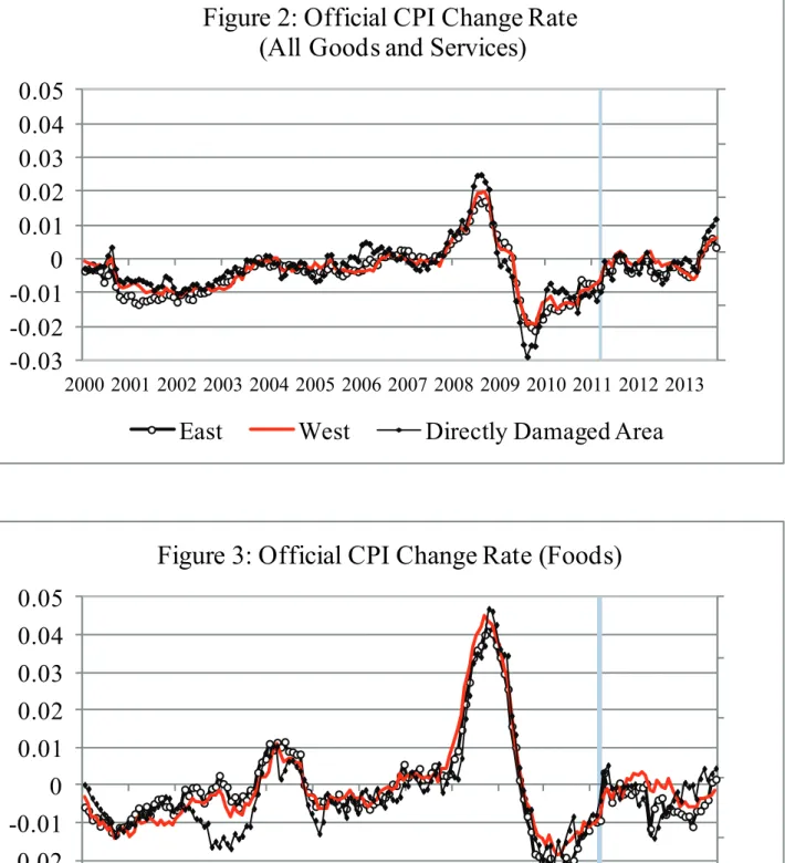
Before turning to our scanner data, we first examine the effects of the disaster on prices as captured by the official Consumer Price Index (CPI) compiled by the Statistics Bureau of Japan based on the monthly Retail Price Survey. In Figure 2, we show the rate of change (from the same month in previous year) in the official CPI for all goods (excluding fresh foods) in DAA, East, and West, from 2000 to 2013. The large increase in 2008 is due to a rise in oil and material prices. From this figure, the impact of the March 2011 disaster (marked as a gray vertical line) is hardly discernable.
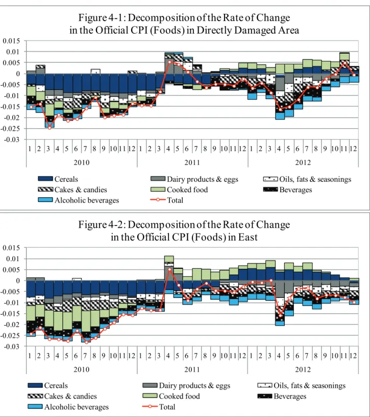
In the following analyses, we restrict the sample categories to foods (excluding fresh foods) to make it comparable to Nikkei-POS data. Figure 3 depicts the rate of change in the official CPI for foods in the three areas. There are visible spikes in April 2011 in East and DAA, but not in West.5 In Figures 4.1-4.3, for each geographical area, we show the decomposition of the rate of change in the official CPI for foods into seven major categories. In both DAA and East, a rise in the prices of dairy products and eggs was a leading factor in increasing the index. In DAA and East, the official food price index increased from March 2011 to April 2011 by 1.3 and 1.7 percentage points, respectively, while in West it rose by 0.6 percentage points.
To summarize, according to the official CPI, the Great East Japan Earthquake had a very limited impact on commodity prices even in the disaster-stricken area. However, as the Boskin Report has pointed out, the official CPI suffers from potentially serious biases in measuring the cost of living (Jorgenson et al. 1996; Jorgenson 2006; Shiratsuka 1999). Compared to the
4 We exclude Chiba from our “East” because about ten thousands of buildings were
severely damaged by the disaster, while in Tokyo, only 11 buildings were damaged. See the damage report by the Ministry of Health, Labour and Welfare,
(http://www.mhlw.go.jp/topics/bukyoku/kenkou/suido/houkoku/suidou/dl/111101_2syou _Part4.pdf).
5 Because the Retail Price Survey in March 2011 was conducted during March 9-11, the official CPI on March 2011 likely represents the pre-disaster price level.
official CPI, a CPI based on Nikkei-POS data has several major advantages (Abe and Tonogi 2010). First, because our data contain information on quantity, we can compute the Fisher index that is free from the upward bias found in the Laspeyres index used in the official CPI. Second, while our CPI based on the daily scanner data incorporates bargain sale prices, the official CPI disregards bargain sales information.6 Third, compared to the official CPI, which is based on a small number of representative commodities, our CPI is less likely to exhibit the “lower substitution” bias because of its extensive commodity coverage (see Table 1).7
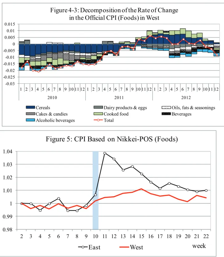
In Figure 5, we present a weekly CPI for foods (excluding fresh foods) based on Nikkei-POS data using the Fisher index.8 The label of the horizontal axis is the week number in 2011 where we take Week 2 as the base week and drop Week 1 (January 3-9) from our sample period as it includes new-year holidays in Japan. Because the day of the earthquake, March 11 (Friday), corresponds to the fifth day of Week 10, the early effects of the disaster are captured in Week 10. In East, food prices increased by 3 percentage points in Week 11 alone, compared to a mere 0.2 percentage point increase in West.9
3.2 Role of Bargain Sales in Price Increase
Compared to the official CPI, our POS-based CPI shows a greater impact of the disaster on within-store commodity prices in eastern Japan. What are the sources of this discrepancy? Even though the official CPI by construction does not reflect changes in bargain sales, changing the frequency or magnitude of bargain sales can be an important means of price adjustments for retail stores.10 We thus investigate the role of bargain sales in the observed price increase after the disaster.
Because Nikkei-POS data do not have an explicit identifier of bargain sales, it is necessary to use a filter to identify such sales. Following Abe and Tonogi (2010), for a given commodity at
6 According to the CPI manual (ILO 2004), the official CPI is based on the prices that do not change for at least seven days. If a sizable number of consumers purchase commodities when they are on sale, then the official CPI overestimates the actual cost of living.
7 According to the CPI manual (ILO 2004), to construct the official CPI, the official survey collects prices of representative commodities sold at representative stores in each survey district. The lower substitution bias occurs when consumers shift their demand from the representative commodities or stores to other commodities or stores with lower prices.
8 The results are essentially the same if we use the GEKS index proposed by Ivanovic et al. (2011) instead of the Fisher index.
9 We cannot compute a CPI for the Directly Affected Area due to a small sample size.
10 Using Nikkei-POS data, Abe and Tonogi (2010) find that the official CPI in Japan in the 2000s exhibits a serious upward bias due to its exclusion of bargain sale prices. An increasing number of papers also emphasize the importance of bargain sales in explaining price stickiness and business cycles (e.g., Midrigan 2011). For an opposing view, see Nakamura and Steinsson (2008).
a given store on a given date, we define “regular price” as the mode price in the past seven days (an alternative definition of the past six weeks is also used below). If a price is lower than the regular price, it is identified as “bargain price.” Using this definition, as a measure of the frequency of bargain sales, we compute the share of commodities sold at a bargain price at each store weighted by sales. Figure 6 shows the average ratio of bargain sales in East and West from February 2010 to October 2012. In East, the ratio of bargain sales declined from 19% in early March 2011 to 13% in early April 2011 (a 30% drop) and did not return to the pre-disaster level for more than a year until August 2012. The share in West also fell after the disaster, but the extent of the decline was much smaller (about 8%).
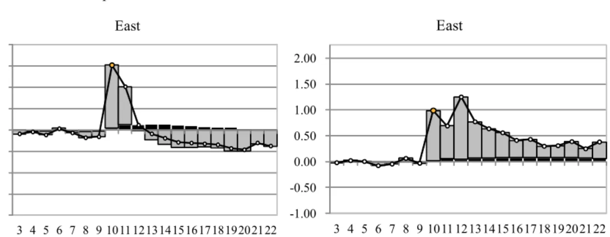
To explore changes in the intensive margin of bargain sales, we also compute the magnitude of bargain sales measured by the size of price reduction conditional on commodities sold at bargain sale prices. Figure 7 shows the magnitude of bargain sales in East . After the disaster, the size of price reduction in East dropped sharply from 14.4% to 13.3% (an 8% decline), but returned quickly to the pre-disaster level. In other words, immediately after the disaster, the frequency as well as magnitude of bargain sales declined sharply, raising within-store commodity prices.
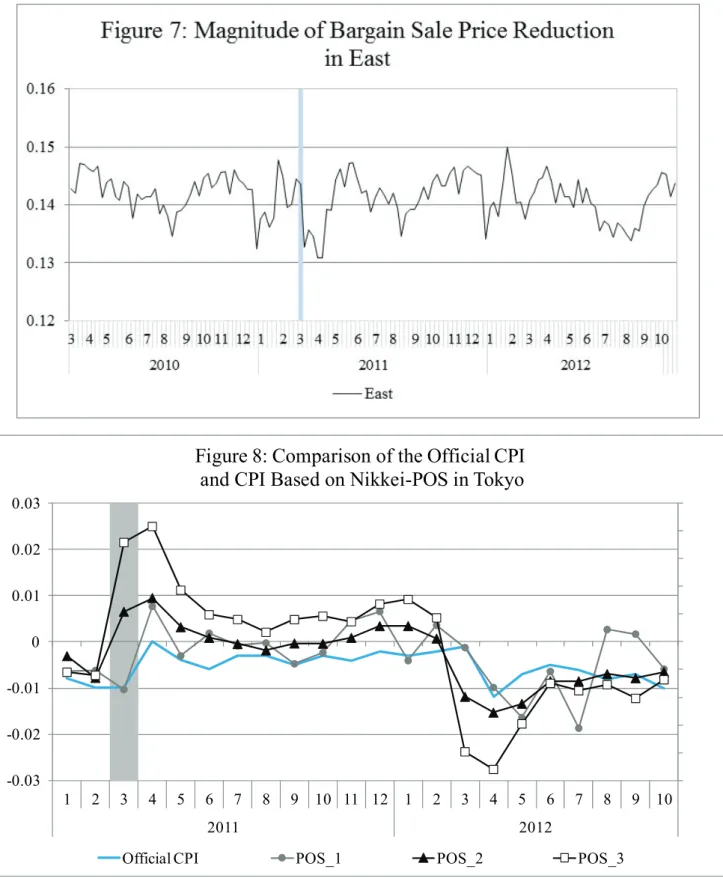
To assess the sources of the discrepancy between the official CPI and our CPI based on Nikkei-POS data more clearly, we focus on Tokyo and compare the rate of change in CPIs (for foods) from the same month in the previous year under varying definitions. In Figure 8, the solid line is the official CPI and the line labeled POS1 is a replication of the official CPI using Nikkei-POS data, in which we use the same (a) monthly survey dates, (b) Laspeyres weights, (c) a choice of commodities, and (d) price definition (excluding bargain sale prices) as in the official CPI. The official CPI and the POS1 do not entirely coincide due to the differences in their samples of retail stores. The line labeled POS2 is a CPI based on Nikkei-POS in which we use daily observations of all commodities and take the actual sales ratios as the weights, but exclude bargain sale prices. In contrast to POS1, POS2 is free from the Laspeyres bias and the lower substitution bias. Finally, the line labeled POS3 is the CPI based on Nikkei-POS that includes bargain sale prices. In other words, the difference between POS2 and POS3 represents the effects of bargain sales in increasing food prices after the disaster. According to
Figure 8, by incorporating information on bargain sales, the rate of change in CPI rose from
0.66% to 2.15% in March 2011. Roughly speaking, half of the increase in the within-store commodity prices can be attributed to changes in bargain sales.
In this section, we propose a new price index that can better capture the cost of living when consumers face severe commodity shortages. Note that all the price indices shown so far are standard indices based on within-store commodity prices, which essentially assumes that a set of commodities sold at any given store is stable over time. However, this assumption is hugely violated when excess demand meets supply constraints. As shown below, for certain categories, the number of commodities sold at retail stores fell dramatically after the disaster as they ran out of stock and recovered gradually with an inflow of new commodities that did not exist before the disaster. 11 Because the standard price index only follows within-store same-commodity prices over time, it fails to capture the effects of high commodity turnover on the cost of living.
We propose two alternative price indices. The first index is based on the average commodity price without distinguishing stores, which can capture commodity price changes arising from a shift of demand across store types as consumers search multiple stores to find the commodity when it is not available in their usual stores. The second index is based on “unit price” defined by the average price per weight, aggregating all commodities in the same category. This index can capture price changes arising from “higher substitution” in which consumers purchase a similar but more expensive item when the desired items are no longer available.
To compute the alternative price indices, we take advantage of INTAGE-POS data that cover a wide variety of retail stores, include virtually all commodities sold in each category, and contain volume information of each commodity (see Table 1). We focus on four categories of food for which the excess demand after the disaster was especially large: (1) cup noodle, (2) bottled water, (3) natto, and (4) yogurt. The demand for the first two goods surged after the disaster, as consumers tried to stockpile storable foods and beverages to prepare for heightened future uncertainty (Abe et al. 2013). In particular, due to the fear of radiation contamination of tap water, the demand for bottled water increased dramatically nationwide. By contrast, the excess demand for yogurt and natto was driven by supply-side constraints: the production of yogurt was curtailed due to electric power shortages while the supply of natto fell due to damages to production facilities.12
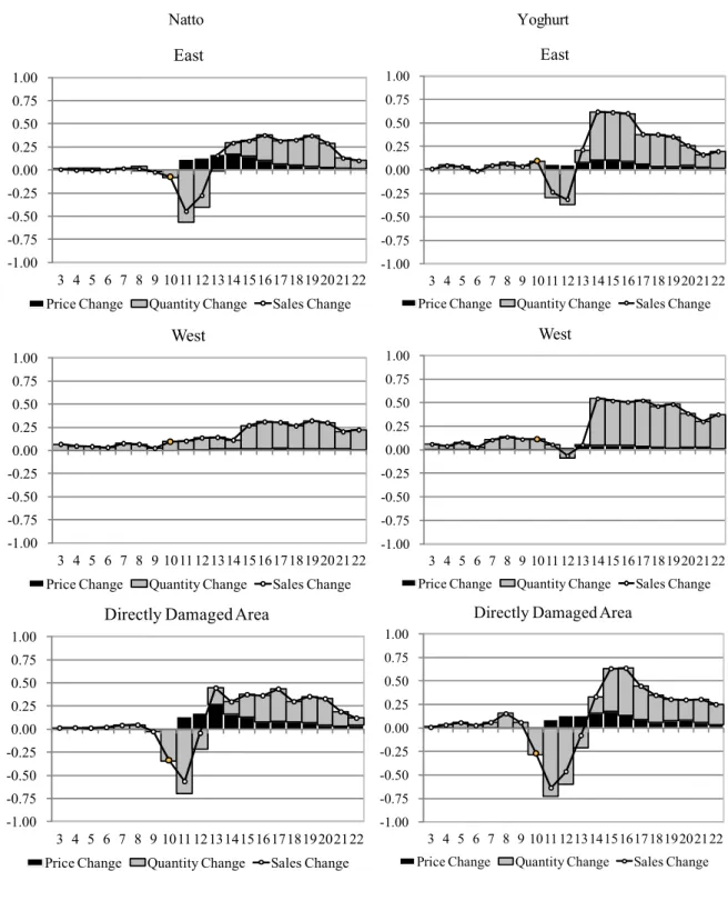
In Figures 9-1 and 9-2, we present the breakdown of the sales change into price and quantity changes for each category by geographical area. We take Week 2 as the base week and use the
11 Cavallo et al. (2013) also find that, at a leading online supermarket, the number of commodities
available for sale fell by 17% within 18 days after the disaster.
Fisher price index and the Fisher quantity index.13 Figure 9-1 shows that the sales of cup noodle increased by 75% in East and by 25% in West (but not in DAA for unknown reason) immediately after the disaster. It also shows that the sales of bottled water increased dramatically in all three areas and that the effect persisted for months in DAA and East. For both cup noodle and bottled water, price played little role in the observed sales increase. By contrast, Figure 9-2 shows the effects of supply shocks. The sales of natto and yogurt in DAA and East fell sharply after the disaster while West was unaffected, which implies that the supply shocks were local. For both natto and yogurt, an increase in price partly offset the sales decline.
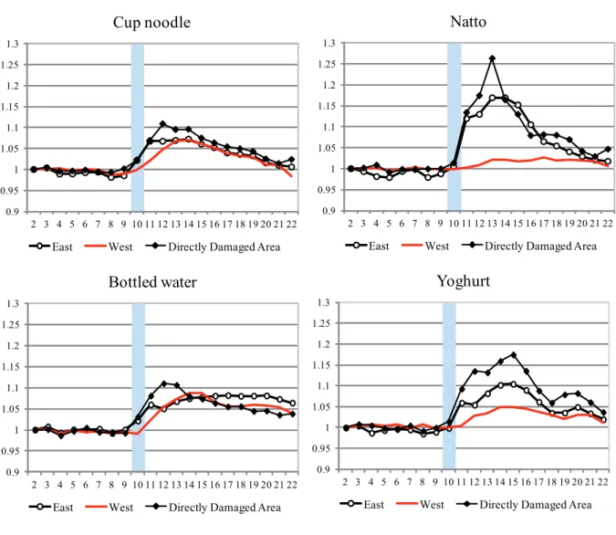
We first present the standard price index based on within-store same-commodity prices in INTAGE-POS data (including bargain sale prices). In Figure 10, we present the Fisher index for each category by geographic area, taking Week 2 as the base week. The standard indices reveal sizable price increase in DAA: the price rose by 10% for cup noodle, 9% for bottled water, 21% for natto, and 16% for yogurt. In East, the price increase was 5% for cup noodle, 8% for bottled water, 10% for natto, and 8% for yogurt. Although these are substantial changes, given the large excess demand induced by the disaster for these goods, we expect market clearing prices to be much higher. Moreover, our results from Nikkei-POS data suggest that part of these price increases were achieved through reductions in bargain sales rather than changes in regular prices. In other words, there is little evidence for price gorging in the case of the Great East Japan Earthquake.
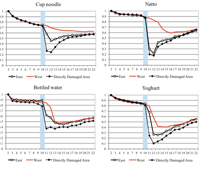
It is important to note that, to compute the standard price index, we must observe the price of the same commodity in the same store across weeks (i.e., in the base week and a subsequent week). However, a set of available commodities at a retail store changed greatly after the disaster as they ran out of stock. Figure 11 shows the number of observations (i.e., within-store same-commodity prices) used in computing the standard price index in Figure 10. To compare across areas, the number of observations in the base week is normalized to be one. Due to regular merchandize turnover, the number declined steadily even in normal times. However, in DAA and East, it fell dramatically from Week 10 to Week 11 and recovered gradually. For bottled water and yogurt, the impacts of the disaster are visible also in West. In other words, the standard price index during the weeks following the disaster is based on a small number of selected commodities that continued to be available at the same store. In this sense, the standard index is an inadequate measure for tracing the actual cost of living.
13 Note that the Fisher index passes the product test (i.e., total expenditure is equal to the product of quantity and price indexes), while the Paasche and Laspeyres indices do not (ILO 2005).
To capture the impacts of the disaster on the cost of living more precisely, we must take into account the effects of decline in commodity availability. We hypothesize that, when a desired commodity is unavailable in a usual store, consumers have three options: (1) to buy the desired commodity in a different store, (2) to buy a similar commodity that is available in the usual store, or (3) to buy nothing. In fact, according to Abe et al. (2011), the number of stores that consumers visited increased sharply in the week following the disaster in Tokyo. After the disaster, the market share of convenience stores increased substantially.14 These facts imply that consumers changed their store selection after the disaster.
To follow a shift of demand across stores, in Figure 12, we present the price index based on commodity prices without distinguishing stores. That is, we treat two goods with the same commodity code that are sold at different stores as identical goods. In DAA and East, for all categories, an increase in the price index based on across-store commodity prices was greater than that in the standard price index in Figure 10. The difference between the two indices was the largest for Natto, suggesting that a significant number of consumers in the disaster-stricken area and eastern Japan purchased the same brand of Natto at a higher price at a different store after the disaster.
To capture the effects of changing commodity compositions, in Figure 13 we present the price index based on unit prices (i.e., price per gram) without distinguishing commodities in the same category. In most cases, the increase in the price index based on unit prices was greater than that in the standard price index. The most striking results are obtained for bottled water in East and West: compared to an 8% increase in East and a 7% increase in West measured by the standard index, an increase in the unit price was 32% in East and 37% in East. This result is consistent with casual observations that in major supermarkets, two-litter bottled water was the first to run out of stock. As a result, demand shifted to smaller-sized bottled water or more expensive brands of bottled water. By sharp contrast, the unit price in DAA is volatile but shows a declining trend after the disaster. This may reflect the fact that a large quantity of bottled water was directed to the disaster-stricken area as part of rescue effort.
The merit of the index based on unit prices is that it captures the effect of new commodity inflows. In Figures 14, we show the breakdown of commodities in each week into “existing commodities” (commodities that were available also in Week 2) and “new commodities” (that became available in that week) in West, East and DAA. The number of commodities shown in
Figures 14-1, 14-2, and 14-3 coincides with the number of observations used to compute the
price index based on unit prices. The number of different cup noodles in West (Figure 14-1) shows a steady decline, which is mostly likely reflect the natural product turnover. It is clear that before the disaster, all three areas share the same trends for all the four categories. After the disaster, the number of commodities dropped for cup noodle, natto, and yoghurt in East and DDA. In the category of bottled water, the number of new commodities increased sharply after the disaster and continued to have a significant presence.
Finally, in Figures 15-1, 15-2, and 15-3, we compare the three price indices for each category in West, East and DDA. In West (Figure 15-1), except for bottled water, the standard price index follows the other two indices closely. In East (Figure 15-2), however, except for cup noodle, the standard price indices are significantly lower, underestimating the actual increase in the cost of living after the disaster. Three price indices show little difference in DDA (Figure 15-3), suggesting that the substitution between stores or products did not work strongly in DDA. It is also worth noting that the price index based on unit prices rose faster than the other two price indices, which indicates that consumers first responded to commodity shortages by purchasing whatever was available in the store.
5. Estimating the Price Elasticity of Demand
In the previous section, we proposed the two alternative price indices to better capture changes in the cost of living when consumers face severe commodity shortages. Our argument, however, is based on the assumptions that consumers care little about the difference in a store from which they purchase a commodity as well as the difference in quality associated with purchasing a similar but different commodity. To empirically assess the validity of these assumptions, we estimate two types of price elasticity using unit price: (1) price elasticity of demand between stores and (2) price elasticity of demand between commodities under the same category within the same store.
Let us assume an aggregate demand function with constant elasticity of substitution (CES). For between-store price elasticity, for each category, we estimate the following equation:
t t t
t t t
skt kt skt kt skt q p p T T q / )
ln( / )
ln( ,where
p
skt is the average unit price (i.e., price per gram) at store s in prefecture k in week t,p
kt is the average unit price in prefecture k in week t,q
skt is the average quantity at store sby unit in prefecture k in week t, and is a week indicator variable. For between-commodity price elasticity, we estimate the following equation:
t t t
t t t
iskt skt iskt skt iskt q p p T T q / )
ln( / )
ln( ,where and
p
iskt is the unit price of commodity i sold at store s in prefecture k in week t and is the quantity measured by unit of commodity i sold at store s in prefecture k in week t . For both equations, changes in the observed price elasticity across weeks can be captured by the coefficients . Our hypothesis is that observed price elasticity, which is normally negative, will increase (i.e., decrease in the absolute value) after the disaster, as consumers become less sensitive about the difference in stores or commodities in the face of commodity shortages. To presents the results of our regression analyses, in Figure 16 we plot estimated price elasticity (only if statistically significant at 1% level) by week. First, observe that, in normal times before the disaster, the elasticity is estimated to be negative and between -6 and -1 for all categories, which is generally consistent with preceding research (Hoch et al. 1995; Gordon et al. 2012). Second, in West, the elasticity changes relatively little before and after the disaster, which is also consistent with the fact that West was less affected by the disaster. Third, with respect to between-store elasticity, we observe a modest increase in the elasticity for bottled water in East and a large increase for natto and yogurt in DAA and East. Forth, with respect to between-commodity elasticity, we find a modest increase for natto and yoghurt in DAA and a large increase for cup noodle in DAA and East. For bottled water, whose unit prices increased sharply, we find no significant change in elasticity in East or West, however. Nevertheless, our estimation results are broadly in support of our hypothesis, indicating that, under severe commodity shortages, the same commodity sold at different stores, or even different commodities within the same category, became closer substitutes for consumers.6. Conclusion
In this paper, we analyze the impact of the Great East Japan Earthquake on commodity prices, taking advantage of large-scale high-frequency scanner data. We believe that this is the first study to empirically document the impact of natural disasters on prices using representative micro data. We show that the official CPI fails to capture the impact of the disaster on the cost of living, not only because it disregards the role of bargain sales in price adjustments, but also because it does not take into account changes in commodity availability after the disaster. Our alternative price indices suggest that a rise in the cost of living after the disaster in eastern
t
T
t
t
Japan, let alone the disaster-stricken area, was considerably greater than the standard price index would indicate.
Despite the large excess demand induced by the disaster, changes in within-store commodity prices were surprisingly modest even after including the effects of bargain sales reduction. This is in line with the findings of Cavallo et al. (2013) that large supermarkets changed their prices little after a major earthquake in Chile or Japan. These results indicate that price gouging was comparatively rare, casting some doubts on the popular view (e.g., Sandel 2009). In the case of the Great East Japan Earthquake, the excess demand was resolved, not through price adjustments, but mainly through quantity adjustments (see Abe et al. 2013 for more analysis). Why did not retailers increase their prices after the disaster? According to the customer market hypothesis proposed by Okun (1981), in a customer market where retailers set prices and consumers choose retailers, if search cost is high, consumers form long-term relations with retailers and become their “customers.” As retailers value customer relations, they refrain from increasing prices beyond what their customers regard as “fair” to maintain their reputation (Rotemberg 2011). It is difficult to test this hypothesis using our data, but if true, it implies that eliminating bargain sales was considered “fair,” while increasing regular prices was not. Another interesting question is why the disaster had a lasting effect in reducing the frequency of bargain sales especially in the Tokyo metropolitan area. One hypothesis is that, before the disaster, major retailers were engaging in an “excessive” price competition from their viewpoint and that the disaster became an opportunity for retailers to coordinate themselves to simultaneously reduce bargain sales and move to a new (and more cooperative) equilibrium. We leave further analysis of these questions to future work.
References
Abe, Naohito, Chiaki Moriguchi, and Noriko Inakura (2013). “The Great East Japan Earthquake and its Short-run Effects on Household Purchasing Behavior,” Hitotsubashi University Research Center for Price Dynamics Working Paper No. 2.
Abe, Naohito, and Akiyuki Tonogi, (2010) “Micro and Macro Price Dynamics in Daily Data,” Journal of Monetary Economics 57 (6): 716–728.
Abe, Naohito, Chiaki Moriguchi, and Noriko Inakura (2011). “The Impact of the Great East Japan Earthquake on Customer Relations and Supplier Relations in the Tokyo Metropolitan Area,” mimeo, Hitotsubashi University, August 2011 (in Japanese).
Broda, Christina, and John Romalis (2009). “The Welfare Implications of Rising Price Dispersion,” mimeo, Graduate School of Business, University of Chicago, July 2009. Cavallo, Alberto, Eduard Cavallo, and Roberto Rigobon (2013). “Prices and Supply
Disruptions during Natural Disasters,” NBER Working Paper No. 19474.
Davis, Cale Wren (2008). An Analysis of the Enactment of Anti-price Gouging Laws, Master’s Thesis, Department of Economics, Montana State University.
Gordon, Brett, Avi Goldfarb, and Yang Li (2013). “Does Price Elasticity Vary with Economic Growth? A Cross-Category Analysis,” Journal of Marketing Research, 50 (1): 4-23. Hoch, Stephen, Byung-Do Kim, Alan Montgomery, and Peter Rossi (1995). “The
Implementation Challenge of Pricing Decision Support Systems for Retail Managers,” Journal of Marketing Research 32, 1.
Hundbury, Jessie, Tsutomu Watanabe, and David. Weinstein, (2013). “How Much Do Official Price Indexes Tell Us about Inflation?” NBER Working Paper No. 19504.
Ivancic, Lorraine, Erwin Diewert, and Kevin Fox (2011). "“Scanner Data, Time Aggregation and the Construction of Price Indexes, ” Journal of Econometrics, 161 (1): 24-35.
International Labor Organization (2005). Consumer Price Index Manual: Theory And Practice.
Jorgenson, Dale (2006). “Price Measurement in the United States: A Decade After the Boskin Report,” Monthly Labor Review, May 2006, pp. 10-19.
Jorgenson, Dale, Michael J. Boskin, Ellen R. Dulberger, Robert J. Gordon, and Zvi Griliches (1996). Final Report of the Advisory Commission to Study the Consumer Price Index. Committee on Finance, United States Senate, One Hundred Fourth Congress, Second Session.
Ministry of Agriculture, Forestry and Fisheries (2012), Trend of Food, Agriculture, and Farm Villages.
Econometrica, 79 (4): 1139-1180.
Nakamura, Emi, and J. Steinsson (2008). “Five Facts about Prices: A Reevaluation of Menu Cost Models,” Quarterly Journal of Economics, 123 (4): 1415-1464.
Okun, Arthur (1981). Prices and Quantities: A Macroeconomic Analysis. Brookings Institution Press.
Rotemberg, Julio (2011). “Fair Pricing,” Journal of the European Economic Association, 9 (5): 952-981.
Sandel, Michael (2009). Justice: What’s the Right Thing to Do? Farrar Straus & Giroux. Shiratsuka, Shigenori, (1999). “Measurement Errors in the Japanese Consumer Price Index,”
Kinyu Kenkyu 14 (2): 1-45 (in Japanese).
Sudo, Nao, Kozo Ueda, and Kota Watanabe, (2014). “Micro Price Dynamics during Japan’s Lost Decades,” Asian Economic Policy Review, 9 (1): 44-64.
Table 1: Data Characteristics
Nikkei-POS INTAGE-POS Retail Price Survey
Data Frequency Daily Weekly Monthly
No. of Categories in Processed Foods 156 4 137
No. of Commodities Covered in:
Cup noodle 948 1,291 1
Bottled water 459 878 1~3
Natto 531 734 n/a
Yoghurt 807 966 1~3
All Categories 151,598 3,869 n/a
No. of Retail Stores by Area:
in Directly Damaged Area 8 171 n/a
in West 103 962 n/a
in East 55 495 n/a
Total 166 1,628 about 27,000
No. of Retail Stores by Store Type:
Supermarket (including GMS) 166 642 n/a
Convinience store 0 469 n/a
Drugstore 0 349 n/a
Discount liquor store 0 70 n/a
Home improvement retailer 0 98 n/a
Notes: Nikkei-POS and INTAGE-POS are provided by Nikkei Degital Media and INTAGE, respectively. The Retail Price Survey is the government survey that provides data to compute the official CPI. "n/a" means that information is not available.
Figure1: East, West, and Directly Damaged Area of Japan
Directly Damaged Area
East West
0
0.2
0.4
0.6
0.8
1
-0.03
-0.02
-0.01
0
0.01
0.02
0.03
0.04
0.05
2000 2001 2002 2003 2004 2005 2006 2007 2008 2009 2010 2011 2012 2013
Figure 2: Official CPI Change Rate
(All Goods and Services)
East
West
Directly Damaged Area
0
0.2
0.4
0.6
0.8
1
-0.03
-0.02
-0.01
0
0.01
0.02
0.03
0.04
0.05
2000 2001 2002 2003 2004 2005 2006 2007 2008 2009 2010 2011 2012 2013
Figure 3: Official CPI Change Rate (Foods)
-0.03 -0.025 -0.02 -0.015 -0.01 -0.005 0 0.005 0.01 0.015 1 2 3 4 5 6 7 8 9 10 11 12 1 2 3 4 5 6 7 8 9 10 11 12 1 2 3 4 5 6 7 8 9 10 11 12 2010 2011 2012
Figure 4-1: Decomposition of the Rate of Change
in the Official CPI (Foods) in Directly Damaged Area
Cereals Dairy products & eggs Oils, fats & seasonings
Cakes & candies Cooked food Beverages
Alcoholic beverages Total
-0.03 -0.025 -0.02 -0.015 -0.01 -0.005 0 0.005 0.01 0.015 1 2 3 4 5 6 7 8 9 10 11 12 1 2 3 4 5 6 7 8 9 10 11 12 1 2 3 4 5 6 7 8 9 10 11 12 2010 2011 2012
Figure 4-2: Decomposition of the Rate of Change
in the Official CPI (Foods) in East
Cereals Dairy products & eggs Oils, fats & seasonings
Cakes & candies Cooked food Beverages
-0.03 -0.025 -0.02 -0.015 -0.01 -0.005 0 0.005 0.01 0.015 1 2 3 4 5 6 7 8 9 10 11 12 1 2 3 4 5 6 7 8 9 10 11 12 1 2 3 4 5 6 7 8 9 10 11 12 2010 2011 2012
Figure 4-3: Decomposition of the Rate of Change
in the Official CPI (Foods) in West
Cereals Dairy products & eggs Oils, fats & seasonings
Cakes & candies Cooked food Beverages
Alcoholic beverages Total
0.98
0.99
1
1.01
1.02
1.03
1.04
2
3
4
5
6
7
8
9 10 11 12 13 14 15 16 17 18 19 20 21 22
week
Figure 5: CPI Based on Nikkei-POS (Foods)
0 0.1 0.2 0.3 0.4 0.5 0.6 0.7 0.8 0.9 1 -0.03 -0.02 -0.01 0 0.01 0.02 0.03 1 2 3 4 5 6 7 8 9 10 11 12 1 2 3 4 5 6 7 8 9 10 2011 2012
Figure 8: Comparison of the Official CPI
and CPI Based on Nikkei-POS in Tokyo
Figure 9-1: Decomposition of Sales Changes into Price and Quantity Changes (Demand Shocks)
Cup Noodle Bottled Water
-1.00 -0.75 -0.50 -0.25 0.00 0.25 0.50 0.75 1.00 3 4 5 6 7 8 9 1011 1213141516171819202122 East
Price Change Quantity Change Sales Change
-1.00 -0.75 -0.50 -0.25 0.00 0.25 0.50 0.75 1.00 3 4 5 6 7 8 9 1011 1213141516171819202122 West
Price Change Quantity Change Sales Change
-1.00 -0.75 -0.50 -0.25 0.00 0.25 0.50 0.75 1.00 3 4 5 6 7 8 9 1011 1213141516171819202122
Directly Damaged Area
Price Change Quantity Change Sales Change
-1.00 -0.50 0.00 0.50 1.00 1.50 2.00 3 4 5 6 7 8 9 1011 1213141516171819202122 East
Price Change Quantity Change Sales Change
-1.00 -0.50 0.00 0.50 1.00 1.50 2.00 3 4 5 6 7 8 9 1011 1213141516171819202122 West
Price Change Quantity Change Sales Change
-1.00 -0.50 0.00 0.50 1.00 1.50 2.00 3 4 5 6 7 8 9 1011 1213141516171819202122
Directly Damaged Area
Natto Yoghurt
Figure 9-2: Decomposition of Sales Changes into Price and Quantity Changes (Supply Shocks)
-1.00 -0.75 -0.50 -0.25 0.00 0.25 0.50 0.75 1.00 3 4 5 6 7 8 9 1011 1213141516171819202122 East
Price Change Quantity Change Sales Change
-1.00 -0.75 -0.50 -0.25 0.00 0.25 0.50 0.75 1.00 3 4 5 6 7 8 9 1011 1213141516171819202122 West
Price Change Quantity Change Sales Change
-1.00 -0.75 -0.50 -0.25 0.00 0.25 0.50 0.75 1.00 3 4 5 6 7 8 9 1011 1213141516171819202122
Directly Damaged Area
Price Change Quantity Change Sales Change
-1.00 -0.75 -0.50 -0.25 0.00 0.25 0.50 0.75 1.00 3 4 5 6 7 8 9 1011 1213141516171819202122 East
Price Change Quantity Change Sales Change
-1.00 -0.75 -0.50 -0.25 0.00 0.25 0.50 0.75 1.00 3 4 5 6 7 8 9 1011 1213141516171819202122 West
Price Change Quantity Change Sales Change
-1.00 -0.75 -0.50 -0.25 0.00 0.25 0.50 0.75 1.00 3 4 5 6 7 8 9 1011 1213141516171819202122
Directly Damaged Area
Figure 10: Standard Price Index Based on Within-Store Commodity Prices 0.9 0.95 1 1.05 1.1 1.15 1.2 1.25 1.3 2 3 4 5 6 7 8 9 10 11 12 13 14 15 16 17 18 19 20 21 22 Cup noodle
East West Directly Damaged Area
0.9 0.95 1 1.05 1.1 1.15 1.2 1.25 1.3 2 3 4 5 6 7 8 9 10 11 12 13 14 15 16 17 18 19 20 21 22 Natto
East West Directly Damaged Area
0.9 0.95 1 1.05 1.1 1.15 1.2 1.25 1.3 2 3 4 5 6 7 8 9 10 11 12 13 14 15 16 17 18 19 20 21 22 Yoghurt
East West Directly Damaged Area 0.9 0.95 1 1.05 1.1 1.15 1.2 1.25 1.3 2 3 4 5 6 7 8 9 10 11 12 13 14 15 16 17 18 19 20 21 22 Bottled water
Figure 11: Changes in the Number of Observations Used to Compute the Standard Price Index Based on Within-Store Commodity Prices
0 0.1 0.2 0.3 0.4 0.5 0.6 0.7 0.8 0.9 1 2 3 4 5 6 7 8 9 10 11 12 13 14 15 16 17 18 19 20 21 22 Cup noodle
East West Directly Damaged Area
0 0.1 0.2 0.3 0.4 0.5 0.6 0.7 0.8 0.9 1 2 3 4 5 6 7 8 9 10 11 12 13 14 15 16 17 18 19 20 21 22 Natto
East West Directly Damaged Area
0 0.1 0.2 0.3 0.4 0.5 0.6 0.7 0.8 0.9 1 2 3 4 5 6 7 8 9 10 11 12 13 14 15 16 17 18 19 20 21 22 Yoghurt
East West Directly Damaged Area 0 0.1 0.2 0.3 0.4 0.5 0.6 0.7 0.8 0.9 1 2 3 4 5 6 7 8 9 10 11 12 13 14 15 16 17 18 19 20 21 22 Bottled water
Figure 12: Price Index Based on Commodity Price without Distinguishing Stores 0.9 0.95 1 1.05 1.1 1.15 1.2 1.25 1.3 2 3 4 5 6 7 8 9 10 11 12 13 14 15 16 17 18 19 20 21 22 Cup noodle
East West Directly Damaged Area
0.9 0.95 1 1.05 1.1 1.15 1.2 1.25 1.3 2 3 4 5 6 7 8 9 10 11 12 13 14 15 16 17 18 19 20 21 22 Natto
East West Directly Damaged Area
0.9 0.95 1 1.05 1.1 1.15 1.2 1.25 1.3 2 3 4 5 6 7 8 9 10 11 12 13 14 15 16 17 18 19 20 21 22 Yoghurt
East West Directly Damaged Area 0.9 0.95 1 1.05 1.1 1.15 1.2 1.25 1.3 2 3 4 5 6 7 8 9 10 11 12 13 14 15 16 17 18 19 20 21 22 Bottled water
Figure 13: Price Index Based on Unit Prices without Distinguishing Commodities 0.8 0.9 1 1.1 1.2 1.3 1.4 2 3 4 5 6 7 8 9 10 11 12 13 14 15 16 17 18 19 20 21 22 Cup noodle
East West Directly Damaged Area
0.8 0.9 1 1.1 1.2 1.3 1.4 2 3 4 5 6 7 8 9 10 11 12 13 14 15 16 17 18 19 20 21 22 Natto
East West Directly Damaged Area
0.8 0.9 1 1.1 1.2 1.3 1.4 2 3 4 5 6 7 8 9 10 11 12 13 14 15 16 17 18 19 20 21 22 Yoghurt
East West Directly Damaged Area 0.8 0.9 1 1.1 1.2 1.3 1.4 2 3 4 5 6 7 8 9 10 11 12 13 14 15 16 17 18 19 20 21 22 Bottled water
Figure 14-1: Composition of the Commodities Used to Compute the Price Index Based on Unit Prices (West)
0 100 200 300 400 500 600 700 800 900 2 3 4 5 6 7 8 9 10 11 12 13 14 15 16 17 18 19 20 21 22 Cup noodle
Commodities in week 2 New Commodities
0 50 100 150 200 250 300 350 400 2 3 4 5 6 7 8 9 10 11 12 13 14 15 16 17 18 19 20 21 22 Natto
Commodities in week 2 New Commodities
0 50 100 150 200 250 300 350 400 450 500 2 3 4 5 6 7 8 9 10 11 12 13 14 15 16 17 18 19 20 21 22 Bottled water
Commodities in week 2 New Commodities
0 100 200 300 400 500 600 2 3 4 5 6 7 8 9 10 11 12 13 14 15 16 17 18 19 20 21 22 Yoghurt
Figure 14-2: Composition of the Commodities Used to Compute the Price Index Based on Unit Prices (East)
0 100 200 300 400 500 600 700 800 900 2 3 4 5 6 7 8 9 10 11 12 13 14 15 16 17 18 19 20 21 22 Cup noodle
Commodities in week 2 New Commodities
0 50 100 150 200 250 300 2 3 4 5 6 7 8 9 10 11 12 13 14 15 16 17 18 19 20 21 22 Natto
Commodities in week 2 New Commodities
0 50 100 150 200 250 300 350 400 450 2 3 4 5 6 7 8 9 10 11 12 13 14 15 16 17 18 19 20 21 22 Bottled water
Commodities in week 2 New Commodities
0 50 100 150 200 250 300 350 400 450 500 2 3 4 5 6 7 8 9 10 11 12 13 14 15 16 17 18 19 20 21 22 Yoghurt
Figure 14-3: Composition of the Commodities Used to Compute the Price Index Based on Unit Prices (Directly Damaged Area)
0 100 200 300 400 500 600 700 800 2 3 4 5 6 7 8 9 10 11 12 13 14 15 16 17 18 19 20 21 22 Cup noodle
Commodities in week 2 New Commodities
0 50 100 150 200 250 2 3 4 5 6 7 8 9 10 11 12 13 14 15 16 17 18 19 20 21 22 Natto
Commodities in week 2 New Commodities
0 50 100 150 200 250 300 2 3 4 5 6 7 8 9 10 11 12 13 14 15 16 17 18 19 20 21 22 Bottled water
Commodities in week 2 New Commodities
0 50 100 150 200 250 300 350 400 2 3 4 5 6 7 8 9 10 11 12 13 14 15 16 17 18 19 20 21 22 Yoghurt
Figure 15-1: Comparing the Three Price Indices (West) 0.95 1 1.05 1.1 1.15 1.2 1.25 1.3 1.35 2 3 4 5 6 7 8 9 10 11 12 13 14 15 16 17 18 19 20 21 22 Cup noodle
Within-store commodity price
Commodity price without distinguishing stores Unit price without distinguishing commodities
0.9 1 1.1 1.2 1.3 1.4 2 3 4 5 6 7 8 9 10 11 12 13 14 15 16 17 18 19 20 21 22 Bottled water
Within-store commodity price
Commodity price without distinguishing stores Unit price without distinguishing commodities
0.95 1 1.05 1.1 1.15 1.2 1.25 1.3 1.35 2 3 4 5 6 7 8 9 10 11 12 13 14 15 16 17 18 19 20 21 22 Natto
Within-store commodity price
Commodity price without distinguishing stores Unit price without distinguishing commodities
0.95 1 1.05 1.1 1.15 1.2 1.25 1.3 1.35 2 3 4 5 6 7 8 9 10 11 12 13 14 15 16 17 18 19 20 21 22 Yoghurt
Within-store commodity price
Commodity price without distinguishing stores Unit price without distinguishing commodities
Figure 15-2: Comparing the Three Price Indices (East) 0.95 1 1.05 1.1 1.15 1.2 1.25 1.3 1.35 2 3 4 5 6 7 8 9 10 11 12 13 14 15 16 17 18 19 20 21 22 Cup noodle
Within-store commodity price
Commodity price without distinguishing stores Unit price without distinguishing commodities
0.95 1 1.05 1.1 1.15 1.2 1.25 1.3 1.35 2 3 4 5 6 7 8 9 10 11 12 13 14 15 16 17 18 19 20 21 22 Bottled water
Within-store commodity price
Commodity price without distinguishing stores Unit price without distinguishing commodities
0.95 1 1.05 1.1 1.15 1.2 1.25 1.3 1.35 2 3 4 5 6 7 8 9 10 11 12 13 14 15 16 17 18 19 20 21 22 Natto
Within-store commodity price
Commodity price without distinguishing stores Unit price without distinguishing commodities
0.95 1 1.05 1.1 1.15 1.2 1.25 1.3 1.35 2 3 4 5 6 7 8 9 10 11 12 13 14 15 16 17 18 19 20 21 22 Yoghurt
Within-store commodity price
Commodity price without distinguishing stores Unit price without distinguishing commodities
Figure 15-3: Comparing the Three Price Indices (Directly Damaged Area) 0.95 1 1.05 1.1 1.15 1.2 1.25 1.3 1.35 2 3 4 5 6 7 8 9 10 11 12 13 14 15 16 17 18 19 20 21 22 Cup noodle
Within-store commodity price
Commodity price without distinguishing stores Unit price without distinguishing commodities
0.8 0.9 1 1.1 1.2 1.3 2 3 4 5 6 7 8 9 10 11 12 13 14 15 16 17 18 19 20 21 22 Bottled water
Within-store commodity price
Commodity price without distinguishing stores Unit price without distinguishing commodities
0.95 1 1.05 1.1 1.15 1.2 1.25 1.3 1.35 2 3 4 5 6 7 8 9 10 11 12 13 14 15 16 17 18 19 20 21 22 Natto
Within-store commodity price
Commodity price without distinguishing stores Unit price without distinguishing commodities
0.95 1 1.05 1.1 1.15 1.2 1.25 1.3 1.35 2 3 4 5 6 7 8 9 10 11 12 13 14 15 16 17 18 19 20 21 22 Yoghurt
Within-store commodity price
Commodity price without distinguishing stores Unit price without distinguishing commodities
Table 2: Maximum Price Increase in the Three Price Indices DAA Within-store commodity prices Across-store commodity prices Unit prices Cup noodle 10.3% 10.9% 10.6% Bottled water 9.3% 11.0% 8.4% Natto 21.2% 26.3% 20.1% Yogurt 16.2% 17.5% 18.7% East Within-store commodity prices Across-store commodity prices Unit prices Cup noodle 5.0% 7.2% 10.8% Bottled Water 8.1% 8.2% 34.1% Natto 10.4% 16.9% 18.3% Yogurt 8.6% 10.5% 18.0% West Within-store commodity prices Across-store commodity prices Unit prices Cup noodle 5.8% 7.1% 8.4% Bottled Water 6.5% 8.7% 38.5% Natto 1.9% 2.7% 2.4% Yogurt 4.6% 4.9% 2.6%
Figure 16: Changes in Price Elasticity of Demand
Cup noodle 0 0.1 0.2 0.3 0.4 0.5 0.6 0.7 0.8 0.9 1 -4 -3.5 -3 -2.5 -2 -1.5 -1 -0.5 0 5 6 7 8 9 10 11 12 13 14 15 16 17 18 19 20 21 22 (1) Between StoresEast West Directly Damaged Area
0 0.1 0.2 0.3 0.4 0.5 0.6 0.7 0.8 0.9 1 -1.6 -1.4 -1.2 -1 -0.8 -0.6 -0.4 -0.2 0 5 6 7 8 9 10 11 12 13 14 15 16 17 18 19 20 21 22 (2) Between Commodities
East West Directly Damaged Area
Bottled water 0 0.1 0.2 0.3 0.4 0.5 0.6 0.7 0.8 0.9 1 -3 -2.5 -2 -1.5 -1 -0.5 0 5 6 7 8 9 10 11 12 13 14 15 16 17 18 19 20 21 22 (1) Between Stores
East West Directly Damaged Area
0 0.1 0.2 0.3 0.4 0.5 0.6 0.7 0.8 0.9 1 -2.5 -2 -1.5 -1 -0.5 0 5 6 7 8 9 10 11 12 13 14 15 16 17 18 19 20 21 22 (2) Between Commodities
East West Directly Damaged Area
Natto 0 0.1 0.2 0.3 0.4 0.5 0.6 0.7 0.8 0.9 1 -6 -5 -4 -3 -2 -1 0 1 2 5 6 7 8 9 10 11 12 13 14 15 16 17 18 19 20 21 22 (1) Between Stores
East West Directly Damaged Area
0 0.1 0.2 0.3 0.4 0.5 0.6 0.7 0.8 0.9 1 -3 -2.5 -2 -1.5 -1 -0.5 0 5 6 7 8 9 10 11 12 13 14 15 16 17 18 19 20 21 22 (2) Between Commodities
East West Directly Damaged Area
Yoghurt 0 0.1 0.2 0.3 0.4 0.5 0.6 0.7 0.8 0.9 1 -6 -5 -4 -3 -2 -1 0 5 6 7 8 9 10 11 12 13 14 15 16 17 18 19 20 21 22 (1) Between Stores
East West Directly Damaged Area
0 0.1 0.2 0.3 0.4 0.5 0.6 0.7 0.8 0.9 1 -2.5 -2 -1.5 -1 -0.5 0 5 6 7 8 9 10 11 12 13 14 15 16 17 18 19 20 21 22 (2) Between Commodities