先史ヨーロッパにおける農耕文化圏拡大に関する数理モデル考察

Kagamiyama 1-3-1, Higashi-hiroshima,

724

Hiroshima,JAPAN

先史ヨーロッパにおける農耕文化圏拡大に関する数理モデル考察

広島大学理学部 瀬野裕美

Amathematical model ofthedispersal of colonies produced bythe stochasticmigrationprocess

dependingonthe totalpopulation of thegroupis considered. The expected velocity of the spatial expanding ofthe settlementrangeofcolonies is analyzed,utilizing the fractal concept appliedto

the pattern of spatialdistributionofcolonies. The model isused toconsiderthespreadmg phenomenon ofearly farIninnginEurope, with the data of neolithic sites with C-14 dates.

INTRODUCTION

Theexpandingof thedistribution

area

of

some

animalshasbeen theoretically studiedbymathematical models. As for patterns of spatialdistributionand the expanding velocity,

some

diffusion models have been appliedtounderstand such

phenomena (AmmermanandCavalli-Sforza, 1984;Martin, 1973; Mosimannand

Martin, 1975; Okubo, 1980; Skellam, 1951). Those phenomenaconsidered by

diffusion models should have such

a

characteristic that the spatial distribution

can

be regarded

as

continuousin

space.

However,for such phenomena that the spatial distribution essentiallyconsistsof

a

number of spatially disconnected islands,that

is, colonies, theanalysis bythediffusion model has torequire

some

additional

assumptions,and should be regarded

as an

approximate approach.

Inthis

paper,

fortheexpanding of settlement

area

consistingof

a

number

ofcoloniesispresented,

a

mathematical model ofstochasticmigration

processes

is

proposed (Bartlett, 1978). Inorderto givetherelation between thenumber of colonies andthesettlement

area

occupied bythem, the fractalconceptis

introduced. Analyzing themodel,

we

derive the expected velocity of the expanding of settlement

area.

The modelis appliedtothedata of neolithic sites

with C-14dates, which

was

usedby Ammerman and Cavalli-Sforza(1984)in

order todiscuss thespreading phenomenon ofearly farming in Europe. The

expanding velocity of the settlement

area

offarming colonies is estimated by

our

COLONY PRODUCTION

Free Migration Process: A

new

colony is produced by

a

random migration

process

in theexisting

group

ofcolonies,with

a

constantmigration probability

independentof

any

otherparameter(Bartlett, 1978). That is,theprobabilityofthe production of

a new

colony isconstant,independent of

any

other parameters.

Now,itisassumed thatthe colony doesnotbecomeextinct

once

itis produced. Under theseassumptions, the followingmodel

can

be defined:

$\frac{d}{dt}P(k, t)=-\lambda P(k, t)+XP(k-1, t)$ (1)

$P(k, 0)=6_{k)}$,

where

$\lambda dr$

.

theprobabilityofproduction of

new

colony during $(t, t+dt)$

$P(k, t)$

:

theprobability of$k$colony productions during time-period _{$(0, t)$}

.

$6_{k0}$isthe kronecker’s delta

so

that the initialcondition

means

thatthereis

no

colony production at$t=0$

.

This colony production system results in the Poisson

probability distribution $P(k, t)$

:

$P(k, t)= ff^{\lambda t}\frac{(\lambda t)^{k}}{k!}$ (2)

Theexpectednumberofcolonies produced during $(0, t)$ is

$k h=\sum_{k=0}kP(k, t)=\lambda t$, (3)

and theexpectedtimeof the k-th colony production is

$rangFig$

.el.byScheemiaz

線

crfietni

躍註灘欝露盤

ent

explanation,seetext.

Size-dependent Migration Process: The migration probability is assumedto

depend

on

thetotal population of the

group

(Fig. 1). This

means

thatthecolony production isenhanced

more

and

more

as

the totalpopulation becomes larger. Under thisassumption,

we

consider the followingmodel:

$\frac{d}{dt}P(k, t)=-\}\iota N(t)P(k, t)+\mu N(t)P(k-1, t)$ (5)

$P(k, 0)=$ _り,

where

$N(t)$

:

the totalpopulation sizeof the

group

of coloniesattime$t$

$\mu N(t)dt$; theprobabilityof production of

new

colony during time-period$(t, t+dt)$

.

This colony production system in time$t$results in thePoissonprobability

distribution$P(k, 7)$ in time$T$

:

$P(k, T)=e-\downarrow 1T_{\frac{(\mu\tau Y}{k!}}$ (6)

where the time$T$is

now

transformed from time$t$

as

follows:

$T=T(t)= \int_{0^{t}}N(\tau X1\tau.$ (7)

Since

a

colony does notbecomeextinct after

its

production,

we

find that $Tarrow\infty$

as

$tarrow\infty$

.

Theaboveresultintime$T$coincides with that for thepreviouscase, that

is, for the

case

offreemigration

process.

Therefore, theexpected numberof colonies produced during $(0, t)$ is

$\Psi\lambda=\sum_{k=0}^{\infty}kP(k, T)=[\iota T=\mu\int_{0}^{t}N(\tau)d\tau$, (8)

and the expectedtime of the k-th colony production is

$t^{\tau}k=\int_{0}^{\infty}\tau P(k-1, \tau)\}\downarrow d\tau=\frac{k}{\downarrow 1}$

.

(9)

Then, the expectedtimein$t$

can

beobtained through the following relation:

$t k=T^{-1}(\{\phi=T^{-1}(\frac{k}{\mu})$

(10)

where$T^{-1}$ denotes theinverse function of_$T=T(t)$

.

EXPANSION OF SETTLEMENTAREA

Next,

we

consider the settlement

area

ofthe

group

of colonies. The settlement

area

attime$t$correspondstothe

area

thathas been occupiedby thoseexisting

coloniesatthetime. We characterize thesettlement

range

bytheminimal

diameter,

say

$R$, which

can

include all existing colonies.

In the

case

when thesettlement

area

expands in

every

direction with the

same

probability,the shape of thesettlement

area can

beapproximated by thedisc,

andtherefore, when the spheric nature of the earth

can

benegligibleandbe

approximated well bythe plane, the

range

$R$approximatelyhas thefollowing

relation withthetotal number of colonies $M;M\propto R^{2}$

.

_However, since_the expanding of the settlement

area

is constrained by geography,climate, cultural

factors, etc.,theshape is in generalpossibly inhomogeneous in direction. Itis

likely that the shape has

a

_fractal

nature (fortheconcept of’ffactal’, see, for

instance, Mandelbrot, 1982). To deal withsuch cases,

we

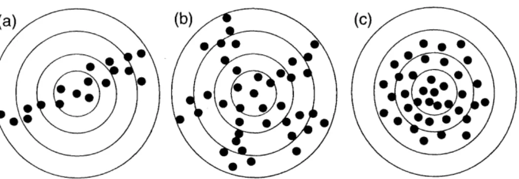
assume

thegeneralized

Fig.2. Illustrative explanation of therelation of the fractal dimension$d$tothe spatial pattern of colonydistribution. Each black disc shows each colony. (a)$d\sim 1;(b)1<d<2;(c)d\sim 2$.

$M\propto R^{d}$ _{$(1 \leq d\leq 2)$, (11)}

wherethe

power

$d$charactenizes the spatial pattern of the settlement

area

occupied

by colonies(Fig. 2). Itiscalled cluster dimension

or mass

dimension,whichis

one

_offractal

dimensions. When$d\sim 2$, the spatialdistribution of colonies

can

be approximated by

a

disc. When$d\sim 1$, thedistributionis

one

dimensional, that is, the colonies

are

arrayed

on

a

curve.

Forexample, the latter

case

may

correspond

tothe

case

whenthecolonies

are

located along

a

river.

Through therelation (11),

we

can

consider thevelocity of the expanding of the settlement

range.

That is, thevelocity $V$is given by

$V= \frac{dR}{dt}\propto\frac{d}{dt}(M^{1/d})=\frac{1}{d}\cdot M^{(1-yd}\cdot\frac{dM}{dt}$

.

(12)

Sincetheexpectedtota1 numberof coloniesattime$t$is given by$kh$, theexpected

range

of thesettlement

area

isproportionalto$k\Psi^{d}$

.

Therefore,

we

consider the

expected velocity $V_{t}$ attime$t$

as

follows:

$\ovalbox{\tt\small REJECT}\propto\frac{1}{d}\cdot\phi h^{(1-dy_{d}\ovalbox{\tt\small REJECT}}d_{dt}$

.

(13)

Forthe

case

ofthefreemigration

process,

the expected velocityis

$\overline{V_{t}}\propto\frac{\lambda^{1/d}}{d}t^{(1-\nu d}$ , (14)

$\overline{V_{t}}\propto\frac{\mu^{1/d}}{d}\cdot N(t)$

.

$[ \int_{0^{t}}N(\tau)d\tau]^{1-dy_{d}}$

.

(15)

LOGISTICGROWTH OFPOPULATION

As

an

exampleof the size-dependentmigration

process,

we

deal withthe

case

whenthetotal population size of the

group

of colonies

grows

in the logistic

manner

(Fig. $3(a)$):

$N(t)=N(0) \cdot\{(1-\frac{N(0)}{K})e^{-}’+\frac{N(0)}{K}\backslash /^{-1}$

, (16)

where$\epsilon$ isthe intninsicgrowthrateofthepopulation and$K$isthecarrying

capacityforthetotal population ofthe

group.

In thiscase,

some

fundamental calculations show

(17) $k)_{l}= \frac{\mu}{\epsilon}\cdot K\cdot\ln\{\frac{N(0)}{K}\cdot(\not\in-1)+1\}$

$\#k=\frac{1}{\epsilon}\ln\{\frac{K}{N(0)}\cdot(e^{(\epsilon 1\downarrow\downarrow)k/\kappa_{-1)+}}1\}.$

(18)

Generic feature oftheseexpectedvaluesis shownin Fig. 3(b) and Fig. 3(c). The

time interval betweenthe nearest twocolony productions is givenby

$\#k+1-\#k=_{\frac{1}{\epsilon}}\ln\{\frac{e^{\epsilon/(\mathscr{O}}+\frac{N(0)}{K}(1-\frac{N(0)}{K})\cdot e^{-(\epsilon 1\downarrow\downarrow)k/K}}{1+\frac{N(0)}{K}(1-\frac{N(0)}{K})\cdot e^{-(\epsilon 1\downarrow\iota)k/K}}\{$

.

(19)

Thisvalue tendsto

a

constant $l/pK$

as

$karrow\infty$, which

means

thatthecolony

productionisexpectedto

occur

periodically. In addition, from (17) and (18), for sufficiently large$t$and sufficiently large$k$,

(a)Typica1time-development of logistic populationgrowth;(b)Typical Typical

lk

$\cdot$

$\phi h^{\sim}t$ (20)

$\#k^{\sim k}$

.

(21)

Thatis, these expected valuesincrease linearly in

a

sufficiently

grown group,

whichis the

same as

for the

case

of the freemigration

process.

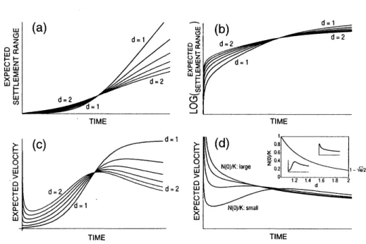
In this case, the expanding

way

of settlement

range

essentiallydepends

on

thefractal dimension$d$(Fig. _$4(a,$$b)$). Theexpected velocity of expanding of settlement

range

isexpressed

as

follows:

$\overline{V_{t}}\propto\frac{\epsilon}{d}(\frac{\mu K}{\epsilon})^{1/d}\frac{N(0)}{K}\cdot\frac{e^{\sigma}}{\{\frac{N(0)}{K}\cdot(\theta-1)_{/}+1^{\backslash }[\ln\{\frac{N(0)}{K}\cdot(\theta-1)+1^{1_{(}}]^{1-11d}}$

.

(22)

For $1<d\leq 2$_{, this}expected velocity decreases_to

zero

_at

a

_{sufficiently large}time

(Fig.$4(c,$$d)$). This

means

that, for

a

sufficiently

grown group,

thevelocity of the

expanding of settlement

range

is

very

small,whilethe number of colonies continuously increases; thatis, the

new

coloniestend to beproduced within the vacant

areas

among

the pre-settledcolonies. Ontheotherhand, the

time-development oftheexpectedvelocity intheearlier period depends

on

theinitial

population sizeofthe

group

(Fig. $4(d)$). Inthe

case

when the initial populationis

sufficiently large, the expectedvelocity monotonically decreases in time, while in the

case

when itis small, theexpectedvelocity increasesin theearlierperiod and decreases after peaking. Analytically,if thefollowing conditionis satisfied, the former

case

occurs, and otherwisethelatter(Fig. $4(d)$):

Fig. 4. Inthesize-dependent immigrationprocessmodel for the logistic population growth, thecontnibution ofthefmctal dimension$d$and the initialpopulationsize

$N(O)/K$to: $(a, b)$thetime-development of the expected settlementrange$R$,thatis,

$kt^{/d}$

:

$(c, d)$thetime-development of the expected velocity

17.

For(c),$N(O)/K=$ 0.1,and for(d),$d=1.5$. _{The graph shape of the}expected velocity $\overline{V_{t}}$

depends on$d$ and$N(O)/K$asshown totallyinthefigure attachedto(d).

This condition

can

beeasily derived by examining thesignof the t-derivative of

(22).

Intheperiod when thepopulation size$N(t)$ is sufficientlysmall, the

population growth

can

be well-approximated by exponential growth. Inthis

period,the

same

argument

as

abovegives theapproximateresults

on

thebehavior ofcolonydispersal

as

follows:

$N(t)\approx N(0ffl$ (24)

$k h^{\approx}\frac{\mu}{\epsilon}N(0X\not\in-1)$ (25)

$\#k^{\approx}\frac{1}{\epsilon}\ln(\frac{\epsilon/\mu}{N(0)}k+1)$ (26)

$\#k+1-\#k^{\approx}\frac{1}{\epsilon}\ln(\frac{N(0)+\epsilon(k+1y\mu}{N(0)+\epsilon H\mu})$ (27)

longitude

Fig. 5. 106neolithic European sitesinthegeographiccoordinates,used by AmmermanandCavalli-Sforza(1984). The blacksquareindicates the oldestsite,

Aswad(9690B.C.,C-14date). Black discs are forthosesites before5800B.C.

(C-14date),and whiteonesforthose after5800B.C.

In this case, theexpectedvelocity increasesexponentially while the number of coloniesgrows exponentially.

SPREAD OFEARLYFARMING INEUROPE

Ammerman and Cavalli-Sforza(1984) calculated theisochron

map

of the spread of early farming inEurope from the data of

106

neolithic European sites with

C-14 dates(9690 B.C.

-4160

B.C.). Thecomputer-generatedisochron

map

gives

the impressionthatearly farming might have spread in

a

spatiallycontinuous

manner

in Europe. This is

an

approximationtothe spatial spread through the analogy of diffusionprocess. However,in contrast to thespatial spread ofvarious

species ofanimals, insects, and plants, the spatial spread of

a group

of humans frequentlyinvolves theproduction spatially disconnectedunits,thatis,colonies. The spatial distribution expandsessentially by

a

seriesof productions of

new

colonies. The spread of early farming in Europe, dealt with by Ammerman and Cavalli-Sforza(1984),

_can

be regarded

as

such

a

case.

Inthis section,

we

apply

our

mathematical model described aboveto the

data and estimate the parameters of the model totrytodiscuss

some

features of the spread ofearly farming in Europe.

As forthe

way

ofpopulation growth,

we

assume

theexponential

one

given

by (24). This is appropriate inthe

case

when the population growthdoes not

time

Fig.6. Time-development of the number of neolithic sites,which iscumulatedafter the oldestsite,Aswad(9690B.C.,C-14date). Timeaxisshowsthe C-14 date passed$aRer$9690B.C. All 106neolithic sitesareplotted forthedata of Ammerman

andCavali-Sforza(1984). $k1$ curveforthe exponential growthinthe

size-dependentmigrationprocessmodelisoverlaid,fitto76data of neolithicsites

$($before5800B.C.(C-14 date). $\mu N(O)/\epsilon=3.352$and$\epsilon=8.233x10^{-4}$in

(25).

Fig.

5

showsthe

106

neolithic European sites in the geographic coordinatesusedbyAmmerman andCavalli-Sforza(1984). Theirspatial

distribution

seems

toshow inhomogeneity in direction. Beginning with the oldest

site, Aswad(9690 B.C.;

33.

$36N,$ $36.30E$),

we

countthecumulative number of

colonies inorderofdescending C-14 date

as

shownin Fig.

6.

Plotsin the figure indicate that thecontinuityof the time-development of the number of colonies

seems

tobreakataround

3800 years

after Aswad (i.e.,around

5800

B.C.). Thus,

we use

only the

76

data before

5800

B.C.,

up

tothesite Reichtett(5940B.C.;

48.

$6N,$$7.75E$_).

SinceFig.

6

can

be regarded

as

coIrespondingtothe time-developmentof

$k)_{t}$ ,

we

trytofit$\ell_{\{}$

}

$i$ given by (25)to the data. Theresultis overlaid in Fig.

6.

The

estimated parameters result in$\mu N(O)/\epsilon=3.572;\epsilon=8.233^{x}10^{-4}$

.

Next,

we

try toestimate the ffactal dimension$d$thatcharacterizes the

patternof spatial distribution. From(11), the

range

$R$ of thesettlement

area

and

the number$M$of colonieswithin ithavetherelation: $\log M=d\cdot\log R+const$

.

Therefore,

we

can

estimate$d$fromthe slope ofthe linefitto theplots of log$M$

against$\log R$

.

Thediameter

can

be calculated from the data of the locations of

neolithicsites (Fig. 7). We

use

thegyration-radius methodtoestimatethe

parameter$d$(as forthe method, see, forinstance, Mandelbrot, 1982). All

76

sites

before

5800

B.C.

are

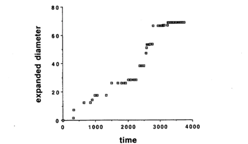
considered. The numberofsitesdistributed withinthedisc centeredat theoldest site, Aswad,iscounted. For disc radius large enoughto

time

Fig.7. Expandeddiameterof thesettlementrange. Time axis shows the C-14 date passed after9690B.C.

$\underline{\frac{\wedge oc\wedge}{*\vee oooo}}$

log(r) Iog(expanded diameter)

Fig. 8. (a)Number ofsiteswithin thedistance$r$from the oldestsite, Aswad,in log-log coordinates. For the distance$r$thatcontainsmorethan 10sites,plots fit wellto theline with the slope 1.671. (b)Relation between the expanded diameter of settlementareaand the number of coloniesinlog-log coordinates. The overlaidline

indicates theslope 1.671. Theunitof measured distance is conventionallyselected.

radius

can

befittedwellby

a

straight line with slope 1.671,

as

estimatedby the least-square method(Fig. $8(a)$). Hence,the spatialdistribution ofneolithicsitesis

estimated to have thecharacteristicfractal dimension$d=1.671$

.

Since the

diameter and the number of neolithic sites

are

time-dependent,it islikely that the

paIameter$d$might change in time in the periodconsidered

now.

However,

as

Fig.

8(b) shows,the time-dependent relation between the expanded diameter and the

number of colonies in log-logcoordinates, theestimated$d=1.671$

even

holds well. Therefore,

we

dealwith$d$

as

time-independent constant:$d=1.671$

.

From (28) withthese estimated parameters, the time-development ofthe

expected velocity of the expanding ofsettlementrange

can

bedrawn,resulting in Fig. 9(a). It

can

be

seen

that the velocity isrelatively small in the first century after Aswadandthenincreasesexponentially. In Fig. 9(b), the

same

expected

time #colony

Fig. 9. Time-development of the expectedvelocity(28)of the expanding of the settlementarea,for$\mu N(O)/\epsilon=3.352;\epsilon=8.233x10^{-4};d=1.671$. $(a)$

time-development of the expected velocity(28); (b)the expected velocity(28)againstthe expected number of colonies(25).

velocityisplotted against thetime-development of the expected number of

colonies, which follows(25). As thenumberof colonies becomes sufficiently

large, thevelocityofthe expanding ofthe settlement

area

increases. REFERENCES

Ammerman,A. J.andCavalli-Sforza,L. L. (1984) Neolithic Transition and The Genetics

_of

Populations in Europe, PrincetonUniversityPress, Princeton,New Jersey.

Bartlett,M.S.,F.R.S. (1978) AnIntroductiontoStochasticProcesses, CambridgeUniversity

Press,Cambridge.

Britton,N. F. (1986)

_{Reaction-Diffision}

Equations and Their ApplicationstoBiology, Academic

Press,London.

Mandelbrot,B. B. (1982) $Th\ell$Fractal Geometry ofNature, Freeman,SanFrancisco.

Martin,P. S. (1973) The discovery of America. Science. 179,969-974.

Mosinam,J. E.andMartin,P. S. (1975) Simulating overkill by paleoindians. Am SCL 63,

304-313.

Murray, J.D. (1989) Mathematical Biology, Springer-Verlag, New York.

Okubo,A. (1980)

_Diffision

and Ecological Problems: MathematicalModels, Springer-Verlag,

New York.