Revising 1:25,000-Scale Topographic Maps Using ALOS/PRISM Imagery
Yuichi UCHIYAMA, Misuzu HONDA, Yoshiyuki MIZUTA, Koji OTSUKA,
Takayuki ISHIZEKI, Takaki OKATANI and Eiichi TAMURA
Abstract
ALOS (Advanced Land Observing Satellite) was launched in January 2006, and this made it possible for the Geographical Survey Institute (GSI) to acquire high-resolution images (2.5 m) from the satellite’s sensor PRISM (Panchromatic Remote-sensing Instrument for Stereo Mapping). It is expected that PRISM will be applied to the mapping and revision of 1:25,000-scale topographic maps. In collaboration with the Japan Aerospace Exploration Agency (JAXA), GSI has finished verifying and demonstrating the feasibility of PRISM images for mapping and revision of 1:25,000-scale topographic maps, and has started using the images in its mapping program. This report describes this feasibility study and details the actual applications of PRISM images for topographic mapping.
1. Introduction
Today, we live on land that has many geospatial features that are subject to frequent change. For example, when a hill is leveled for the development of a housing site, roads leading to the site are constructed at the same time. When new houses are built on the new site, a name is given to the new settlement. The list of such changes in geospatial features is almost endless. Due to this constantly changing nature of geospatial information, it is almost impossible to synchronize all changes that take place throughout the world instantaneously in a map. For this reason, GSI revises its 1:25,000-scale topographic maps by placing a priority on changes to important feature that are to be incorporated into the maps in near real-time, in order to keep them as up to date as possible.
To obtain the latest changes in geospatial information that are to be used in the revision of the 1:25,000 topographic maps, various materials supplied by local authorities, and changes in geospatial information identified through ground verification as well as from conventional information sources—including aerial photographs, are collected. However, it is difficult to take aerial photographs of the entire country at frequent intervals just as to ensure the acquisition of the latest geospatial information. In addition, materials that include the latest topographic changes and that have the accuracy necessary for the revision of these topographic maps do not necessarily exist. At the same time, acquiring all these changes through ground verification far exceeds the current capacity of existing resources at GSI.
Furthermore, in the case of remote islands, it is sometimes difficult to take aerial photographs and carry out ground verification due to limited access opportunities, and due also in some cases to political issues. In consideration of these situations, the available means for real-time revision of the 1:25,000-scale topographic maps are limited.
ALOS was launched in January 2006, having as one of its main objectives the mapping and revision of 1:25,000-scale topographic maps. The satellite has an optical sensor called PRISM. Observations made by this sensor enabled us to obtain low-cost stereo images that can be used for the mapping and revision of these 1:25,000-scale topographic maps. Although ALOS/PRISM images do not measure up to aerial photographs in terms of spatial resolution, the satellite has the advantage of being able to provide the latest extensive images of geospatial features and the latest images of remote islands due to its periodical observations on a global basis.
In order to apply the ALOS/PRISM images that have these advantages to the mapping and revision of 1:25,000-scale topographic maps, GSI jointly conducted a study with JAXA on the feasibility of using the images for mapping. Based on the output of the study, we are now actually using ALOS/PRISM images as a means to revise these maps.
In this document, we present the results of this feasibility study, and actual examples of 1:25,000-scale topographic maps that were mapped and revised using ALOS/PRISM images.
2. Specifications of ALOS
One of the main objectives of ALOS is the mapping and revision of 1:25,000-scale topographic maps. In this study, images acquired by one of the sensors onboard ALOS—the optical sensor known as PRISM—are mainly employed.
ALOS is designed in accordance with the specifications shown in Tables 1 and 2. As PRISM has three optical systems that enable it to make observations in three directions simultaneously, we can make stereoscopic measurements on elevations and topographic features. However, stereo pair images can be obtained only 3.5 times a year, while monoscopic images can be obtained more frequently. However, as PRISM is an optical sensor, there are limitations, such as when clouds obscure ground features. Furthermore, in the event of disasters, PRISM's emergency operation mode gives priority to the observation of affected areas. However, even with such limitations, the frequency of satellite observations is still high enough to provide up-to-date geospatial information for the revision of 1:25,000-scale topographic maps.
Table 1 ALOS specifications
Design life 3∼5 years
Synchronous sub-recurrent orbit Repeat cycle 46 days
Altitude 691.65 km Orbit
Inclination 98.16 degree Attitude accuracy 2.0×10⁻⁴ degree or less Positional accuracy 1m or less
Fig. 1 ALOS overview
3. Verification of ALOS/PRISM imagery for mapping and revision of 1:25,000-scale topographic maps
The results of the verification that 1:25,000-scale topographic maps could be mapped and revised with images obtained by ALOS/PRISM are presented below.
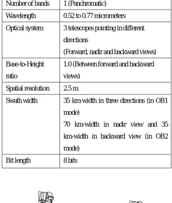
Table 2 PRISM principal specifications
Number of bands 1 (Panchromatic) Wavelength 0.52 to 0.77 micrometers Optical system 3 telescopes pointing in different
directions
(Forward, nadir and backward views) Base-to-Height
ratio
1.0 (Between forward and backward views)
Spatial resolution 2.5 m
Swath width 35 km-width in three directions (in OB1 mode)
70 km-width in nadir view and 35 km-width in backward view (in OB2 mode)
Bit length 8 bits
Fig.2 Observation modes
(Left:OB1 mode; Right:OB2 mode)
3.1 Verification of legibility
To map and revise 1:25,000-scale topographic maps using ALOS/PRISM images, it is necessary to collect, map and edit information on the latest geographic changes using various images—in the same way as with aerial photographs. In addition, ground verification must be conducted as needed (Fig. 3).
Therefore, we verified how much information on
©JAXA
©JAXA ©JAXA
changes in geospatial features, which are required for mapping and revising 1:25,000-scale topographic maps, could be collected and correctly interpreted from ALOS/PRISM images.
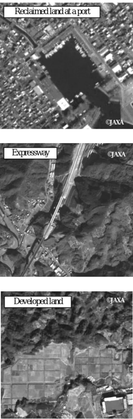
The result of the verification revealed that large-scale geospatial features such as expressways, reclaimed land at ports and developed land could be identified without difficulty (Fig. 4). With PRISM's resolution of 2.5 m, point features or small structures such as a lighthouse at a port, a tower on developed land, and a road divider cannot often be interpreted. In addition, legibility tends to decline in a region where features are located with high density on the ground (Fig. 5). Furthermore, it is also difficult to interpret a flat land surface without structures such as vacant land, rice paddies, fields and wasteland due to the lack of clearly identifiable textures and patterns (Fig. 6).
Fig. 3 Flow of preparation and revision of 1:25,000-scale
topographic map
The impact on legibility depends heavily on the resolution of the images. Other factors affecting legibility include image quality such as block noise and insufficient radiometric resolution.
Block noise results from JPEG compression, an irreversible compression applied to the observed images when the image data are transferred to the ground. This noise creates a regular 8×8 pixel block pattern on the images and adversely affects legibility (Fig. 7).
Fig. 8 shows an ALOS/PRISM image without radiometric correction (sensor's sensitivity: Gain 2) and its histogram. The entire image is dim and of low-contrast because the quantization bit rate is 8 bits, and the actual radiometric coverage is almost half the entire radiometric range and compressed toward lower range.
Fig. 4 Interpretation of large structures
Reclaimed land at a port
©JAXA
Developed land ©JAXA
Expressway ©JAXA
©JAXA
ALOS/PRISM image
Mapping edition
Unclear map symbols are determined.
Positions are locally measured.
Positions are measured using a plotting machine.
Map symbols are drawn. Information on geospatial features is acquired.
Map symbols are selected from interpretation.
Ground verification
Fig. 5 Interpretation of a dense residential area
Fig. 6 Interpretation of ground surface
Fig. 7 Block noise
Fig. 8 Image without radiometric correction, inset shows
the histogram (Sensor's sensitivity: Gain 2)
The image's resolution is fixed due to the specifications of the sensor, but the image quality could be improved. JAXA has continued to develop and utilize software for the reduction of block nose that employs a method developed by GSI, and to control the sensor's sensitivity based on seasonal changes in light intensity in order to improve the legibility of PRISM images. This has improved the image quality to some extent.
3.2 Verification of positional accuracies
GSI verified the positional accuracies for both orientation and plotting of ALOS/PRISM images (GSI, 2007). This report describes the outline of the GSI verification in Sections 3.2.2 and 3.2.3. This verification evaluates whether it is possible to apply ALOS/PRISM images (Processing level 1B1: Non-geometric corrected image) and RPC (Rational Polynomial Coefficients) data associated with the images to map and revise 1:25,000-scale topographic maps by orienting and plotting these images and data using a digital photogrammetry workstation.
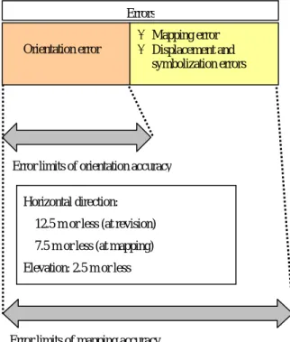
The relationship between the orientation and plotting accuracies can basically be considered as shown in Fig. 9. The orientation error results mainly from an RPC data-inherent error, GCP's (Ground Control Point: High-precision control point obtained from on-site surveys) coordinates error, a measurement error of GCP and tie points (points designating common location among images) on the images and so on. A combination of these factors must satisfy the limits of orientation accuracies specified in the operational regulations for a public survey (draft) (within 12.5 m [at revision] or 7.5 m [at mapping] in the horizontal direction, and within 2.5 m in the vertical direction). Conversely, a plotting error mainly results from an error of stereo measurement. A combination of orientation and plotting errors must meet limits of plotting accuracies (within 17.5 m (RMSE) in the horizontal direction, within 5 m (RMSE) for contour lines, and 3.3 m (RMSE) for spot heights).
The accuracies of 1:25,000-scale topographic maps are also affected, though only partially, by errors introduced by displacement and symbolization of geospatial features. In this report, mapping accuracies specified in the operational regulations for a public survey (draft) are employed as the
©JAXA
©JAXA
©JAXA
©JAXA
Noise is seen for each 8×8 pixel block = Block noise
error limit values for 1:25,000-scale topographic mapping. For reference, as the error limit values in the regulations (draft) were developed on the assumption of aerial photogrammetry, the direct application of these values to ALOS/PRISM images and other satellite images may not be always appropriate. This issue should be studied in the future.
Fig. 9 Relationship between orientation and mapping accuracies of
1:25,000-scale topographic map
3.2.1 RPC model
ALOS/PRISM individual images (processing level of 1B1) have parameter files called RPC data. If these parameters are used for an RPC model expressed as a rational polynomial given in Equation (1), the relation between image and geographic coordinates can be determined with relatively high precision. If coordinates (R1,
C1, R2 and C2) of the same location are measured on at least
two different images, the geographic coordinates (B, L and H) of the location can be calculated.
(
)
(
B
L
H
)
D
H
L
B
N
R
R R,
,
,
,
=
(
)
(
B
L
H
)
D
H
L
B
N
,
,
,
,
C
C C=
(
)
(
)
(
)
(
)
3 20 2 19 2 1 C 3 20 2 19 2 1 C 3 20 2 19 2 1 R 3 20 2 19 2 18 2 17 3 16 2 15 2 14 2 13 3 12 11 2 10 2 9 2 8 7 6 5 4 3 2 1 R , , , , , , , , H d H B d L d d H L B D H c H B c L c c H L B N H b H B b L b b H L B D H a H B a H L a BH a B a B L a LH a LB a L a BLH a H a B a L a BH a LH a LB a H a B a L a a H L B N + + + + = + + + + = + + + + = + + + + + + + + + + + + + + + + + + + = ・・・ ・・・ ・・・R, C : Image coordinates (row, column)
B, L, H : Geographic coordinates (latitude, longitude, ellipsoidal height)
(
1, ,20)
, , ,b c d i= K ai i i i : Approximate coefficients of RPC model*Latitude, longitude and ellipsoidal height are converted to projected coordinates and elevations as needed.
Fig. 10 RPC model
When geographic coordinates are calculated using Equation (1) in the previous section, these coordinates contain errors to some degree (a few meters to a few tens of meters in RMSE). An approximate expression with higher accuracy can be obtained by giving additional parameters to the above equation and determining the coordinates using GCPs. Shift parameters in the row and column directions on each image are added to Equation (2) as an additional factor.
(R2,C2)
(R1,C1) (B,L,H)
Image coordinates Geographic coordinates
(Latitude, longitude and ellipsoidal height)
(1)
• Mapping error • Displacement and
symbolization errors
Error limits of orientation accuracy
Error limits of mapping accuracy
≒Accuracy of 1:25,000-scale topographic maps (RMSE) Horizontal direction:
12.5 m or less (at revision) 7.5 m or less (at mapping) Elevation: 2.5 m or less
Errors
Horizontal direction: 17.5 m or less Contour lines: 5 m or less Spot heights: 3.3 m or less
(row, column)
©JAXA ©JAXA
©JAXA
(
)
(
B
L
H
)
D
H
L
B
N
s
R
R R R,
,
,
,
=
+
(
)
(
B
L
H
)
D
H
L
B
N
s
C
C,
,
,
,
C C=
+
C Rs
s ,
:Shift parameters (row and column directions) When this expression is used, at least one GCP is required to determine the shift parameters.The following section describes the verification of orientation accuracies using this approximate expression.
3.2.2 Verification of orientation accuracies
In order to verify ALOS/PRISM's orientation accuracies, GCP-based orientation tests were conducted in three regions, Tsukuba, Okazaki and Sakurajima. For each of these verification test sites, the number of GCPs to be used for orientation was varied. Assuming that the coordinates at verification points (points obtained from on-site surveys to verify orientation accuracies and not used for orientation) are true values, residuals of coordinates measured on an oriented image were calculated (Table 3).
Table 3 Orientation accuracies
Unit:m(RMSE) Number of GCPs None 1 3 6 Horizontal direction 18.25 2.34 2.08 2.11 Tsukuba Vertical direction 11.06 2.51 2.34 2.18 Horizontal direction 3.89 3.85 2.85 2.87 Okazaki Vertical direction 4.67 2.51 2.23 2.13 Horizontal direction 5.69 2.72 2.82 3.06 Sakurajima Vertical direction 9.07 3.26 2.38 2.43
Due to greater errors and their variations among different test sites for the orientation without GCPs, it can be seen that GCPs are required for orientation when 1:25,000-scale topographic maps are to be mapped and revised using ALOS/PRISM images. Three GCPs or more significantly reduce error variations within a range of about 2-3 m and 2-2.5 m in the horizontal and vertical directions,
respectively.
Based on these results of verification as well as the previous findings with photogrammetry, in order to satisfy the operational regulations for a public survey (draft), the orientation must be made as follows (Fig. 11).
-On the assumption of 100% overlap between the images, and the three-point method for aerial photographs, nine tie points are to be selected uniformly on each entire image scene.
-Obtain about six GCPs in consideration of redundancy to ensure the orientation accuracies specified by the regulations
Fig. 11 Configuration of tie points and GCPs
3.2.3 Verification of plotting accuracies
Under the following three types of verification, plotting accuracies of ALOS/PRISM images oriented using RPC data were measured.
1) Horizontal accuracy of plotting
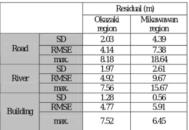
Roads, rivers and buildings in two regions, Okazaki and Mikawawan, were stereoscopically plotted. Next, the horizontal accuracy was calculated on the assumption that plotted data using 1:20,000-scale aerial photographs are true to verify the accuracy of the plotted data using ALOS/PRISM images (Table 4). For the comparison of plotted data, the coordinates of road centers, road ends, river centers, shorelines, building corners and so on were measured.
In Table 4, it can be seen that plotting errors (RMSE) in roads, rivers and buildings satisfy the plotting accuracy limit (within 17.5 m in the horizontal direction in RMSE). (2)
Table 4 Plotting accuracy (horizontal direction)
SD: Standard Deviation
2) Vertical accuracy by plotting
Errors in the vertical direction were calculated by comparing the spot height values that were measured by stereo plotting of the ALOS/PRISM images with the elevation values measured on 1:20,000-scale digital aerial photographs (Table 5). This verification was conducted in the Mikawawan region. In addition, for the measurement of spot heights, centers of white cross lines drawn in road intersections, where elevations are easily measured, were used.
From Table 5, it is seen that errors of spot heights (RMSE) reach 4.62 m in forward-nadir views and 3.12 m in forward-backward views, and the plotting errors substantially exceed the limit of elevations in the forward-nadir views (within 3.3 m at RMSE). Consequently, it was decided that it was not suitable to acquire spot heights by stereo plotting of ALOS/PRISM images.
Contour lines can be plotted because their errors meet the accuracy limit (within 5 m at RMSE), but it is necessary to plot the lines carefully due to their fairly large errors. The closest attention must be paid when contour lines are drawn with stereo pair images of forward (or backward)-nadir views that have a smaller B/H ratio (B/H ratio=0.5) than forward-backward views (B/H ratio=1.0) because it was confirmed that the errors became larger with smaller B/H ratio.
Table 5 Mapping accuracy (vertical direction)
Residual (m) Forward - Nadir Forward - Backward SD 2.45 1.83 RMSE 4.62 3.12 Spot height values max. 8.56 5.99
3) Quality of topographic features represented by contour lines
Fig. 12 shows a combination of two sets of contour lines from the Mikawawan region drawn by stereo-plotting of ALOS/PRISM images and aerial photographs. By making a comparison between these contour lines, the quality of the topographic features represented by the contour lines plotted with ALOS/PRISM images was qualitatively verified. The contour lines plotted with ALOS/PRISM images could not depict minute topographic features—unlike those plotted with aerial photographs. However, the ALOS/PRISM contour lines by and large depict topographic features required for the mapping of 1:25,000-scale topographic maps.
Fig. 12 Comparison of plotted contour lines (Only
index contour lines in the Mikawawan region) ※ Blue and green lines represent contour lines
plotted from 1:20,000-scale aerial photographs and ALOS/PRISM images, respectively.
4. Demonstration for revision of 1:25,000-scale topographic maps
The verification in Section 3 revealed that
Residual (m) Okazaki region Mikawawan region SD 2.03 4.39 RMSE 4.14 7.38 Road max. 8.18 18.64 SD 1.97 2.61 RMSE 4.92 9.67 River max. 7.56 15.67 SD 1.28 0.56 RMSE 4.77 5.91 Building max. 7.52 6.45
1:25,000-scale topographic maps could be mapped and revised using ALOS/PRISM images, but with partially conditional legibility and positional accuracies.
However, it is necessary to review the adequacy of legibility and positional accuracies meeting the requirements of the operational regulations for a public survey (draft), and also the efficiency and performance of actual works, in order to actually use them on a full scale. Therefore, the following demonstration activities were implemented.
4.1 Consideration on orientation method suitable for actual operations
The result of the verification in Section 3.2.2 is that the number of tie points required was nine, and that the number of GCPs required was six.
It does not take a lot of time and labor to measure nine tie points with a digital photogrammetry workstation. But the orientation of one image scene with spare points requires that more than six GCPs should be measured on the ground. In light of the extent of one full scene (35 x 35 km) and the distance required to travel in the area, this requires significant time and labor. For this reason, an orientation method that minimizes ground measurements and provides a practical workload was developed.
From Table 3, it is seen that the orientation with one GCP in the horizontal direction sufficiently meets the limits of the regulations (draft). Because the limit for the vertical direction is more rigorous than that for a horizontal direction, however, methods must be devised to constantly ensure sufficient vertical accuracy.
Hence, assuming that only one GCP is available from the ground measurement, we examined a method for using elevation information on a 1:25,000-scale topographic map to ensure vertical accuracy. It is easy to find appropriate elevation values on 1:25,000-scale maps for an area as large as an ALOS/PRISM scene, which reduces the workload of GCP acquisition on the ground.
Fig. 13 represents a graphic plot of coordinate residuals that were measured on the image rectified with the use of one GCP and a number of spot heights (varying from one to 10 points) and with coordinates at verification points as true values. The result shows that sufficient vertical accuracy could be achieved with three or more spot heights
measured on the topographic maps. Also in consideration of the results in Section 3, the following orientation method could be employed to ensure the orientation accuracies specified in the regulations (draft) and enable operational mapping activities (Fig. 14).
- On the assumption of a thee-point method for aerial photographs, nine tie points must be obtained uniformly on the entire scene based on almost 100% overlapping. - The orientation must be made with at least one GCP, and at least five spot heights on 1:25,000 topographic maps. - One GCP can be placed on any position of the image, but the GCP and spots heights must be uniformly configured through the image scene.
0 0.5 1 1.5 2 2.5 3 3.5 4 1 2 3 4 5 6 7 8 9 10
Number of spot heights
Re sidu al( m ,R M S E )
Horizontal direction (Akiyoshidai) Vertical direction (Akiyoshidai) Horizontal direction (Hamanako) Vertical direction (Hamanako)
Fig. 13 Residuals of orientation with a number of spot heights
:Tie point : GCP : Spot height
Fig. 14 Configuration of tie points and spot heights for
4.2 Consideration as to work efficiency and performance In the verification of legibility in Section 3.1, it was concluded that small structures and other minute geospatial features could not be interpreted in ALOS/PRISM images due to the limitation of spatial resolution of 2.5 m and the effects of systematic noise on image quality, but it was found that changes of large geospatial features can be identified with decent interpretation.
Here, in order to review the efficiency and performance of the work required for the revision of a 1:25,000-scale topographic map, ALOS/PRISM images in the area of Yamato, Sendai, were rectified, and initial change detection (extraction of changes in geospatial features and interpretation of the images), ground verification and plotting were conducted using the same process as in actual map revision procedures. For comparison, the same procedures were taken for 1:20,000-scale color aerial photographs.
If aerial photographs, as one of the main traditional means of map revision, and ALOS/PRISM images are separately used for the work, and the aerial photographs-based result is compared with the ALOS/PRISM-based result, the efficiency and performance of work using ALOS/PRISM images can be evaluated.
The result of initial change detection, as described in the results on the verification of legibility, indicated that while some types of features, depending on their size or conditions, were difficult to interpret in the images, large geospatial features could be identified almost without problems (Fig. 15), and the initial change detection procedure was successfully completed. Due to the fact that the images have more hard-to-interpret features than the aerial photographs, the time required to organize and summarize the results of the change detection shown in Fig. 15 is slightly increased. However, this factor is not considered to greatly affect the efficiency and performance.
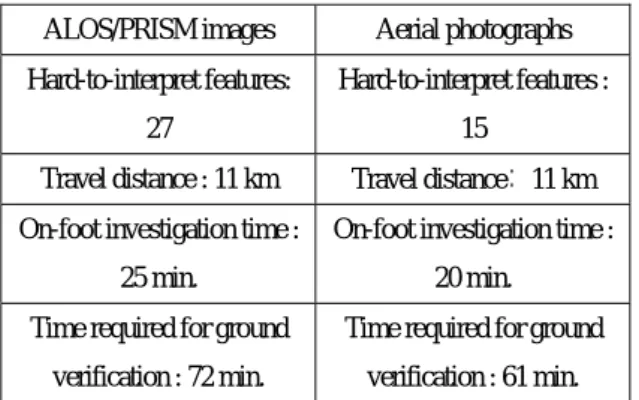
Next, in order to review the efficiency of ground verification, hard-to-interpret features were checked in the field to compare the number of the locations with travel distances and times during the ground verification (Table 6). The ALOS/PRISM images had many locations that needed to be checked in the field, but the total travel distances to these locations were almost the same for both cases. For this
reason, the time required for ground verification of the ALOS/PRISM images was not greatly different from that of the aerial photographs, resulting in the same work efficiency and the same output as aerial photographs. However, those areas with many hard-to-interpret features due to crowded features in residential areas required a lot of time for ground verification, and were found to be inappropriate for the work using ALOS/PRISM images.
Fig. 15 Results of initial change detection and ground verification with ALOS/PRISM images
(Red:Initial change detection; Blue: Ground verification)
Table 6 Comparison of efficiencies of ground verification
ALOS/PRISM images Aerial photographs Hard-to-interpret features:
27
Hard-to-interpret features : 15
Travel distance : 11 km Travel distance: 11 km On-foot investigation time :
25 min.
On-foot investigation time : 20 min.
Time required for ground verification : 72 min.
Time required for ground verification : 61 min.
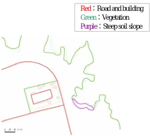
When the plotting result from ALOS/PRISM images were compared with that from aerial photographs (Fig. 16), it was found that the ALOS/PRISM images could not provide the exact shapes of changes such as the minute geometries of buildings, and the absence or presence of small steep soil slopes as much as the aerial photographs, but it was also demonstrated that features with a size required for revision of a 1:25,000-scale topographic map could be
identified and plotted without much difficulty. However, features that cannot be clearly identified require some time for evaluation, and potentially additional ground verification, which would reduce work efficiency. Before plotting, it is necessary to ensure thorough ground verification and collection of references, and establish map symbols to be drawn.
Fig. 16 Comparison of plotted results
(Deep color : ALOS/PRISM image; Light color: Aerial photo)
If ground verification of areas with non-dense structures is correctly made with a focus on large-scale features with ALOS/PRISM images in a series of revision process of initial change detection, ground verification and plotting, the 1:25,000-scale topographic maps can be revised with almost the same efficiency and performance as with aerial photographs.
5. Applications of ALOS/PRISM images
GSI introduced a digital photogrammetry workstation that employs the RPC model in March 2008 to support the more efficient development and revision of 1:25,000-scale topographic maps, and started full-scale use of ALOS/PRISM images.
We reviewed advantages of ALOS/PRISM images that can serve as a means for more effective and efficient revisions of 1:25,000-scale topographic maps, in comparison with various other methods such as aerial photographs, reference maps and on-site surveys (Table 7).
Table 7 Applications of ALOS/PRISM images
ALOS/ PRISM's images Preparation and revision methods Applications Si ngl e i m ag e mappin g S tereo mapp ing Aerial pho tograp hs Refer enc es , s ite s u rveys , et c.
Available new aerial photos × × 〇 × Processing of contour lines
(Large developed land, cut-and-fill road, etc.)
× 〇 ― △ Many large changes △ 〇 ― △ Non-processing of contour lines (Port reclamation,
river repair, etc.) Few small changes 〇 △ ― △ Unavailab le new aerial photograph s
Locations where aerial photographs are hard to take and on-site surveys are hard to
conduct
△ 〇 ― ×
○ : Acceptable
△ : Approved (Partially approved) × : Unacceptable, not approved
※ It should be noted that the criteria are not absolute.
When there are new aerial photographs available, they should be used as they have a higher resolution and greater versatility than ALOS/PRISM images and are easily processed. On the other hand, when contour line processing is needed, the contour lines are not often represented in reference maps and may not be easily obtained even through on-site surveys. In addition, sometimes a great deal of large changes cannot be supported by reference maps and on-site surveys. When changes of ground features are relatively small, no reference maps exist in most cases. In these cases, the map can be revised in an effective manner by using ALOS/PRISM images. In cases where it is difficult to take aerial photographs from an airplane, and where an inaccessible and isolated land is being investigated, ALOS/PRISM images and other satellite images are effective in revising maps.
Red:Road and building
Green:Vegetation
6. Examples of application for revision of 1:25,000-scale topographic map
6.1 Example of collection of changes of geographic information
As the information in 1:25,000-scale topographic maps becomes outdated over time, it is necessary to revise changed features. For the revision of a map, as shown in Fig. 17, these changed features are extracted, while the features are interpreted to find out what have changed. Because of the wide-area coverage of ALOS/PRISM images that are frequently acquired at regular intervals, it is possible to effectively collect the changes of features for the revision of the 1:25,000-scale topographic maps.
Fig. 17 Example of change detection with ALOS/PRISM imagery
6.2 Example of revision of 1:25,000-scale topographic map
If changed features are collected from ALOS/PRISM images, and map symbols for the changed features are determined from ground verification and reference maps, the map symbols are drawn at proper positions to complete the revision of a 1:25,000-scale topographic map. Some examples of map revision with ALOS/PRISM images are given below.
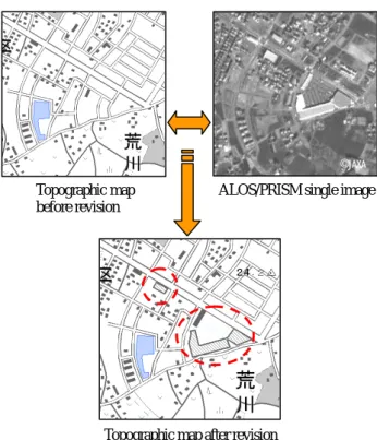
6.2.1 Example of map revision using a single ALOS/PRISM image
When the changed features are located on relatively flat ground, one ALOS/PRISM image is enough to revise a map based on the changed features by overlaying the map on top of the image with a map-compilation software application and tracing the changed features. Figs. 18 and 19
show a large building and a road that were detected as changes using a single ALOS/PRISM image and used to revise 1:25,000-scale topographic maps. ALOS/PRISM images have the advantage of making map revision easier and simpler than aerial photographs, which require a digital photogrammetry workstation for orientation and stereo plotting.
Fig. 18 Map revision of a large building using a single image
(1:25,000-scale topographic map “Tsuchiura”)
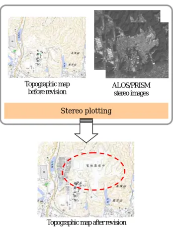
6.2.2 Example of revision using ALOS/PRISM stereo image pair
Fig. 20 shows an example where an ALOS/PRISM stereo image pair is oriented using a digital photogrammetry workstation that can employ the RPC model, and a 1:25,000-scale topographic map is revised by stereo plotting. Because stereo plotting enables the acquisition of contour lines, it is possible to revise developed land with changed geospatial features and a large cut-and-fill road. Furthermore, due to the improvement in legibility due to the stereoscopic view of the image pair, complicated revision of the map can be done with high precision, and the number of hard-to-interpret locations can be reduced, resulting in a reduction of the time required for ground verification and reference data collection.
Aerial photograph (Taken in 2001) ALOS/PRISM image (Observed in 2006) Stadium ©JAXA Topographic map before revision
ALOS/PRISM single image
Topographic map after revision
Fig. 19 Map revision of a road using a single image
(1:25,000-scale topographic map “Yatabe”)
Fig. 20 Map revision of developed land for housing by stereo
plotting(1:25,000-scale topographic map “Tannowa”)
6.2.3 Notable example I—Map revision for Io To Island 1:25,000-scale topographic maps are prepared based on consistent specifications for all parts of the country, even for remote islands that are located far away from the mainland. As it is difficult to take aerial photographs of these remote islands, ALOS/PRISM images, which can be provided for any place on the Earth regardless of the location, can be used effectively as a means for revising topographic maps.
A 1:25,000-scale topographic map for Io To Island, which was first issued in 1982, was revised for the first time in 25 years and reissued on September 1, 2007. This was the first case in which ALOS/PRISM images were used for the revision and issuance of a 1:25,000-scale topographic map.
In this example, after the images were imported into map-compilation software, changed features including an airport, roads, buildings (Fig. 23) and coastline (Fig. 24) were revised using the results of ground verification and on-site surveys. Other high-resolution satellite images were also used as needed.
Fig. 21 ALOS/PRISM image used for revision of Io
To Island
Fig. 22 ALOS/PRISM image used for revision of Io
To Island (partial enlargement) Topographic map
before revision
ALOS/PRISM single image
Topographic map after revision
©JAXA
Topographic map after revision Topographic map before revision Stereo plotting ALOS/PRISM stereo images ©JAXA
Part of outdated topographic map (issued on March 30, 1982)
Part of revised topographic map (issued on September 1, 2007)
Fig. 23 Map revision for Io To Island (1)
(1:25,000-scale topographic map “Io To”)
Fig. 24 Map revision for Io To Island (2)
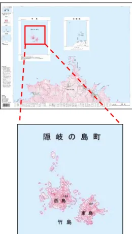
6.2.4 Notable example II—Mapping of Takeshima In places such as Takeshima, where it is difficult to take aerial photographs and access in person to carry out ground verification and on-site surveys, ALOS/PRISM images and other satellite images are the only option available for the development of 1:25,000-scale topographic maps. Therefore, ALOS/PRISM and other satellite images were employed when a topographic map of Takashima was prepared for the first time as an inset map for the 1:25,000-scale topographic map of “Nishimura,” issued on
December 1, 2007 (Fig. 25).
Fig. 25 Preparation of 1:25,000-scale topographic
map of Takeshima
(1:25,000 topographic map “Nishimura”)
Before ALOS/PRISM images became available, high-resolution satellite images from other sources could have been used to draw the geometries and topographic features of islands and interpret them in detail. But due to the difficulty in accessing Takashima, GCPs were not available, and locations on satellite images could not be determined with high precision.
Geographic coordinates of Takeshima can be determined with RPC data when ALOS/PRISM images are employed, but the positional accuracies could contain large errors due to the unavailability of GCPs. Therefore, the following special method was developed to determine the geographic coordinates of the island with higher accuracy.
ALOS/PRISM is an optical sensor with three systems comprising forward, nadir and backward views. A positional relationship between the sensor's three axes and the body of ALOS is decided by calibration/verification (Fig.
The coastlines surrounded by red dashed lines were revised
26). In addition, as GCPs can be obtained within images for Yamaguchi and Kagoshima, the attitude and position of ALOS can be calculated with high accuracy when the satellite observes the images of Yamaguchi and Kgoshima. Furthermore, the forward view for Yamaguchi and the nadir view for Takeshima are simultaneously observed, while the forward view for Kagoshima, the nadir view for Yamaguchi and the backward view for Takeshima are observed at the same time. Consequently, the attitude and position of the satellite when the satellite observes Takeshima are the same as those when it observes Yamaguchi and Kgoshima. As mentioned above, as the positional relationship between ALOS/PRISM's three-direction sensor and the body of ALOS is fixed, the sensor's viewing direction toward Takeshima is determined once the other viewing directions are fixed. Based on the above consideration, geographic coordinates of Takeshima can be determined with high precision by stereo measurements using the images of Takeshima observed from two directions. The same method was applied to a pair images observed in different periods, and the difference between the geographic coordinates measured from these two image pairs for Takeshima was a few meters. Additionally, the same method was applied to measure geographic coordinates of other known areas, the result proved the viability of the method. Therefore, this method was adopted to determined the location of Takeshima (Figs.26, 27).
Fig. 26 Configuration of ALOS/PRISM
Fig. 27 Method for measurement of geographic coordinates of Takeshima
7. Conclusion
GSI and JAXA have completed a series of joint studies to verify and demonstrate the applications of ALOS/PRISM images for mapping applications. Based on the results of these studies, GSI has started full-scale use of ALOS/PRISM images for revising 1:25,000-scale topographic maps as shown in the above examples. Recently, it has become more common to continuously revise maps for changes of major features and immediately release them via the Internet. Consequently, GSI plans to make further use of ALOS/PRISM images for the extraction of changed features and for the revision of 1:25,000-scale topographic maps, maximizing the benefits of the images that can be acquired for anywhere and with high frequency.
Acknowledgments
This study was conducted as joint research by the Geographical Survey Institute and the Japan Aerospace Exploration Agency (JAXA). ALOS/PRISM images used in this study were provided by JAXA. We extend our thanks JAXA for their cooperation.
©JAXA
Take- Yama- Kago- shima guchi shima
Take- Yama- Kago- shima guchi shima
ALOS ALOS Satellite's heading direction
Backward v N adir Forwa rd Stereo measurement
Calculate the satellite's inclination and position more accurately with GCPs
GCP available GCP available
N
adir Forwa
References
GSI(2007): Report on verification of the accuracy of ALOS/PRISM's RPC model by digital photogrammetry workstation, Geographical Survey Institute's technical information C1-No.372.
Ishizeki, T. (2008): Map revision by "Daichi" – Utilization of ALOS/PRISM –, 37th Geographical Survey Institute Report Meeting, Geographical Survey Institute's technical information A・1-No.332, 63-71.
Jaxa (2005): ALOS User Handbook, Japan Aerospace Exploration Agency.
Jaxa (2006): ALOS Data Guidebook, Japan Aerospace Exploration Agency.
Uchiyama, Y. (2007): Application of ALOS/PRISM Images to Revision of 1:25,000 Topographic Maps, Geodetic Dept.'s technical report No. 17, Geographical Survey Institute's technical information C2-No.18, 15-24.
Verification of Topographic Road Centerline Data Using ALOS/PRISM Images:
Implementation
Hidenori FUJIMURA, Hidekazu MINAMI, Takenori SATO and Takahiro SHIMONO
Abstract
Elimination of displacement due to map editing inherent in road centerline data of the New Topographic map Information System (NTIS) is implemented. Panchromatic satellite images from ALOS/PRISM are used in the process. Histogram analysis of gray value profiles parallel to the roads is employed. The true-position candidate is selected by supervised classification of histograms using support vector machine (SVM) method. According to the experiments with the Japanese NTIS road centerline database, the proposed method reverses the displacement of approximately 50% of the road features, while a further 20% of the road features are validated as already located at the true position. The proposed method is proved to be useful for German Amtliches Topographisch-Kartographisches Informationssystem (ATKIS) road database. This indicates wider applicability of this method to various geographic regions.
1. Introduction
In many countries digital landscape models (DLM) of the national mapping agencies provide a fundamental positional reference for a multitude of tasks related to geospatial information. The quality of this positional information is thus of prime importance. The DLM have usually been set up based on the requirements of a topographic map of similar content. Recently, independent sources of positional information, such as the global positioning system (GPS), which inherently has a very high geometric accuracy, have gained in popularity and are being used today for many applications such as car navigation. In order to provide the user of a DLM with the possibility to overlay his GPS data with the DLM and derive meaningful conclusions, both need to be at the same level of geometric accuracy. To fulfill this requirement, it is essential in many cases to enhance the geometric accuracy of the existing DLM.
The Geographical Survey Institute (GSI), the national mapping agency of Japan, had digitized its topographic map data at a scale of 1:25,000 to generate a printing quality image database (Sato et al. 1995). Original drawings of the topographic maps were scanned and stored in raster form. After this raster-based system had been realized, all the data were vectorized and stored in vector form into a topographic map information system named NTIS (Ohno et al. 2002). As a result, both the raster data and the NTIS data still contain effects from map editing which
stem from the topographic map.
According to the specifications of the Japanese topographic map 1:25,000 in paper form, the geometric accuracy of NTIS features is defined to be 12.5m in general. The geometric accuracy is allowed to be degraded down to 25m in case of cartographic map editing. For the reasons explained above, the geometric accuracy of the NTIS data needs to be improved.
For the task of removing the effects of map editing, information of additional data sources is necessary. For urban areas, conflation with existing larger scale vector data is possible and will achieve a high level of automation. Currently, the GSI investigates methods to merge these heterogeneous vector datasets.
This paper focuses on the automatic reversal of generalization in rural areas. For these regions topographic data with larger scale are rarely available. Hence, satellite imagery is used for comparison with the database information. For this project up-to-date imagery of the Advanced Land Observing Satellite (ALOS) acquired with the Panchromatic Remote-sensing Instrument for Stereo Mapping (PRISM) was used.
Due to the importance of the road network for the users, and because the road network forms a geometric frame for all other features, this research aims at a reversal of feature displacement inherent in NTIS road features. For this task, an analysis based on histograms of profiles parallel to the road in the image data is suggested. The geometric
position and shape of each NTIS road feature is considered as prior information.
The aim of the work is to develop a new method which can be used at GSI to process the whole NTIS database of Japan as automatically as possible in a time frame of approximately 12 months. This paper reports on results achieved for the described task. Japanese as well as German datasets were processed in order to demonstrate that the algorithm can be transferred across different regions in the world.
2. Related Work
In this section, a selection of existing approaches for updating and verification of existing road databases with a practical background is described. There are two aspects of major interest for us: Firstly, the way other authors incorporate existing prior information, secondly, the road model used and the subsequent handling of road features that do not conform to the model. The second aspect is important to make our method to be practical since our method needs to be robust against large-size input.
In early work Bordes et al. (1995) suggested to guide road extraction for the BDTopo of the French Institut Géographique National (IGN) by information from the less detailed BDCarto. The accuracy of the result is evaluated using a matching strategy between the two datasets. Wiedermann and Mayer (1996) check roads which are available in a database by investigating the gray value profiles perpendicular to the road axes.
Klang (1998) proposed a semi-automatic system for an enhancement of the Swedish road database based on a comparison with satellite imagery of SPOT and Landsat. The approach detects the position of road junctions by different template matching method in the image within a tolerance radius around the given position. Based on this result the nodes are used as seed points for an active contour model applied to every road feature of the database. Finally, a comparison of the extraction result and the corresponding database object provides the human operator with a number of potential objects for the updating process. Thus, the extracted roads are not automatically included in the database. The system was extended in relation to the task of the National Topographic Database of Geomatics Canada
(Fortier et al. 2001). The enhanced quality of the extracted junctions was used to include the detected roads directly in the database and make the whole system fully automatic.
Another relevant project in our context is the Automated reconstruction of Topographic Objects from aerial images using vectorized Map Information (ATOMI) of Switzerland (Zhang 2004). The approach makes extensive use of prior knowledge derived from the existing database, i.e. geometries and attributes as well as topological information of the given road network. Additionally, context information about local background objects is used to define an adaptive road model for urban and rural areas. The automatic analysis is realized using stereo color aerial images combined with DSM information. The road model is based on gray value gradients but uses also aspects of area classification to consider shadow and occulusion by context objects.
The WiPKA-QS project deals with the automatic quality control of the German authoritative topographic reference dataset ATKIS-DLM and the MGCP (Multinational Geospatial Coproduction Program) dataset using aerial or satellite imagery (Gerke et al. 2004). Following the same main strategy proposed by Klang (1998), selected road features with high evidence for correctness are processed automatically. Similar to the approach proposed by Zhang (2004), the road model is mainly gradient based and is adapted using prior knowledge from the database. WiPKA-QS enables a speed-up of about a factor of 3 as compared to manual quality control (Busch et al. 2004). More recent work in this project deals with analyzing histograms of road profiles to improve the performance (Ziems et al. 2007).
Active contour models, used by Grün and Li (1997) to cite a case, seem also to be applicable for this task. Snakes are deformable objects and thus can adapt naturally to road features in image space. In general, however, snakes suffer from the need for a good initialization and thus require a relatively high number of seed points. Butenuth (2007, 2008) showed that the network topology can be used instead of accurate seed points and can overcome many limitations of traditional snakes. A precision improvement of the Japanese 1:25,000 vector data using snakes was already investigated (Uetaki et al. 2006). The algorithm achieves
good performance in suburban and rural areas, but it is rather slow and needs high-resolution aerial imagery which is costly.
3. Data Sources
3.1 Japanese NTIS and ALOS/PRISM
As mentioned above, the road data of the NTIS have a positional accuracy of 12.5m. In case of cartographic generalization, the positional accuracy can degrade down to 25m. An important property of the NTIS road features is that most of them are straight. Fig. 1 shows the number of composing points for each road feature in our test site. According to this figure, nearly 50% of the road features are represented with only two points. From experience we know that this is a consequence of the fact that the actual roads in the real world in a typical Japanese open landscape are mostly straight, and not a result of simplification as apart of the cartographic map editing.
Fig. 1 Number of composing points for each road feature
in our test site (50.8km2 in open landscape).
Fig. 2 shows an ALOS/PRISM image superimposed with NTIS road features. ALOS/PRISM is a 2.5m resolution panchromatic sensor with a ground coverage of 35×35km2. An ortho-rectified image is used in our study. The horizontal positional accuracy of the georeferenced images is around 2.5m (Mizuta et al. 2007). Clear differences in geometry due to feature displacement can be observed in Fig. 2.
Fig. 2 Typical difference of ALOS/PRISM imagery and NTIS road
features (light blue).
3.2 German ATKIS and IKONOS
A second set of data sources was considered in our work, to check if our method can be employed in different landscape, and to evaluate our method with additional data sources. This set consists of IKONOS ortho-rectified images and road database, which is derived from the Digital Landscape Model (DLM) of the German Authoritative Topographic Cartographic Information System (ATKIS). The main difference to the first set (NTIS and ALOS/PRISM) is that ATKIS DLM road features have a geometric accuracy of 3m and have not been subject to cartographic map editing. Consequently, there is no direct demand for detecting a shift of ATKIS DLM road features. However, the quality of the proposed algorithm can be measured, because we can utilize the validated database information for external evaluation. This second dataset is also aimed at investigating the applicability of the proposed method to images of a higher resolution.
The available IKONOS scenes consist of the panchromatic and four spectral bands. For our investigation, pan-sharpened images with a ground resolution of 1m were used. The imagery contains three different German regions called Hildesheim, Weiterstadt and Ulm. The images are obtained in different season and the regions belong to different terrain types.
4. Methods 4.1 Model Selection
In order to solve the stated problem, we had two major points to decide; (a) a model for cartographic generalization of the road features, and (b) a model for roads
to be extracted from images must be selected. Both models can also be combined, e.g. in a snakes-based approach. Although snakes have a number of attractive properties (see above), they were judged to be too complicated, and to be too slow for our aim. Also, the fact that snakes can deform during the processing was not an advantage in open landscapes in Japan, where most of road features are just straight.
According to the fact that most road features of interest are straight, we employed an assumption that road features are shifted perpendicular to the road direction. This model is local and very simple, which makes it attractive from a practical point of view. However, according to this model, the topology of the road network will be destroyed. Since road topology is one of the major points to be preserved, a post-processing step was designed: the one-dimensional shifts of all edges incident to a node are considered to derive the final two-dimensional node shift. The shifted nodes are then topologically connected in the same way as before. There may be extreme cases where edges cross each other due to erroneously large shifts. But, in our experience, in most cases the topology does not change, when applying the described method.
The second issue is the extraction of road features from the image. As was discussed in section 2, a number of approaches have been suggested for this task, many approaches use prior database knowledge (the position, the direction, the length, the width of the road feature, etc.) and consider the road as a line. While we also use the information from the database, we suggest an alternative method and model for road feature extraction. We look at different gray value profiles parallel to the database road feature in a buffer of a certain width. The width is related to the geometric accuracy of the database and the amount of potential effect from map editing. Given an appropriate distance between the profiles, one of them describes the road feature, and the other profiles lie to the left or lie to the right of the road feature. The profiles outside the road contain gray values of the road neighborhood. Eventually, out task is to select the profile belonging to the road feature; the problem can be solved by classifying all profiles into the two classes called road or non-road.
In this way we turn the feature extraction problem
into a classification problem. After defining an appropriate feature space, we can use standard classification algorithms for remote sensing or pattern recognition. We selected the support vector machine (SVM) classifier, as it has proven to be a very successful algorithm (e.g. Vapnik 1998, see also Mallet et al. 2008). The open-source SVM library LIBSVM (Chang and Lin 2001) was used. Instead of outputting the label of the class, the SVM is set to output the estimated confidence to belong to the class (see Wu et al. 2004 for details).
According to some investigation on the gray value profiles, we define a road as follows:
(a) The road has a profile histogram which is dissimilar to those of all its neighbors, while the neighboring histograms are similar to each other. While we need a certain degree of internal homogeneity of the left and the right neighborhood, the two sides of the neighborhoods need not to be similar.
(b) The road surface is homogeneous, therefore the histogram of the road profile has low entropy. Also, the average value of the road profile is different from that of the surroundings.
While this definition is not always valid in urban scenes, it is generally satisfied in open landscape, where we see priority in this task.
4.2 Pre-Processing
A major prerequisite of the suggested approach is that the database information is used to define the approximate position and shape of every road feature in the image. The NTIS has a number of short road features which can be merged as a part of a longer road feature. As the first step, these short features are linked to make the histogram from the gray value profile more robust and reliable. Our experience showed that we need road features with a length of at least 60 pixels.
In the dataset from NTIS, such short features make up 28% of the road features in number. Most of such short road features are connected. In the test area in Germany, 5% of the road features are subject to the preprocessing.
Fig. 3 Idea underlying the proposed algorithm: for one road feature (left), the different profiles and the resulting gray value histograms
are depicted. As can be seen, the green histogram representing the road is distinctly different from the neighboring histograms. As compared to the position of the database road shift at shift = 0, the road feature in the image is located 7.5m to the left.
4.3 Road Detection by Histogram Classification Overview
Fig. 3 shows the idea of histogram analysis of the proposed algorithm. The different profiles and the related histograms of a road feature are shown. In this case, the actual road is located at a shift of 7.5m to the left of the road feature in the database (the line depicted at a shift of 0). The overview of the main algorithm is described as the following:
1. Create candidates for road features in approximate positions by use of database information. Candidates are generated in a buffer parallel to the line connecting the start and the end point of the database road. The range of possible shifts is determined according to the accuracy specification of the database and potential displacements due to generalization. In this work, the range is set to -30m to 30m because the limit of the feature displacement is 25m (see above). We included a 5m margin on either side because we need some background area to separate roads from the background. The step size of the shift is determined considering the precision of data sources. In our work, the step size is 2.5m or one pixel. Therefore, we obtain 25 candidates for each given road feature.
2. Calculate the histogram of line pixels belonging to each candidate profile. Road width attributes are considered when available by defining the width of the region for which the histogram is calculated.
3. Calculate a feature vector for each candidate profile, as explained below, from the histograms.
4. Determine the shifts manually for a small number of road features. These shifts area used to train the classifier based on a support vector machine.
5. Classify all histograms using the classifier.
6. Choose the actual road features from the output of the classifier.
Feature Vector
The feature vector consists of a number of features chosen to differentiate the road from the surroundings. All features are calculated from the normalized histogram
) (g
Hs where s is the shift and g is the gray value. The
components of the feature vector are:
1. ‘Sum of similarity of histograms (SSH)’ between one histogram s and all other histograms t in the neighborhood. The histogram similarity is expressed using the Bhattacharyya distance BC(H1, H2) (Bhattacharyya 1943, Fukunaga 1990):
∑
− = − = S S t t s BC s SSH( ) ((1 δ ,) )∑
∈ = G g t s g H g H BC ( ( ), ( )) (1)where δ denotes the Dirac function. Fig. 4 explains the idea of SSH, an example is shown in Fig. 5: In a typical open landscape in Japan, the SSH steeply decreases from
around 20 to less than 10 when the histogram Hs(g) describes a road feature.
Fig. 4 Explanation of SSH: histograms with many similar
partners have a large SSH while unusual histograms (such as those of road features) have a small SSH.
Fig. 5 A plot of SSH, a road is situated at a shift of 2.5m.
2. Average brightness M(s) along the profile:
∑
∈ ⋅ = G g s g H g s M( ) ( ( )) (2)This feature is chosen due to the fact that the average gray values of the road and the surroundings are assumed to be different. The average was normalized by dividing it by 256, as the radiometric resolution of the image was 8 bit. 3. Entropy of the histogram:
∑
∈ ⋅ − = G g s s g H g H s E( ) ( ( ) log ( )) (3)This feature is chosen to include information about the texture. If the area is homogeneous as a road is assumed to be, the entropy will be low. The entropy was normalized by dividing it by 8 (the maximum entropy given the radiometric resolution of 8 bit).
4. Normalized rank, i.e. the index of the value in the sorted list of values for all 25 candidates, of the SSH. All rank values were normalized by dividing the actual rank by the
number of candidate profiles.
5. Normalized rank of average gray value. 6. Normalized rank of the entropy.
We added the normalized rank of the first three feature vector components. This is because rank features significantly help in separating the two classes according to our experience.
Consequently, six feature vector components are calculated for every available spectral band, i.e. in case of the PRISM imagery, the dimension of the feature vector was 6, while for the IKONOS imagery with four spectral bands the dimension of the feature vector was 24.
By normalizing all feature vector components to a range between 0 and 1, numerical problems in the following classification are minimized.
Shift Estimation
For every considered profile the output of the SVM is the value describing the confidence that the considered profile stems from a road feature; an example can be seen in Fig. 6. According to experience the maximum with a confidence value higher than a pre-defined threshold is chosen to estimate the shift. The confidence value is also used to assess the reliability of the estimated shift: if the detected maximum confidence value is too small or side maxima exist near the maximum, the shift estimation is labeled unsuccessful. Possible reasons are that the cartographic map editing of the feature was more complex than a simple shift or that the assumed road model does not comply with the specific feature. In these cases, a human operator must interactively carry out the appropriate de-generalization of the road feature.
Fig. 6 Confidence values as a function of shift. In this
4.4 Adaptation to Database Topology
Because road features are shifted individually, the (assumingly correct) topology of the road network from the database is in general destroyed. Since a correct topology is obviously of major interest, e.g. for routing applications, post-processing to recover the topology of the road network is required.
We consider each node individually and compute the node shift using a weighted least-squares approach with the shifts of all road features incident to that node as observations. The discrepancies between the different individual shifts are then minimized, taking into account that each shift only contains information about the shift direction orthogonal to the road feature. The weights we use correspond to the confidence values computed before. The resulting shift is then applied to the node. Subsequently, a Helmert transform is computed for each road feature between two nodes (for straight features, this is equivalent to connecting the two shifted nodes by a straight line). In this way the topology is preserved locally, and only in rare cases, e.g. if the sequence of roads changes due to extremely different shifts of two neighboring nodes, the topology changes globally. In the test examples, this case did not show up. Therefore, for the time being we accept this inconsistency for reasons of algorithmic simplicity.
5. Results and Discussion
For the evaluation of the proposed method, reference datasets were manually extracted from the images. These datasets were supposed to be correct. For the Japanese test area we generated the reference dataset ourselves. For the German test areas we used an independent dataset, obtained from the German Federal Agency for Cartography and Geodesy (BKG). This reference dataset was initially produced for evaluating the quality assessment system WiPKA-QS (Gerke et al. 2004).
5.1 Japanese NTIS Data
The necessary training data were collected in a small area of 4.5km2 in the image. The number of road features in the training set was 74. The trained model has a regression ratio of 99.4%.
Fig. 7 shows our results for the area depicted in Fig.
2. For road features in green, the shift was validated by the human operator. For the red ones no reliable result could be computed or the human operator found it to be incorrect. In comparison with Fig. 2 we ca see that most road features are moved to the correct position. Table 1 shows the statistics of the result for the test site. Only 21% of the road features were found to be at the correct position before the shift estimation. However, after applying the described algorithm, an additional 52% of the road features could be corrected. Only the remaining 27% of the road features have to be processed by a human operator.
Fig. 7 Result for NTIS data (green: correct, red: incorrect).
Table 1 Result for Japanese NTIS/PRISM in selected open
landscape (50.8km2, 569 road features).
correct without shift 21% correct after shift reversal 52%
incorrect 27% The reliability of the algorithm was checked in the
following way: if a human operator could find a road feature at the place of the shifted road, the result was termed “accepted”, otherwise it was termed “rejected”. The result of this evaluation is shown in Table 2. Nearly 98% of the detected road features comply with the decision of the human operator, thus the success rate of the developed method is very high.
A typical false-positive decision is shown in Fig. 8. A row of buildings is recognized as a road. We will try to detect this error in the future by using building data and by applying an additional evaluation step, in which shifts of topologically connected road features are considered simultaneously.
Table 2 Reliability of the results (here, only the correct
features of the first test were considered).
system human operator correct shift accepted 97.6% rejected 2.4%
Fig. 8 false positive result: a row of buildings recognized as a road.
5.2 German ATKIS Data
As mentioned above, the additional test with the German ATKIS data was carried out to demonstrate that the developed algorithm can be transferred from one geographic region of the world to another one. Since ATKIS data were not subject to cartographic map editing, a different outcome is expected. For a correct road feature from the database, the algorithm should choose the road candidate at a shift close to 0 with high confidence. Results with a large shift should be rejected and marked for interactive control.
The training data were generated from the reference dataset. The algorithm was tested with training data of various sizes to investigate the correlation between the training data size and the quality of the result. We processed roads and paths separately, because they are two separate features in the ATKIS database and they can have a significantly different appearance in the image.
The upper half of Table 3 shows the evaluation for the complete Ulm test area (rolling terrain, spring season). Since the approach focuses on rural areas, settlement areas were not considered. The SVM was trained in a tile of 2×2km2 with 209 features in the reference dataset. Both road and path features were included in the training data. The result shows that the algorithm detects 69.4% of the roads and 57.9% of the paths at the correct position.
For comparison, the SVM was also trained using the whole reference dataset; the result of this control experiment is shown in the lower half of Table 3. As can be seen, no major difference appears when the size of the training data is changed. Thus, a small training set is enough for the proposed algorithm.
Table 4 shows the evaluation for the scenes Hildesheim (flat terrain acquired in winter) and Weiterstadt (rolling terrain, spring season). The SVM is trained using the Ulm data (2×2km2). The result is similar to the one for Ulm. Therefore, at least in this case, the algorithm can successfully handle scene changes. This characteristic is advantageous when large areas are to be processed, as is the case in national mapping agencies.
Table 3 Evaluation for Ulm IKONOS scene
(928 roads, 2886 paths). training area target correct shift 2×2km2 roads 69.4% paths 57.9% roads 66.8% complete scene paths 60.0% Table 4 Evaluation for IKONOS scenes of
Hildesheim (283 roads, 615 paths) and Weiterstadt (155 roads, 1366 paths).
test area target correct shift Hildes- roads 81.6% heim paths 74.0% roads 65.1% Weiter- stadt paths 49.4% 6. Conclusions and Future Work
This paper shows that in open landscape we can distinguish roads from their surroundings using histograms of profiles parallel to the road axes extracted from a geospatial database, even if the data are subject to cartographic map editing. For 70% of the roads the generalization effects could be reversed assuming a shift perpendicular to the road as generalization model. The SVM was found to be an effective tool for classifying the profiles