Evolutionary algorithms for solving multi-objective shortest path problem -Case study of vehicle navigation problems

(1)

Evolutionary Algorithms for Solving

Multi-Objective Shortest Path

Problem

- Case Study of Vehicle Navigation Problems

学生: Umair Farooq Siddiqi (ウメル　ファロク　セデイキ)

学生番号: 10802273

先生: Prof. Wei Shu Gang and Prof. Yoichi Shiraishi

　　　　ウェイ先生、　白石先生

工学学部

群馬大学、日本

PhDの論文

(2)

Evolutionary Algorithms for Solving

Multi-Objective Shortest Path Problem

- Case Study of Vehicle Navigation Problems

Student: Umair Farooq Siddiqi

Student Id: 10802273

Supervisors: Prof. Wei Shu Gang and Prof. Yoichi Shiraishi

Faculty of Engineering

Gunma University, Japan

November 2012

(3)

List of Figures

1.1 Illustration of types of components in EAs, PTAAs and PTEAs . 3

1.2 Illustration of types of EAs . . . 4

3.1 Illustration of the HV metric. . . 12

4.1 Method to find a random path: y = f orm path(s, d). . . 15

4.3 Function for the selection of a sub-path y = select subpath(S, N um, Pb). 18 4.4 Proposed Perturb operation S0= P erturb(S, N um, Pb). . . 19

4.5 Mutation Operation. . . 19

4.6 Proposed GA based Algorithm . . . 22

4.7 Method used to find if Pi has a feasible pair in the population y = CheckCn(Pi, P opulation, s). . . 23

4.8 Method used to select a GA operation for the chromosome Pj, OP ER = SelectOperation(Pj). . . 24

4.9 Procedure to select a feasible pair for Pj, i.e., y = f indpair(Pj, P opulation, s) 24 4.10 Procedure to apply the crossover operation to particle Pj, i.e., c0 _{= Crossover(P} j, P opulation) . . . 25

4.11 Mutation operation, i.e., c0= mutation(Pj) . . . 25

5.1 Results of the HV ratios for the proposed StocE-based algorithm on the BAY road network. . . 34

5.2 Results of the HV ratios for the proposed StocE-based algorithm on the COL road network. . . 35

5.3 Results of the HV ratios for the proposed StocE-based algorithm on the NY road network. . . 36

5.4 Summary of the HV ratio results of the Proposed StocE-based Algorithm. . . 37

5.5 Results of the HV ratios for the proposed Off-Spring Non-Storing GA algorithm on the BAY road network. . . 38

5.6 Results of the HV ratios for the proposed Off-Spring Non-Storing GA algorithm on the COL road network. . . 39

5.7 Results of the HV ratios for the proposed Off-Spring Non-Storing GA algorithm on the NY road network. . . 40

5.8 Summary of the HV ratio results of the Proposed Off-Spring Non-Storing GA Algorithm. . . 41

(6)

6.2 Results of the HV ratios for the proposed StocE-based algorithm on the BAY road network. . . 47 6.3 Results of the HV ratios for the proposed StocE-based algorithm

on the COL road network. . . 48 6.4 Results of the HV ratios for the proposed StocE-based algorithm

on the NY road network. . . 49 6.5 Summary of the HV ratio results of the Proposed StocE-based

Algorithm. . . 50 6.6 Results of the HV ratios for the Proposed Off-Spring Non-Storing

GA on the BAY road network. . . 51 6.7 Results of the HV ratios for the Proposed Off-Spring Non-Storing

GA on the COL road network. . . 52 6.8 Results of the HV ratios for the Proposed Off-Spring Non-Storing

GA on the NY road network. . . 53 6.9 Summary of the HV ratio results of the Proposed Off-Spring

Non-Storing GA Algorithm. . . 54 7.1 Proposed StocE-based algorithm for the general MOP problems. 57 7.2 Perturb Operation for the general MOP, SA = P erturb(S, N um) 58 7.3 Method to select a GA operation for the chromosome Pi, GAOper =

SelectGAOper(Pi) . . . 59

7.4 Results of the calculation of HVR, GD and IGD metrics on the test problems for the experiments in Case I. . . 64 7.5 Summary of the results in Case I. . . 65 7.6 Results of the calculation of HVR, GD and IGD metrics on the

test problems for the experiments in Case II. . . 66 7.7 Summary of the results in Case II. . . 67 7.8 HVR, GD and IGD metric values of the Proposed StocE-based

algorithm at different memory sizes. . . 69 7.9 HVR, GD and IGD metric values of the Proposed Off-Spring

Non-Storing GA algorithm at different memory sizes. . . 70 8.1 Illustration of the proposed congestion minimization method. . . 74 8.2 Proposed algorithm for congestion minimization. . . 74 8.3 Method to initialize a random solution in U . . . 75 8.4 Method to perform mutation operation on a strategy profile U . 75 8.5 Illustration of the gradual decrease in the congestion cost as

(7)

List of Tables

3.1 Details of the Road Networks . . . 12

3.2 Variables representing the HV of the algorithms . . . 12

4.1 Memory requirements of the algorithms . . . 26

4.2 Memory requirements based on typical values . . . 27

6.1 Charging rate of the BEVs using different types of CPTs . . . . 43

7.1 Description of test problems . . . 60

7.2 Number of variables (i.e., value of n) used in the experiments. . . 61

7.3 Values of parameters. . . 62

7.4 Parameter values and memory sizes. . . 68

8.1 Characteristics of graphs. . . 76

(8)

Abstract

Finding Multi-objective shortest paths (MOSP) is an important problem in computer and transportation networks. MOSP is an NP-hard problem when it contains more than two objectives. MOSP problem can be efficiently solved using the evolutionary algorithms (EAs). The existing EAs are of two types: Population-based and single-solution-based. Population-based EAs are memory-intensive and single-solution-based EAs cannot yield good quality solutions within a small amount of time. We proposed two new EAs to solve the MOSP problem and overcome the shortcomings of the existing EAs. The proposed EAs require lesser memory and at the same time can also yield good quality solutions. The first algorithm is based on Stochastic Evolution (StocE) and works on a single solution. It considers different sub-paths in the solution as its character-istics and eliminates bad sub-paths from generation to generation. The second proposed algorithm is an off-spring non-storing GA which is memory-efficient than the existing GAs and its variants. Unlike existing GA-based algorithms it does not store children chromosomes in the memory. In the proposed GA-based algorithm, the children chromosomes conditionally replace their parent chromosomes and thus do not need to be stored at new memory locations. The quality of the pareto-optimal sets of the proposed algorithms is determined by using the Hypervolume metric. This works considers two applications in which the MOSP problem occurs. The first problem is the selection of optimal paths in the conventional vehicles and the second problem is the selection of optimal paths in the electric vehicles. The proposed algorithm outperforms the exist-ing sexist-ingle-solution-based EAs in solution quality and requires lesser memory than the population-based algorithms. The proposed algorithms can also be generalized to solve any multi-objective optimization problems. The proposed algorithm can solve complicated test problems of multi-objective optimization with a quality which is competitive to the existing popular EAs. The effect of memory size on the solution quality is also studied. It is found that excessive increase in the memory size does not improve the solution quality. The exper-imental results show that the proposed StocE and GA based algorithms are highly suitable to solve the MOSP problem in embedded systems.

(9)

Acknowledgements

First and foremost, I would like to praise Almighty Allah for His blessings and help throughout my life.

I would like to express my sincere gratitude to my advisor Prof. Yoichi Shi-raishi for his kind support and guidance throughout my PhD program. I would also like to express my gratitude to the committee members: Prof. Wei Shu Gang, Prof. Yoshikuni Onozato, Prof. Koichi Yamazaki and Prof. S. Mat-sumura. I would also like to thanks my MS thesis advisor Prof. Sadiq Sait, Department of Computer Engineering, King Fahd University of Petroleum & Minerals, Dhahran, Saudi Arabia for his help in my research work.

I would also like to thanks other PhD and MS students in our laboratory, specially, Dr. Mona Dahb for her guidance in different steps of the PhD course. Acknowledgements are also due to KDDI Foundation, Japan for providing the financial support.

I would also like to acknowledge my mother for her motivation and guid-ance at every stage of my life. I would also like to thanks my wife, Amber and daughter, Sireen for their patience. I would also like to acknowledge the moral support of my siblings and friends in Pakistan.

Lastly, I would like to appreciate everyone who contributed in my PhD studies and research.

(10)

Chapter 1

Introduction

The shortest path problem in its simplest form refers to finding a path between any two nodes in a network, such that the sum of the weights of its edges is minimized and the constraint on the sum of the weights of its edges is also satisfied. When the edges have only one weight associated with them, then the shortest path problem is called a single objective shortest path or simply a shortest path problem and can be accurately solved using polynomial time algorithms like Dijkstra’s Algorithm [1], etc. However, when the edges contain two or more weights and the problem contains two or more objectives then the problem of shortest path is called as Multi-Objective Shortest Path (MOSP) problem.

MOSP problem is an important operation in transportation networks and computer networks. Vehicles use the shortest paths to reach their destinations in lesser amount of time and/or using lesser fuel. In computer networks, the data transfer rate can be increased dramatically by using shortest paths between the source and destination nodes.

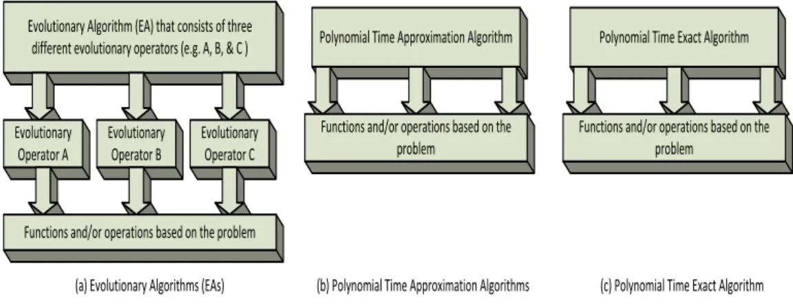
MOSP is an NP-hard problem [8, 3] and its approximate solutions should be determined using heuristics. MOSP problem can be solved using three different types of algorithms:

* Evolutionary Algorithms (EAs)

* Polynomial Time Approximation Algorithms (PTAAs) * Polynomial Time Exact Algorithms (PTEAs)

The EAs mimics the biological process of evolution in search for the optimum solution. First and the most important advantage of solving any multi-objective optimization problems (MOPs) with the EAs is that an EA that is developed to solve any particular MOP remains useful for the other MOPs. The MOPs can be entirely different from each other. The EAs are defined in terms of evolu-tionary operators to produce useful results. The evoluevolu-tionary operators consists of functions or operations that are problem-specific. Therefore, the design of the EA is not dependent on the problem. For instance, Non-dominated sorting genetic algorithm-II (NSGA-II) [4] which is a popular EA was used to solve many MOPs that include: Multi-objective Electromagnetic Optimization [5], Service restoration in distribution systems [6], and optimal application map-ping on NoC infrastructure[7]. Therefore, many problems or different versions

(11)

Evolutionary Algorithm (EA) that consists of three different evolutionary operators (e.g. A, B, & C )

Evolutionary Operator A Evolutionary Operator B Evolutionary Operator C

Functions and/or operations based on the problem

Polynomial Time Approximation Algorithm

Polynomial Time Exact Algorithm

(a) Evolutionary Algorithms (EAs) (b) Polynomial Time Approximation Algorithms (c) Polynomial Time Exact Algorithm

Figure 1.1: Illustration of types of components in EAs, PTAAs and PTEAs of the same problem can be efficiently solved using a same EA. The efforts re-quired to developed optimization algorithms for different problems also reduces significantly. EAs also do not require any pre-computation and calculation in any generation are independent from the previous generations. Therefore, they are robust to dynamic changes in the network.

PTAAs aim to approximately solve the MOSP problem within the bounds of the polynomial amount of time. PTAAs guaranteed to solve any MOP with some solution quality. Most of the PTAAs are described in terms of functions or operations that are based on the problem [8, 9]. Therefore, the FTAAs are specific to one or certain problems. FTAAs require pre-computation of some values. In case of dynamic changes in the network, the computation of the optimal paths should be restarted. Therefore, they are not robust to dynamic changes in the network.

PTEAs are suitable for small size networks only. In huge size networks, their time complexity becomes impractical for most real-time operations. Martin’s algorithm [13] is a PTEA to solve the MOSP problem. The Dijkstra’s Algorithm can solve the shortest path problem in networks and has a time complexity which is better than the other polynomial time exact algorithms. The authors implemented the Dijkstras Algorithm on the nVIDA CUDA graphics processing unit (GPU) and its execution time came out to be around 8 minutes on the road network of the New York City. Gunichev et al. [12] also found the execution time of the Dijkstra’s Algorithm to be eight minutes. Eight minutes is not suitable for most of the real-time operations. Ahn, at al. [14] reported that the time complexity of the Dijkstra’s Algorithm increases with the number of nodes in the network. In huge size networks, Genetic Algorithm (GA) becomes faster than the Dijkstra’s Algorithm.

The structure of the EAs, PTAAs and PTEAs is shown in Fig. 1.1. The EAs comprises of evolutionary operators and therefore, their design is independent from the specific properties of the problem. PTAAs and PTEAs on the other hand, contains functions or operations that are based on the problem and can change from problem to problem.

(12)

Existing Evolutionary Algorithms (EAs) Population-based Algorithms Single-Solution based Algorithms · Memory intensive · Yields good quality solutions · Finds diverse solutions · Specially useful in solving

MOPs with many objectives

· Memory efficient · Require long computation

time. Otherwise, their solution quality is lesser than Population-based algorithms.

Figure 1.2: Illustration of types of EAs

forms. Therefore, the objective functions and constraints can take different forms. MOSP problem also occurs in emerging fields like electric vehicles, where new enhancements are continue to happen. Therefore, the MOSP problem is subject to further modification in the future. The EA approach is specially suitable for such kind of problems because it can incorporate changes in the objective function or constraints without effecting the top-level algorithm. The EA approach also enables that the optimization algorithms to remain useful for the other and unrelated optimization problems.

Many EAs exists to solve the MOPs. The existing EAs can be divided into two types: The first type of EAs works on a single solution and are memory efficient. Simulated Evolution (SimE) and Stochastic Evolution (StocE) [16, 17] are examples of single-solution based EAs. Single solution EAs are suitable for use in embedded systems that have limited memory and computational power. The second type of EAs work on a population of solutions. They are memory intensive but generally yields results better than the single solution based al-gorithms. Genetic Algorithm (GA) [16] is an example of population based EA. This thesis presents two new EAs to solve the MOSP problem. The new EAs aims to be memory-efficient as well as yield quality solutions to the MOSP problem. The two important properties of the proposed algorithms are as fol-lows:

* Memory-efficient than the existing population-based EAs

* Achieves better quality than the existing single-solution based algorithms. The first algorithm is based on Stochastic Evolution (StocE) algorithm. StocE was first proposed by Youssef G. Saab and Vasant B. Rao [17] in 1990 for solving combinatorial optimization problems. StocE algorithm works on a single solution and resembles a biological evolutionary process in which species eliminate some of the bad characteristics of the older generation in order to pro-duce a better new generation. The proposed StocE based algorithm considers

(13)

different sub-paths in a solution as its different characteristics and removes bad sub-paths with new sub-paths from generation to generation.

The second algorithm is an off-spring non-storing GA algorithm. GAs was first proposed by John Holland and his colleagues in the early 1970s [18]. GA simulates the process of natural evolution based on Darwinian principles. The conventional GA algorithms store children chromosomes in the memory and require a total memory of size about twice the population size. The proposed off-spring non-storing GA algorithm, on the other hand, conditionally store children chromosomes in place of the parent chromosome. Therefore, it requires memory almost equal to the size of the population. The memory-efficiency in the proposed algorithms makes them suitable to solve the MOSP problem in embedded systems.

The performances of the proposed algorithms were compared with some famous MOO algorithms: (i) (1-1)-Pareto-Archived Evolution Strategy ((1-1)- PAES) algorithm [20], (ii) Non-dominated Sorting Genetic Algorithm-II (NSGA-II) [4], (iii) Micro-GA [21], (iv) Multi-objective Simulated Annealing (MOSA) [22], and (v) A straight-forward StocE (std-StocE). NSGA-II was suc-cessfully used in many applications like: multi-objective electromagnetic prob-lem that consists of many conflicting objectives [5] and optimization probprob-lem in distribution systems [6]. Micro-GA was also used to solve important problems like optimization problem in Network-on-Chip (NoC) [7]. PAES was also suc-cessfully used to perform optimization required by the AI (artificial intelligence) in video games [23]. The comparison with Std-StocE shows the benefit of using the proposed design of StocE over the standard StocE algorithm.

This dissertation is organized as follows: The second chapter describes some popular multi-objective optimization algorithms. The third chapter describes the MOSP problem in detail and a method of calculating and comparing the performances of different multi-objective optimization algorithms. The fourth chapter contains the description of the proposed algorithms. The fifth and sixth chapters show the application of the proposed algorithms to solve the navigation problem in conventional vehicles and battery electric vehicles. The seventh chapter shows the general forms of the proposed StocE and GA-based algorithms and their comparison with the existing algorithms on several test problems. The eighth chapter discusses the problem of congestion that occurs due to a large number of vehicles and a simple method to minimize the congestion. The last chapter contains the conclusion.

(14)

Chapter 2

Existing Algorithms to

Solve the MOSP Problem

This chapter describes some existing algorithms to solve the MOSP problem. Two types of algorithms are discussed that includes: evolutionary algorithms and polynomial time approximation algorithms.

2.1 Polynomial Time Approximation Algorithms

(PTAAs)

Mandow et al. [9] presented initial results of extending the A* search algorithm to the solution of MOSPs. The new algorithm is named MOA*, which is a heuristic search algorithm used to find non-dominated solutions. The search process in MOA* is guided by heuristic functions. When the guiding heuristic does not meet a certain bounding test, MOA* becomes unreliable and cannot produce any useful solution. However, it is reliable when used with a proper set of heuristics. Tsaggouris and Zaroliagis [10] proposed an improved Fully Poly-nomial Time Approximation Scheme (FPTAS) algorithm for solving MOSPs. Their algorithm resembles the multi-objective Bellman-Ford algorithm. Among FTPASs, it has the best time complexity. Horoba [11] performed an analysis of a simple evolutionary algorithm that consists of a fitness function and mutation operation and found that it met the requirements of a Fully Polynomial Time Randomized Approximation Scheme and its runtime was comparable to that of Tsaggouris and Zaroliagis’s algorithm [10]. The conventional FTPAS requires pre-computation of some values (e.g., node labels which includes cost of links) before determining the optimal path. In case of dynamic changes, the cost of links can change to reflect dynamic changes in the network. Therefore, some or many of the node labels becomes invalid. The conventional FTPAS does not robustly accommodate dynamic changes and the calculation of the shortest path must be restarted several times whenever there are dynamic changes in the network. Because simple EC algorithms perform well and robustly accom-modate dynamic changes in the network, they are often used to solve MOSPs with dynamic changes.

(15)

2.2 Evolutionary Algorithms

Elitist Evolutionary Multi-objective Optimization (EMO) algorithms are the most recent EMOs used for finding Pareto-optimal solutions. In elitist EMO algorithms, good solutions are preserved during iterations. Recent EMO algo-rithms can be classified into two classes: (i) single solution based algoalgo-rithms, and (ii) population based algorithms. The single solution based EMOs work on a single solution and therefore, are quite memory efficient. The population based EMOs work on a population of solutions. They require more memory than the single solution based algorithms but also yield good quality solutions. In this chapter, some popular single solution based and population based algorithms are described.

2.2.1 Single Solution based Algorithms

(1-1)- PAES

Knowles and Corne [20] proposed a multi-objective local search algorithm which they named as: (1-1)-Pareto Archived Evolution Strategy ((1-1)-PAES) algo-rithm. (1-1)-PAES is capable of generating diverse Pareto-optimal solutions. The (1-1)-PAES maintains an archive of Paret-optimal solutions of size m so-lutions. Each solution in the archive has a position in the n-dimensional grid (where n is the number of objectives). The PAES has three portions: (1) the candidate solution generator; (2) the candidate solution acceptance; and (3) the non-dominated-solutions (NDS) archive. The candidate solution generator consists of a simple mutation operation and in each iteration it creates a new solution (called as mutant solution) through performing random mutation in the solution. The design of the candidate solution acceptance function is as follows: If the mutant solution dominates the existing solutions then it is accepted and the current solution is updated. If the mutant solution does not dominate the existing solution then the following rules are applied: If the mutant solution lies in a less crowded region of the archive then the existing solution is updated to the mutant solution. The NDS archive of m solutions is maintained. However, when the archive becomes full then the following method is used to remove a solution from the archive to make space for the new solution (c). The grid po-sition of c in the archive is determined. If c lies in a less crowded region than any solution in the archive of pareto-optimal solutions then a solution that lies in the most crowded region is removed and c is inserted to the archive. The ex-perimental results show that despite being simple, it is very effective in solving multi-objective optimization problems.

MOSA

Smith, et al. [22] proposed a multi-objective simulated annealing (MOSA) al-gorithm. The algorithm keeps an archive of pareto-optimal solutions. They proposed a transformation function to transform a multi-objective solution into an energy value. A solution can be compared with another solution based on its energy value and a solution can be better, equal or worse than the other solution. The energy of any solution is determined by calculating the number of solutions in the archive of pareto-optimal set that dominates it. Therefore, the solutions having higher energy values are considered inferior. All solutions

(16)

in the archive of pareto-optimal solutions are mutually non-dominating. A new solution is accepted to replace the existing solution according to an exponential equation of energy difference. When the archive of pareto-optimal solutions contains too few solutions then the efficiency of the energy difference equation becomes low; therefore, new solutions (real and/or artificial) are considered to be a part of the archive of pareto-optimal solutions. Two methods can be used to increase the number of solutions in the archive of pareto-optimal solutions: (i) Conditional removal of the dominated solutions from the archive, and (ii) Creation of artificial solutions through linear interpolation. In the first method, the dominated solutions whose removal reduces the size of archive below some specified limit are retained in the archive. In the second method, linear interpo-lation is used to generate new points. The new hypothetical points are evenly spread along the pareto-optimal front and dominated by at-least one actual solution in the archive of the pareto-optimal solutions.

2.2.2 Population based Algorithms

Genetic Algorithm (GA) is a famous population based algorithm. This section shows some famous variants of GA to solve the MOO problem.

Micro-GA

Coello and Pulido [21] proposed Micro-GA for high quality multi-objective op-timization. It stores solutions in two types of memories. The first type is the population memory and the second type is an external memory to store pareto-optimal solutions. The population memory is further divided into a replaceable portion and a non-replaceable portion. The replaceable portion contains the so-lutions that can be altered during the optimization; whereas, the non-replaceable portion contains the solutions that cannot be changed after being initialized in the initialization step. The Micro-GA contains a micro-GA cycle that works on a separate population of solutions in which the elements are selected from the replaceable and non-replaceable portions of the population memory. The micro-GA cycle consists of the conventional GA operators (crossover and mu-tation) and executes for a smaller number of iterations. When the micro-GA cycle finishes, up to two new pareto optimal solutions are copied from its popu-lation to the replaceable portion of the popupopu-lation memory and to the external archive of pareto-optimal solutions. In the next micro-GA cycle, the elements of the population of the micro-GA cycle are again selected from the population memory. When the stopping criteria of the Micro-GA is reached then algorithm goes to the termination instead of initiating another micro-GA cycle.

NSGA-II

Deb, et al. [4] proposed Non-dominated Sorting Genetic Algorithm-II (NSGA-II) to perform multi-objective optimization. NSGA-II has low computational complexity. During its iterations, it preserves two types of solutions: non-dominated solutions and solutions that are most distinct in the population. By doing so, the algorithm maintains both quality and diversity among its solutions. An iteration cycle consists of the following steps: (i) The population (includ-ing children chromosomes) is sorted accord(includ-ing to the non-domination count of

(17)

the solutions. The chromosomes are assigned pareto front values such that the non-dominated solutions are selected in the first front. The solutions that are non-dominated after removing the chromosomes of the first front are placed in the second front. The pareto-front values to the remaining solutions are also assigned in the same way. (ii) The crowding distances of the chromosomes are calculated based on the distances between the objective function values of the chromosomes. The crowding distance helps in developing a uniformly spread pareto optimal front. (iii) The chromosomes for the population of the next iter-ation are selected from the combined populiter-ation (i.e., populiter-ation and children chromosomes). The solutions having lesser pareto-front values are first selected and the solutions of the last front are selected based on the crowding distance. The children chromosomes are created using crossover and mutation operations. Experimental results have shown that this algorithm is very successful in finding diverse Pareto-optimal sets of solutions for multi-objective optimization prob-lems. Bora, et al. [24] added greedy reinforcement learning to NSGA-II for self-tuning its parameters. Their new algorithm, RL, tunes four NSGA-II parameters—the probabilities of crossover and mutation operations and the distribution indices in crossover and mutation operations—on the basis of the results of previous generations. NSGA-RL is slower than NSGA-II; however, its results are closer to the NSGA-II results that have the best possible parameter values.

(18)

Chapter 3

Problem Description and

Performance Measurement

This chapter describes the MOSP problem in detail. It also describes the meth-ods of measuring the solution of different algorithms. The result of any MOSP problem is a set of pareto-optimal solutions. The quality of the pareto-optimal solutions obtained by different algorithm can vary, therefore, calculating the performance of the pareto-optimal sets is important.

3.1 Problem Description

Let us consider an undirected graph G(V, E), where V is the set of all vertices in the network and E is the set of all edges in the network. An edge ex∈ E has

a starting node and an ending node. For any edge ei, the starting node is

rep-resented as ei.st and the ending node is represented as ei.en, where st, en ∈ V .

Any edge ei∈ E has up to K weights associated with it, which are represented

as {ei.w1, ei.w2, ..., ei.wK}. The weights of the edges should be non-negative

real numbers. One or more point-to-point (P2P) paths exist between the nodes in the graph. If s and d (where s, d ∈ V ) are two distinct nodes in G, which are selected as the source and destination nodes. Then many paths exist between s and d. A path is represented by P and is a sub-set of E, i.e., P ⊆ E. If ex

is the first edge in P and ey is the last edge in P , then ex.st should be s and

ey.en should be d. For any two consecutive edges em and en edges in P (s.t.,

en lies after em in P ), em.en = en.st.

In the multi-objective shortest path problem (MOSP), the path P is asso-ciated with up to K1 (where 1 < K1 ≤ K ) objective functions and up to K2

constraints (where 0 ≤ K2 ≤ K). The objective functions can be represented

as f1, f2, ..., fK. The value of any objective function can be calculated as:

fk(P ) =

X

ex∈P

ex.wk, for k= 1 to K1 (3.1)

The set of constraints are represented as g1(P ), g2(P ), ..., gM(P ). The value of

any constraint gk(P ) can be determined as:

gk(P ) =

X

ex∈P

(19)

The MOSP problem can be defined as:

M inimize(f1(P ), f2(P ), ..., fk(P )), s.t., {g1(P ), g2(P ), ..., gk(P )} can be satisfied.

(3.3) The objective functions and constraints can have any other form based on the actual problem. When the number of objectives is greater than one, i.e., K1 > 1 and K > 1, then the MOSP problem becomes an NP-hard problem

[8, 3] and heuristics should be used to solve it. The multiple objectives can be in contradiction to each other and no single solution is said to be optimum in all objectives. Therefore, a set of pareto-optimal solutions should be obtained for the MOSP problem. A pareto-optimal set contains all solutions that are not dominated by any other solution. A solution A dominates another solution B (which is represented as A B), if A is better than B in at-least one objective function value and A is not inferior than B in any objective function value.

3.2 Performance Measurement

EAs are used to approximately solve the multi-objective optimization problems. Therefore, the quality of pareto-optimal set obtained from any EA should be calculated. Hypervolume (HV) metric [25, 26] is a popular method for finding and comparing the quality of pareto-optimal solutions obtained from different algorithms. The HV metric calculates the space covered by the solutions in the pareto-optimal set of any algorithm in the solution space. The HV indicator measures both quality and diversity of solutions. The algorithms that yield higher values of the HV metric are considered good. The choice of performance metric depends on the information available about the problem. Many test problems were designed to do experiments with the multi-objective optimiza-tion algorithms. In actual or true pareto-front of the test problems is known. Therefore, many performance metrics exist for the test problems. The real-world problems, on the other hand have unknown true pareto-fronts. Therefore, very few performance metrics exist for real-world problems. HV metric has the ad-vantage that it can works well in problems with unknown true pareto-front.

The HV metric is illustrated in Fig. 3.1 for a minimization problem of two objectives. In Fig. 3.1, the pareto-optimal set has two solution a1 and a2 and b

is the maximum bounding point. The shaded portion shows the HV value of the pareto-optimal set. The bounding point (b) has coordinates equal to the number of objectives in the multi-objective problem. The value of b can be determined by using the method proposed by Knowles [27]. He selected the bounding point as bj= maxj+δ(maxj−minj), where bjis the bounding value of the jthcoordinate

and maxj and minj are the maximum and minimum values, respectively, of the

jth _{coordinate in the Pareto-optimal solutions. The value of δ can be taken as}

0.01. The HV of the Pareto-optimal sets were calculated using the tool proposed by Fonseca, et al. [28]. The tool uses an improved version of the Hypervolume by Slicing Objectives algorithm [29], which accurately computes the HV. This algorithm is among the fastest methods to compute HV.

When two algorithms (A and B) are compared against each other. If HVA

is the HV of algorithm A and HVB is the HV of the algorithm B. The ratio

HVA

HVB has value equal to greater than 1 when HVA≥ HVB. The ratio can relate

(20)

Space covered by the pareto-optimal solutions f1(P) f2(P) a1 a2 b

Figure 3.1: Illustration of the HV metric. Table 3.1: Details of the Road Networks

Road Network Description Number of nodes Number of edges

BAY Road network of the San Francisco Bay Area 321,270 800,172

COL Road network of the Colorado state 435,666 1,057,066

NY Road network of the New York City 264,346 733,846

Table 3.2: Variables representing the HV of the algorithms

Symbols Description

HVStocE HV of the Proposed StocE-based algorithm

HVGA HV of the Proposed Off-Spring Non-Storing GA algorithm

HVN SGA−II HV of the existing NSGA-II algorithm

HVM icro−GA HV of the existing Micro-GA algorithm

HVP AES HV of the existing PAES algorithm

HVM OSA HV of the existing MOSA algorithm

HVStd−StocE HV of the straight-forward StocE algorithm

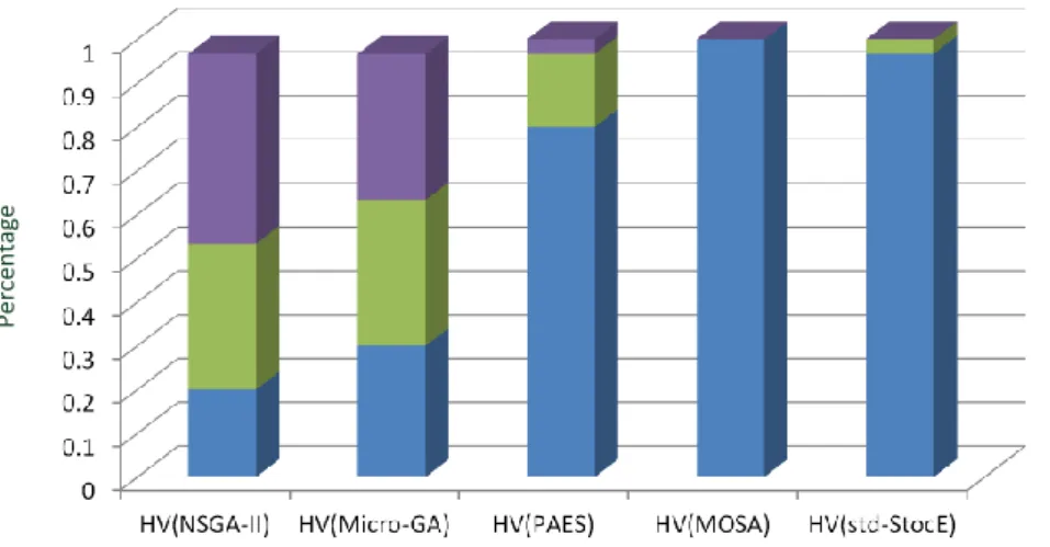
HV (N SGA − II) Ratio of the HV of the Proposed algorithm to that of the NSGA-II HV (M icro − GA) Ratio of the HV of the Proposed algorithm to that of the Micro-GA HV (P AES) Ratio of the HV of the Proposed algorithm to that of the PAES HV (M OSA) Ratio of the HV of the Proposed algorithm to that of the MOSA HV (Std − StocE) Ratio of the HV of the Proposed algorithm to that of the std-StocE

and B represents any of the existing algorithm. Then, the ratio HVA

HVB gives the

following information: (i) If HVA

HVB ≥ 1, then the proposed algorithm is equal

to or better than the existing algorithm, (ii) If HVA

HVB = x < 1, then the HV of

the proposed algorithm is about x% of the existing algorithm. When x value is closer to 1 like 0.9, 0.8 or 0.7 then the performance of the two algorithms is considered to be very close.

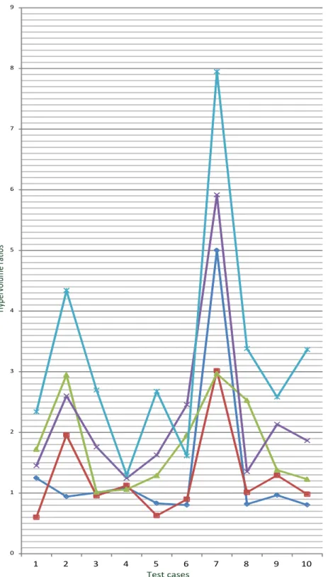
The MOSP problem is solved on the road networks of some cities and states of the United States of America. The DIMACS design challenge website [30] contains huge size road networks of some cities and states of United States of America. The selected road networks are shown in Table 3.1. Table 3.1 shows the symbol, description of the road network and the number of nodes and edges that it contains. All the road networks are of huge sizes. An experiment consists

(21)

of randomly selecting the source and destination nodes in the road network and finding MOSPs between them. The EAs are non-deterministic algorithms and they yield a different solution every time. Therefore, a test-case consists of up-to five trials of an experiment. The average HV of the five trials is the HV of that test-case. This works consists of two proposed algorithms and five existing algorithms. The symbols used to represent the HV of a test-case (i.e., average HV of its five trails) of different algorithms is shown in Table 3.2. In the ratios of the HVs, the numerator contains the HV of the proposed algorithm. The proposed algorithm refers either to the Proposed StocE-based algorithm or Proposed Off-spring Non-storing GA-based algorithm based on the context. in the ratios HVN SGA−II, HVM icro−GA, HVP AES, HVM OSA, and HVStd−StocE,

when their value is greater than 1, then the proposed algorithm performs better than the existing algorithm. When their value is 1, then the proposed and the existing algorithm performs equal to each other. When their value is lesser than 1, then the existing algorithm performs better than the proposed algorithm.

(22)

Chapter 4

Proposed Algorithms

This section describes two new EAs for solving the MOSP problem. Our first proposed algorithm is based on Stochastic Evolution (StocE); and our second algorithm is based on Genetic Algorithm (GA).

4.1 Method to generate a random paths

In the proposed algorithms, a random path needs to be built between any source and destination nodes in the network. Fig. 4.1 shows a method to generate a random path between the nodes s and d. The method can be invoked by calling the function f orm path(s, d) . The first four lines initialize the variables. Each node has two attributes π and sel associated with it, π is used to store the node that is preceding it in the path from source to destination and sel is used to indicate that the corresponding node is entered in the queue Q at least once. The while loop between lines 6 and 15, retrieves an element from Q i.e. η then inspects the nodes that are adjacent to η and inserts new elements in Q according to the conditions shown. The second while loop between 17 and 20, forms a complete path between the source and destination node by following the π attribute of the nodes. Reverse Order function in line 21, corrects the order to path from source to destination.

4.2 Proposed StocE based Algorithm

StocE is a general purpose iterative stochastic algorithm [16, 17]. It resembles a biological evolutionary process in which the solution eliminates its bad char-acteristics from generation to generation. The perturb operation in the StocE performs the task of elimination of the bad characteristics from the solution. This paper proposes a StocE algorithm for the MOSP problem. In the pro-posed algorithm, sub-paths in the solution are considered as its characteristics and the solution replaces the bad sub-paths with better sub-paths from gen-eration to gengen-eration. The proposed StocE based algorithm is shown in Fig. 4.2. The inputs are: source and destination nodes (s & d); iter, which is the maximum number of iterations in the Perturb-cycle; mt, which is the maximum

iteration in the Mutation-cycle; N um, which is the number of sub-paths (i.e. the number of characteristics) to be considered in the Perturb operation; Pb,

(23)

Input: nodes: s, & d

Output: y: A path from s to d

nodes.-1: Q= ∅, done= 0, y =∅

2: for (each node ni∈ V ) do

3: ni.sel= false, ni.π= 0

4: end for

5: Q = Q ∪ {s}

6: while (!done) do

7: η= A randomly selected element from Q, Q = Q − {η}

8: for (each node nx∈ Adj(η)) do

9: if (nx== d) then

10: nx.π = η, done = 1

11: else if (!nx.sel and Q ∩ {nx} == ∅ ) then

12: nx.π = η, Q = Q ∪ {nx}, nx.sel = true 13: end if 14: end for 15: end while 16: n = d, y = y ∪ {n} 17: while (n! = src) do 18: n = n.π 19: y = y ∪ {n} 20: end while 21: Reverse Order(y) 22: return y

(24)

(25)

which is the probability value used in the Perturb operation; and m is the max-imum number of solutions in the archive of pareto-optimal solutions. The value of Pbshould be kept large, (e.g. 0.7). The first step is initialization in which the

solution S is initialized with a random solution or path between the nodes s and d. The random path can be built using the function f orm path. A loop which contains two cycles (i.e. Perturb-cycle and Mutation-cycle) starts after the ini-tialization step. The Perturb-cycle creates new solutions through the perturb operation and store the new solutions in the set SA. The set SA is initialized to null at the start of the Perturb-cycle and stores all solutions created through the perturb operation. After the completion of the Perturb-cycle, the function str optimal() is called. Using the str optimal() function, the solutions in SA that are not dominated by any other solution in both sets P S (where P S is the archive of pareto-optimal solutions) and SA are inserted into P S. The mu-tation cycle also contains up to mt number of iterations. The Mutation-cycle

contains small number of cycles so as to increase the possibility that the mutant solution dominates (i.e. better than) the existing solution and also the mutation cycle should not consume much execution time. Due to the mutation operation, the next iteration of the outer-most loop executes on a different solution then the previous iteration. The stopping criterion can be the maximum number of iterations or maximum execution time. After stopping criteria is reached, the solutions in P S are returned by the algorithm. The different steps are described in detail in the following sub-sections.

4.2.1 Perturb Operation

In StocE, each characteristic of the solution should prove its suitability to remain in the next generation. The perturb operation implements this feature of the StocE. This work considers different sub-paths in the solution as its characteristics. Therefore, the sub-paths should calculate their suitability to remain in the next generation. Fig. 4.2 shows that the Perturb cycle has iter number of iterations. In each iteration, the Perturb operation is applied to form a new solution S0 from S. S0 is stored in SA and at the end of the Perturb cycle, up to iter number of solutions are stored in SA.

The proposed perturb operation consists of two parts. The first part consists of finding a sub-path in S which is minimally suitable to remain in the next generation. The suitability of any sub-path (p) is determined based on two values: (i) the values of its objective function values (f1(p), f2(p), ..., fK(p)),

and (ii) the number of elements in the sub-path. The sub-paths that have higher values of the objective functions and lesser elements are considered to be less suitable for the next generation. The second part consists of finding an alternative sub-path to replace the selected sub-path from S. Alternative sub-path replaces the selected sub-path if it dominates the selected sub-path, or is better than the selected sub-path in any objective function value.

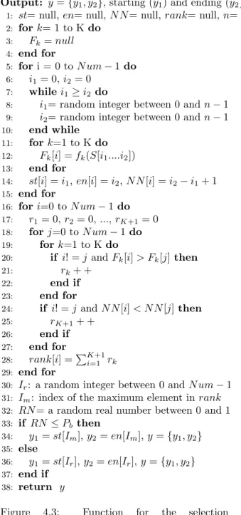
Fig. 4.3 shows the first part of the perturb operation and Fig. 4.4 shows the second part of the perturb operation. Fig. 4.3 shows the select subpath() function, the inputs are the current solution S, positive integer (N um), and a positive real number (Pb). The N um is used to specify the number of sub-paths

to be considered in the current solution. The f or loop between lines 5 and 15 stores the starting and ending nodes of the selected sub-paths in the arrays st and en. N N stores the number of nodes in each sub-path. The f or loop

(26)

Input: S: current solution, N um ∈ Z+, Pb∈ R+, P b ∈ {0 ≤ P b ≤ 1}

Output: y = {y1, y2}, starting (y1) and ending (y2) indices of a sub-path in S

1: st= null, en= null, N N = null, rank= null, n= number of elements in S

2: for k= 1 to K do 3: Fk = null 4: end for 5: for i = 0 to N um − 1 do 6: i1= 0, i2= 0 7: while i1≥ i2 do

8: i1= random integer between 0 and n − 1

9: i2= random integer between 0 and n − 1

10: end while

11: for k=1 to K do

12: Fk[i] = fk(S[i1....i2])

13: end for

14: st[i] = i1, en[i] = i2, N N [i] = i2− i1+ 1

15: end for

16: for i=0 to N um − 1 do

17: r1= 0, r2= 0, ..., rK+1= 0

18: for j=0 to N um − 1 do

19: for k=1 to K do

20: if i! = j and Fk[i] > Fk[j] then

21: rk+ +

22: end if

23: end for

24: if i! = j and N N [i] < N N [j] then

25: rK+1+ + 26: end if 27: end for 28: rank[i] =PK+1 i=1 rk 29: end for

30: Ir: a random integer between 0 and N um − 1

31: Im: index of the maximum element in rank

32: RN = a random real number between 0 and 1 33: if RN ≤ Pb then 34: y1= st[Im], y2= en[Im], y = {y1, y2} 35: else 36: y1= st[Ir], y2= en[Ir], y = {y1, y2} 37: end if 38: return y

Figure 4.3: Function for the selection of a sub-path y = select subpath(S, N um, Pb).

(27)

Input: S: current solution, N um ∈ Z+_{, P}

b ∈ R+, P b ∈ {0 ≤ P b ≤ 1},

G = (V, E)

Output: S: solution after the perturb operation

1: I = {i1, i2} = select subpath(S, N um)

2: e1= (na, nb) = S[i1], e2= (nc, nd) = S[i2]

3: t = f orm path(na, nd)

4: S0= Concatenate{S[0...i1− 1], t, S[i2+ 1....]}

5: return S0

Figure 4.4: Proposed Perturb operation S0 = P erturb(S, N um, Pb).

between lines 16 and 29 finds the ranks of all sub-paths. The sub-paths that are less suitable are assigned higher rank values. The sub-paths that have higher objective function values and lesser number of nodes are assigned higher ranks. In line 30, Im is the index of the sub-path that has the highest rank value.

In line 31, Ir is the index of a randomly selected sub-path. In lines 33 to 37,

the starting and ending indices of the sub-path that has maximum rank value is stored in y1 with probability Pb. With probability 1 − Pb, the starting and

ending indices of a random sub-path is stored in y1. The Pbis assigned a higher

value, therefore, generally the algorithm in Fig. 4.3 returns a sub-path that is least suitable to be kept in the next iteration as compared to the several other randomly selected sub-paths.

Fig. 4.4 shows the second part of the perturb operation. The inputs are the current solution (S), N um and Pb, which are already described. The function

returns a new solution which is obtained after applying the perturb operation. In line 1, a sub-path is chosen in S by calling the function select subpath(). e1

and e2 represent the edges that contains the starting and ending nodes of the

sub-path. In line 3, a new sub-path t is formed between the starting (na) and

ending nodes (nb) of the selected sub-path. In line 4, a new path S0by inserting

t between the upper and lower portions of the current solution. In lines 5 and 6, S is updated to S0, if S0 is not dominated by S or S0 is better than S in any objective function value.

4.2.2 Mutation

Input: S: current solution, d destination node Output: S0_{: solution after the mutation operation}

1: n= number of elements in S, S0 _{= S}

2: rn= random integer between 0 and n − 1

3: ern= (na, nb)= S 0_[r n] 4: t = f orm path(na, d) 5: S0= concatenate{S0[0...rn− 1], t} 6: return S0

Figure 4.5: Mutation Operation.

Fig. 4.2 shows the Mutation-cycle that comprises of up to mtnumber of

it-erations. The Mutation-cycle aims to find a new solution through mutation that dominates the existing solution. However, after mtiterations are completed and

(28)

no new solution can dominate the existing solution, then the existing solution is updated to the solution that is created in the last iteration of the Mutation-cycle. The purpose of the mutation operation is to move the current solution to another random location in the solution space. This operations aims to in-crease the diversity of solutions and escaping from local minima. The mutation operation is shown in Fig. 4.5. It first selects a random edge ern in the current

solution, then forms a new random path from the starting node (i.e. na) of

selected edge to the destination node (d). The mutant solution S0 is returned at the end.

4.2.3 Store pareto-optimal solutions

Fig. 4.2 shows that the function str optimal() is executed after the completion of the Perturb-cycle. Using the function str optimal(), the solutions in the set SA are stored in the archive of pareto-optimal solutions (i.e., P S) if they are feasible as well as not dominated by any other solution in the sets SA or P S. The solutions in SA are inserted into P S one by one. The solution from SA is compared with the solutions that already exist in SA. If the solution from SA is feasible and not dominated by any solution in P S, then it is inserted into P S. The solutions in P S that are dominated by the solution from SA are removed from P S. The maximum size of the archive of the pareto-optimal solutions (P S) is m solutions. When the archive becomes full, then one of the following two approaches can be used to replace an existing solution with the new solution in the archive of pareto-optimal solutions. The first approach is to randomly select a solution in the archive and replace it with the new solution. The second approach is the adaptive grid method proposed by Knowles, at al. [20]. It is used to decide if the solution should be accepted by replacing another already existing member of the archive. In this method, each solution in the pareto-optimal archive has a grid location. If the new solution lies in a less crowded location in the grid, then it is accepted in place of a solution that lies in a crowded location of the grid. The grid has dimensions equal to the number of objectives, and the range of each dimension is known from the solutions in the archive. The grid location of any solution is determined by recursively bisecting each dimension and finding the half in which the solution lies. The maximum number of sub-divisions in each dimension is set by the user and an example value is 15 or 25.

4.3 Proposed Off-Storing Non-Storing GA

The GA and its different variants (like NSGA-II, Micro-GA, etc) create children chromosomes equal to the size of the population. Therefore, if the population size is N1, then the GA stores a total of 2 × N1 solutions in the population.

In our proposed GA-based algorithm, a child chromosome after its creation through the crossover or mutation operation is not stored at a new memory location but conditionally stored at the place of its parent chromosome. The child chromosome replaces its parent chromosome under the following condi-tions: (i) If the child chromosome dominates the parent chromosome, (ii) If the parent chromosome is not pareto-optimal solution in the existing population then the child chromosome always replaces its parent chromosome. Therefore,

(29)

additional amount of memory is not required to store the children chromosomes. The algorithm consists of two GA operations: crossover and mutation. In each iteration, all chromosomes undergo any one GA operation. Dominated chromo-somes prefer the crossover operation and non-dominated chromochromo-somes prefer the mutation operation. The second parent in the crossover operation is al-ways a non-dominated chromosome that has some common genes with the first parent. The first parent in the crossover operation is considered as the actual parent chromosome.

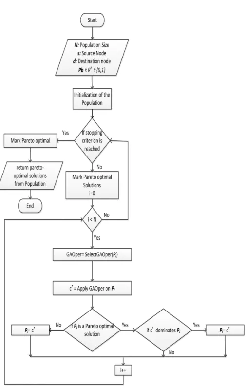
The proposed GA-based algorithm is shown in Fig. 4.6. The inputs to the algorithm are: Population size (N ), source and destination nodes (s and d), a probability (Pb) which is used in selecting a GA operator for the chromosome.

The first step is initialization. After initialization, the outer-most loop performs the optimization until the stopping criterion which can be the maximum number of iterations or maximum execution time is reached. In the optimization, the first step is to mark the chromosomes in the population that are pareto-optimal and feasible in the current population. In that way, the pareto-optimal solutions can be preserved in the GA operations. The next step consists of a loop that has N iterations. In any iteration, Pi represents the chromosome that exists

at the ith _{position in the Population. First, a GA operator is selected for the}

chromosome Pi and then the selected GA operator is applied to Pi. The new

chromosome that is created after applying the GA operator is called c0. If Pi

is a non-dominated chromosome and c0 dominates Pi then the existing value

of Pi is replaced by c0. If Pi is a not a non-dominated chromosome then c0

replaces the existing value of Pi. After the stopping criterion is reached, then

the pareto-optimal and feasible solutions in the Population are returned by the algorithm. The remaining part of this section describes the main operations in the proposed algorithm.

4.3.1 Initialization

In this step, the Population is initialized with up to N distinct and random chromosomes. Each chromosome is a complete solution or path between the nodes s and d. The random paths are generated using the function f orm path().

4.3.2 Mark Pareto-Optimal Solutions

The chromosomes are associated with an attribute sel which is initially set to the false value. When its value is true then the chromosome is called as selected. In this step, all chromosomes in the Population that are feasible as well as not dominated by any other solution in the Population are selected and the values of their sel attributes are set to true.

4.3.3 Selection of the GA Operation

The proposed algorithm contains a set of GA operations, which is represented as GAset. The set consists of two elements, i.e., GAset= {Crossover, M utation}.

All chromosomes must go through any one of the operations from the set GAset.

The crossover operation requires that a common node should exist between the two parents [14]. In a conventional GA, parents are selected by methods such as roulette-wheel or tournament selection. This work proposes that the crossover

(30)

(31)

Input: Pi∈ P opulation, s: source node, P opulation

Output: y=1, if Pi has a feasible pair in P opulation. .

1: cnt=0

2: for each chromosome Pj∈ P opulation and Pi6= Pj do

3: for each edge ex= (na, nb) ∈ Pj do

4: for each edge ey= (nu, nv) ∈ Pi do

5: if na== nu6= s then

6: cnt++

7: Exit from the nested f or loops

8: end if 9: end for 10: end for 11: end for 12: if cnt > 0 then 13: return 1 14: else 15: return 0 16: end if

Figure 4.7: Method used to find if Pi has a feasible pair in the population

y = CheckCn(Pi, P opulation, s).

operation can be applied to any chromosome Pi such that the second parent is

any feasible pair for Pi. A feasible pair for Pi is a non-dominated chromosome

that has at least one common node with Pi (excluding source and destination

nodes). The procedure to check if any feasible pair exists for a chromosome Piis

shown in Fig. 4.7 and is represented as CheckCn(). The function CheckCn(Pi)

returns 1 if at least one pair exists for Pi, otherwise it returns 0.

The method to select a GA operation for the chromosome is shown in Fig. 4.8. The basic idea behind the proposed assignment of GA operations is the following. The chromosomes are distinguished into two classes: non-dominated and dominated. The crossover operation is selected for the dominated chromo-somes with a high probability (Pb). As previously mentioned, the second parent

in the crossover operation should be a non-dominated chromosome. Therefore, the dominated chromosomes have a high probability of producing a better off-spring by exchanging genes with a non-dominated chromosome. On the other hand, a mutation operation is selected for the non-dominated chromosomes with a higher probability (Pb) so that they try to produce a better quality offspring

by introducing new genes. The inputs to the method in Fig. 4.8 are as follows: chromosomes Pj and Pb which is a real number between 0.5 and 1. At the end

of the method, a GA operation is selected for the input chromosome Pj.

4.3.4 GA Operations

GAset in the proposed algorithm consists of two operations: crossover and

mu-tation. Therefore, GAset = {crossover, mutation} and new operations can be

added into the set GAset at any time. The function SelectOperation() should

be modified if new operations are added into GAset. The next two subsections

(32)

Input: Pj∈ P opulation, Pb∈ {x ∈ R|0.5 < x ≤ 1}

Output: OP ER : A GA operation for Pj

1: v= CheckCn(Pj)

2: r: random real number between [0, 1]

3: if v == 0 then

4: return Mutation

5: else if Pj.sel == true and r ≤ Pb then

6: return Mutation

7: else if Pj.sel == true then

8: return Crossover 9: else if r ≤ Pb then 10: return Crossover 11: else 12: return Mutation 13: end if

Figure 4.8: Method used to select a GA operation for the chromosome Pj,

OP ER = SelectOperation(Pj).

Input: Pj, P opulation, s: source node

Output: Index of the feasible pair

1: for each particle Pk∈ P opulation do

2: if Pk.marked == true and Pj6= Pk then

4: for each edge ey= (nu, nv) ∈ Pk do

5: if na== nu6= s then

6: I= index of Pk in the P opulation

7: Pc= Pc∪ I

8: exit to the outermost for loop

9: end if

10: end for

11: end for

12: end if

13: end for

14: selP = randomly select an element from Pc

15: return selP

Figure 4.9: Procedure to select a feasible pair for Pj, i.e., y =

(33)

Input: Pj, P opulation.

Output: c0: offspring

1: c0= P opulation[f indgbest(Pj)]

2: Cn = null

4: for each edge ey= (nu, nv) ∈ c0 do

5: if (na== nu) then

6: Cn= Cn∪ na

7: end if

8: end for

9: end for

10: r= a randomly selected node from Cn

11: c0= concatenate(c0(s..., r), Pj(r, ....d))

12: return (c0)

Figure 4.10: Procedure to apply the crossover operation to particle Pj, i.e.,

c0= Crossover(Pj, P opulation)

Input: Pj∈ P opulation, d: destination node

Output: c0: offspring

1: er= (na, nb): a randomly selected edge in Pj

2: c0= f orm path(na, d)

3: c0= concatenate(Pj(e0, ..., ex), c0) (s.t. ex= (nx, na))

4: return (c0)

(34)

Table 4.1: Memory requirements of the algorithms

Component Number of Paths in different Algorithms

Prop. StocE Prop. GA NSGA-II Micro-GA (1-1)-PAES MOSA

Population 1 N N N 1 1

Children 1 1 N N 1 1

Pareto-optimal set m 0 0 0 m m

others iter 0 0 m1 0 0

total paths 2 + iter + m N + 1 2N 2N + m1 2 + m 2 + m

4.3.5 Crossover Operation

The crossover operation in this algorithm is different from conventional single-point crossover. Before the crossover operation can be applied on the chromo-some Pj ∈ P opulation, the second parent should be determined by calling the

function f indpair(Pj), which is shown in Fig. 4.9. The procedure finds a

feasi-ble pair for Pj. As shown in Fig. 4.9, the indexes of all feasible pairs for Pj are

stored in Pc. Then, an element is randomly selected from Pc and is returned.

The crossover operation which is quite similar to the one proposed by Ahn, et al. [14] is shown in Fig. 4.10. The crossover operation stores the second parent in variable c0. The common nodes between C and Pj are stored in Cn. Then,

an element is randomly selected from Cn. In the second to last row, c0is formed

by combining the upper portion of c0 _{with the lower portion of P}

j. Finally, c0 is

returned

4.3.6 Mutation Operation

The proposed mutation operation is shown in Fig. 4.11. The inputs are: a chromosome Pj and destination node d. An edge is randomly selected in Pj

that is represented as er= (na, nb), where naand nb are its starting and ending

nodes. Then a random sub-path is formed between the nodes na and d. In the

next step, c0 is updated to store the newly created path between the nodes s and d.

4.4 Estimation of the Memory Requirements

This section presents an estimation of the memory requirements of the pro-posed algorithms in terms of maximum number of solutions which they store in the memory at any time during their execution. For comparison purposes, the memory required by some famous multi-objective optimization algorithms including NSGA-II, Micro-GA, (1-1)-PAES and MOSA are also shown.

The memory requirements in terms of the number of paths that should be stored in the memory by the algorithms are shown in Table 4.1. The first col-umn mentions the component of the algorithm that store the specified number of paths; the second column mentions the number of paths for different algo-rithms. The “Prop.” acts as short form of “Proposed”. The number of paths are calculated based on the input parameters of the algorithms. In that way, different input parameters have different memory requirements. The descrip-tion of values in the first column are as follows: (i) “Populadescrip-tion” refers to the population of solutions in the algorithms; (ii) “Children” refers to the number of chromosomes which are created through the GA operators (crossover and/or

(35)

Table 4.2: Memory requirements based on typical values

Algorithm Parameter values Number of Paths

Proposed StocE m = 10, iter = 3 15

Proposed GA N = 20 21

NSGA-II N = 20 40

Micro-GA N = 10, m1= 20 40

(1-1)-PAES m = 10 12

MOSA m = 10 12

mutation); (iii) “Pareto-optimal set” mentions the size of the pareto-optimal set; (iv) “others” include the number of paths to be stored in the memory by the remaining components of the algorithm. In the proposed StocE based algo-rithm, “others” include number of paths to be stored in the Perturb cycle. In the Micro-GA algorithm, “others” include the paths that needs to be stored in the memory by the replaceable and non-replaceable memories and their value is represented as m1. .

4.5 Comparison of Memory Requirements with

Some Typical Values

This section shows the comparison of the memory requirements of the proposed algorithms with the existing algorithms. The authors of NSGA-II used a popu-lation size of 20 [4] in their experiments. Therefore, the typical values of param-eters have a population size of 20. The experiments in the next three chapters use the same parameter values to solve the vehicles’ navigation problem. The typical values are selected such that the population size in all population-based algorithms is same. The NSGA-II and Micro-GA require additional memory to store the children chromosomes, therefore, their overall memory requirement is higher than the proposed algorithms.

In Table 4.2, the first column mentions the algorithm. The second column mentions parameter values that are relevant with respect to determining the memory requirements. The last column mentions the memory requirements of the algorithms in terms of the number of paths. The results show that the proposed algorithms are memory-efficient than the existing population based multi-objective algorithms. The solution quality of the algorithms will be shown in the next two chapters. The next chapters show that based on typical values The memory requirement of an algorithm should be combined by its solutions quality The solution quality will be analysed in the next two chapters.

4.6 Summary

This chapter presents two new EAs to solve the MOSP problem. The first algorithm is based on StocE algorithm and treats the random sub-paths in a solution as its characteristics. During optimization it replaces the bad sub-paths with good sub-paths. The second algorithm is an Off-Spring Non-Storing GA. The GA generally creates children chromosomes equal to the population size. The proposed GA is different from the conventional GA because it minimizes the memory requirements of the algorithm by not storing children chromosomes. The children chromosomes either replace their parent chromosomes or being

(36)

dis-carded soon after their creation. An estimation and comparison of the memory requirements of the proposed algorithms with the existing algorithms shows that the proposed algorithm uses lesser memory than the famous population-based algorithms.

(37)

Chapter 5

Application of the Proposed

Algorithms to the Vehicle

Navigation Problem of

Conventional Vehicles

5.1 Introduction

This chapter shows the application of the proposed algorithms to solve the navigation problem of internal combustion engine based vehicles (ICEVs). The navigation problem in ICEVs aims to find one or more point-to-point (P2P) MOSPs in a road network. The objectives in the MOSP problem are generally minimizing the length of the paths and the travelling time on the paths. The length of a path is equal to the sum of the lengths of the individual edges that are included in it and is generally expressed in km. The travelling time on a path is based on many factors such as the traffic, condition of the roads, road width, maximum allowed speed of the vehicles, etc. The travelling time is generally not related with just length of the path. Therefore, length of the path and their travelling time can be in contradiction to each other. Therefore, a set of pareto-optimal solution should be determined for the MOSP problem for ICEVs.

Let us consider a road network G = (V, E), where V contains all intersections in the road network and E contains all roads that join the intersections in the road network. Any edge ei ∈ E has a starting node u and an ending node v

and is associated with up to two attributes ei.l and ei.SA. ei.l represents the

length of the edge and ei.SA represents the average travelling time on the edge

for the ICEVs vehicles. The driver selects two distinct nodes s and d in the road network and wants to find one or more paths from s to d. If P represents a path between nodes s and d, then P ⊆ E. The first and last elements in P can be represented as esand ed such that the starting node of es is s and the

ending node of ed is d.

The MOSP problem consists of two objectives which are: f1(P ) and f2(P ).

(38)

travelling time of the path. The values of f1(P ) and f2(P ) can be determined as follows. f1(P ) = X ei∈P ei.l (5.1) f2(P ) = X ei∈P ei.SA (5.2)

The objective function of the MOSP problem can be defined as follows: M inimize(f1(P ), f2(P )) (5.3)

The pareto-optimal set of solutions that is obtained from the optimization algorithms can be represented as S and contains one or more paths (or solu-tions).

As already mentioned in the chapter 3, the experiments are conducted using the road networks of some cities and states of the USA. The road networks that are shown in Table 3.1 contain the following information: length and travelling time of the edges (i.e., ei.l and ei.SA), and geographical location of the nodes.

5.2 Implementation of the existing algorithms

The proposed algorithms were compared with some existing Evolutionary or Stochastic Algorithms in order to show their performances. We selected NSGA-II, Mirco GA, (1-1)-PAES and MOSA algorithms for the comparison because they showed very good performance on many different problems and somewhat can act as benchmark algorithms. The algorithms were implemented using C# in Visual Studio 2010 and executed on an Intel iCore 5, 2.27 MHz based laptop computer that has 3 GB of RAM. The details of the implementations of the existing algorithms are shown in the following:

The stopping criterion in all algorithms was set to 30 seconds. The NSGA-II was implemented with population size of 20 solutions. The authors of NSGA-II experimented their algorithm with a population size of 20 [4], therefore, this work also uses the same population size. It used tournament selection based on crowding distance to select the parents for the crossover operation. The crossover and mutation operations were used for the shortest path problem, as proposed by Ahn, et al. [14]. Crossover probability was set to 0.90 and mutation probability was set to 0.15. During each iteration, the elements for the population in the next iteration were selected from the population and children sets. The selection was made based on the non-domination count and diversity of solutions.

The Micro-GA was implemented with population memory size of 20 solu-tions in which 50% is non-replaceable memory and the remaining is replaceable memory. The size of the population for the micro-GA cycle is 10. The nominal convergence of the micro-GA cycle is reached in 5 iterations. In the micro-GA cycle, the parents for the crossover operation are selected using tournament se-lection based on non-domination count of the solutions. The crossover rate and mutation probability were set to 0.90 and 0.15. The crossover and mutation operations were used for the shortest path problem, as proposed by Ahn, et al. [14]. In the micro-GA cycle, up to one non-dominated solution is retained from

Evolutionary algorithms for solving multi-objective shortest path problem -Case study of vehicle navigation problems

Evolutionary Algorithms for Solving

Multi-Objective Shortest Path

Problem

- Case Study of Vehicle Navigation Problems

学生: Umair Farooq Siddiqi (ウメル ファロク セデイキ)

学生番号: 10802273

先生: Prof. Wei Shu Gang and Prof. Yoichi Shiraishi

ウェイ先生、 白石先生

工学学部

群馬大学、日本

PhDの論文

Evolutionary Algorithms for Solving

Multi-Objective Shortest Path Problem

- Case Study of Vehicle Navigation Problems

Student: Umair Farooq Siddiqi

Student Id: 10802273

Supervisors: Prof. Wei Shu Gang and Prof. Yoichi Shiraishi

Faculty of Engineering

Gunma University, Japan

November 2012

Contents

List of Figures

List of Tables

Acknowledgements

Chapter 1

Introduction

Chapter 2

Existing Algorithms to

Solve the MOSP Problem

2.1

Polynomial Time Approximation Algorithms

(PTAAs)

2.2

Evolutionary Algorithms

2.2.1

Single Solution based Algorithms

2.2.2

Population based Algorithms

Chapter 3

Problem Description and

Performance Measurement

3.1

Problem Description

3.2

Performance Measurement

Chapter 4

Proposed Algorithms

4.1

Method to generate a random paths

4.2

Proposed StocE based Algorithm

4.2.1

Perturb Operation

4.2.2

Mutation

4.2.3

Store pareto-optimal solutions

4.3

Proposed Off-Storing Non-Storing GA

4.3.1

Initialization

4.3.2

Mark Pareto-Optimal Solutions

4.3.3

Selection of the GA Operation

4.3.4

GA Operations

4.3.5

Crossover Operation

4.3.6

Mutation Operation

4.4

Estimation of the Memory Requirements

4.5

Comparison of Memory Requirements with

Some Typical Values

4.6

Summary

Chapter 5

学生: Umair Farooq Siddiqi (ウメル　ファロク　セデイキ)

　　　　ウェイ先生、　白石先生