2標本問題におけるブートストラップt検定

(1)

2 標本問題におけるブートストラップ

$t$

検定

統数研

江金芳

(Jin

Fang Wang)*

千葉大田栗正章

(Masaaki

Taguri)\dagger

概要

Possibilities of testing two means through nonparametric bootstrap

approaches are discussed. The naive bootstrap by resampling the

ob-served empirical distributions is useless in estimating null distributions.

In simple random sampling, limited numerical investigations suggest

re-samples should be drawn from the originalsamples mixed, with or

with-out proper transformations. In stratified sampling,theeffects of location

transformation on both size and power are also investigated through

Monte Carlo simulations. Application is made to the historical

two-sample problem ofDarwin on crossed- and self-fertilized plant data.

Key Words: Alternative hypothesis; Location-aligned bootstrap; Mixed

boot-strap; Monte Carlo simulation; Stratification.

1 Introduction

The main task of testing statistical hypotheses is to find null distributions of

test statistics. For testing $H_{0}$

:

_{$\mu_{1}=\mu_{2}$}, the equality of two means, based upon, for

instance, the statistic

$T= \frac{\overline{X}-\overline{Y}}{\sqrt{s_{x}^{2}/m+s^{2}\mathrm{Y}/n}}$, (1)

requires finding $H_{0}(t)$, the distribution of$T$, when _{$\mu_{1}=\mu_{2}=\mu_{0}$} is assumed to be

true. In (1), $\overline{X},\overline{Y},$$s_{X}^{2}$ and $S_{Y}^{2}$ are sample means and variances of the i.i.d.

ran-dom variables$X_{1},$$\cdots,X_{m}$ from distribution $F(\mu_{1})$ and $Y_{1},$ $\cdots,Y_{m}$ from distribution

$G(\mu_{2})$, respectively.

If$F$ and $G$ botharenormal with commonvariances, then the null distributionof

$T$ is $t_{m+n-2},$ $t$-distribution with degrees offreedom $m+n-2$. The trouble is that if

*統計数理研究所〒106東京都港区南麻布4-6-7 $\mathrm{e}$-mail:wang@ism$.\mathrm{a}\mathrm{c}$.ip

(2)

$T$ isto be used and observations$x_{1},$$\cdots,$ $x_{m}$ and $y_{1},$$\cdots$ ,$y_{n}$ display nonnormality how

we should approximate the null distribution of $T$. The problem does not have an

exact solution even in the normalcase withheterogenous variances, which is refered

to as the Behrens-Fisher problemin the literature. Bootstarp isa naturalcandidate

in this kind of situations.

The naive bootstrap suggests estimating $H_{0}(t)$ by $\overline{H}_{0}(t)$, the distribution of

$T^{*}= \frac{\overline{X}-\overline{Y}^{*}}{\sqrt{S_{X}^{*2}/m+S_{Y}*2/n}}$, (2)

where $\overline{X}^{*},\overline{Y},$ $S_{x^{2}}*$ and $S_{Y}^{*2}$ are sample means and variances of the empirical

dis-tributions $F_{m}(x)$ and $G_{n}(y)$, based on the observations $x_{1},$$\cdots,$ $x_{m}$ and $y_{1},$$\cdots,$$y_{n}$,

respectively. Thisalgorithm failes catastrophicallyevenin the simplestnormalcases,

see next section.

Section 2 starts the investigations from this simple normal cases: $F$ and $G$ are

normal with possibly different variances. We propose the mixed bootstrap tests

that resample the pooled original data with and without transformations. Section

3 applies the mixed bootstrap tests to historical two-sample problem of Darwin,

yielding conclusions similar to those of classic analyses that the crossed plan may be

superiorto the self-fertilized. Section 4 considers more complicated situations when

$F$ and $G$ are normal mixtures and samples are drawn from each subpopulation.

Only location-aligned bootstrap is investigated in this case.

2 Mixed

bootstrap

tests

The failure of the naive $\mathrm{b}_{\mathrm{o}\mathrm{O}}\mathrm{t}_{\mathrm{S}\mathrm{t}\mathrm{a}}\mathrm{r}\mathrm{p}(\mathrm{S}\mathrm{e}\mathrm{c}\mathrm{t}\mathrm{i}\mathrm{o}\mathrm{n}1)$lies in the obvious fact that the

bootstrap estimate $\overline{H}_{0}(t)$ does not reflect the mechanism that

$H_{0}(t)$ is produced

un-der the constraint $\mu_{1}=\mu_{2}$. One way ofachievingthis is to redefine the $\overline{X},$$\overline{Y}^{*},$ $S_{x^{2}}^{*}$

and $S_{Y}^{*2}$in (2) to be the samplemeans andvariancesofrespectiveempirical

distribu-tions $\hat{F}_{m}(x)$ and $\hat{G}_{n}(y)$, putting mass _$1/m$ and _$1/n$ on _{$x_{1’ m}^{*}\ldots,$}_$x*$ and

$Y_{1}^{*},$

$\cdots,$$Y_{n}^{*}$,

which are randomly drawn with replacement from

$\{\mathcal{Z}_{1}, \cdots, Z_{m}+n\}=\{_{X\cdots,x_{m};}1,y_{1}, \cdots, y_{n}\}$. (3)

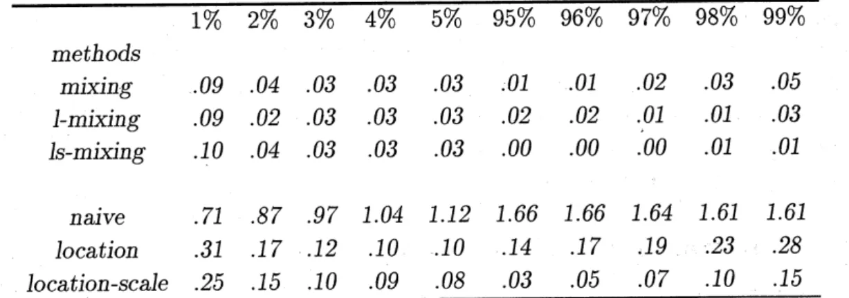
Let$X$ and$Y$comefromthenull$F=N(\mu_{0}, \sigma^{2}),$ $G=N(\mu_{0}, \sigma^{2})$. Let$m=n=5$ .

Then $H_{0}(t)=t_{8}$ The first row of Table 1 shows the relative errors of the mixed

bootstrap in approximating the lower and upper quantiles of $t_{8}$. As a comparision,

the fourth row corresponding to the naive bootstrap test is also displyed.

The idea of mixing isnot entirelynew. Boos, Janssenand Veraverbeke(1989)

dis-cussesthe pooled bootstrap tests for testing homogeneityof scales, which essentially

(3)

the same

mean

is by location transformation. Efron and Tibshirani($1993$, pp.224)

suggests that the bootstrap samples be drawn from $\{x_{1}’’, \cdots, x_{m}\}$ and $\{y_{1}’, \cdots, y_{n}’\}$,

where the $x’\mathrm{s}$ and $y’\mathrm{s}$ are location adjusted. They are defined as $x_{i}’=x_{i}-\overline{x}+\overline{z}$

and $y_{i}’=y_{i}-\overline{y}+\overline{z},$ where $\overline{x}$ and $\overline{y}$ are the respective sample means and

$\overline{z}$ is the

pooled mean. The fivth rowof Thable 1 shows that this does not work well enough.

The location-scale transformation, by redefining the $x’\mathrm{s}$ and $y’\mathrm{s}$ as $x_{i}’=(x_{i}-\overline{x})/S_{x}$

and $y_{i}’=(yi^{-\overline{y})}/S_{x}$, where $S_{x}$ and $S_{y}$ arethe sample standard errors, improves the

location transformation, but only mildly, see the last row of Table 1. The second

and the third row ofTable 1 compare the mixed bootstrap tests when location or

location-scaletransformation is applied before mixing, with simple mixed bootstrap

test(first row). The results are essentially the same, with moderate improvements

by including transformations.

Table 1 Errorsin approximatingthetails ofthe null distribtionbysixbootstrap

tests. The null distribtion of$T$under nomalitywithhomogeneous scales, is$t_{5+5-2}=$

$t_{8}$. The bootstrap tests use data from a “local alternative”, $N(1,1),$

$N(\mathrm{O}, 0.9^{2})$. 1% 2% 3% 4% 5% 95% 96% 97% 98% 99% methods mixing .09 .04 .03 .03 1-mixing .09 .02 .03 .03 $l\mathrm{s}$-mixing .10 .04 .03 .03 .03 .01 .01 .02 .03 .05 .03 .02 .02 .01 .01 .03 .03 .00 .00 .00 .01 .01 naive .71 .87

.97

1.04 1.12 1.66 1.66 1.64 1.61 1.61 location .31 .17 .12 .10 .10 .14 .17

.19

.23. .28

$\underline{loc\mathrm{a}}$

tion-scale.25.15.10.09.08.03.05.07.10.15

Notes: $(l)The$ figu$\mathrm{r}es$ are $rel$ative errors defined by $|(w-\hat{w})/w|,$ $w$ and

$\hat{w}$ stands

for th$e$ true value and approximate value respectively; (2)$mixi\mathrm{n}g,$

$\mathit{1}$-mixing and

ls-mixin$g$stand for th$e$mixed bootstrap, mixed bootstrap afterlocation and

location-scale transformation, respectively; naive, location and location-scale stand for th$e$

$\mathrm{n}$onmixed bootstrap, nonmixed bootstrap with location and location-scale

$t$

rans-formation, respectivelyj (3)$Th\mathrm{e}$ bootstrap values are averages during 100 repeated

$s$ampling, with each bootstrapped 200 times.

Similarfeaturesare observedfromTable 2, where thenull distribution of$T$based

on $F=N(\mu_{0}, \sigma_{1}^{2})$ and $F=N(\mu 0, \sigma_{2}^{2}),$ $\mu 0=1,$ $\sigma_{1}^{2}=1,$ $\sigma_{2}^{2}=4$ are approximated by

(4)

Table2 Errors in approximatingthe tails ofthe null distribtionbysix bootstrap

tests. The null distribtion of $T$ is defined by assuming _{$X\sim N(1,1)$} and $Y\sim$

$N(1,2^{2})$, sample sizes

$m=n=5$

. The bootstrap tests use _{data from a “local}

alternative”, $N(1,1),$$N(2,2^{2})$. 1% 2% 3% 4% me$th_{\mathit{0}}\mathrm{d}_{S}$ mixing .08 .08 .05 .02 1-mixing .09 .08 .04 .03 $ls$-mixing .03 .07 .04 .01 5% 95% 96% 97% 98% 99% .03 .06 .06 .07 .06 .06 .02 .06 .06 .06 .06 .08 .02 .05 .04 .04 .03 .02 naive 1.64 1.38 1.38 1.40 1.40 .79 .74 .67 .62 .46 location .34 .19 .18 .18 .17 .23 .25 .28 .32 .48

$\underline{loc\mathrm{a}}$

tion-scale.11.03.04.05.03.02.01.03.07.13

Notes: $(l)The$ figures are _relative errors _{defined by} $|(w-\hat{w})/w|,$ $w$ and $\hat{w}$ stands

for the $tr\mathrm{u}e$ value and approximate $\mathrm{r}^{\gamma}\mathrm{a}lue$ respecti

$\iota^{\gamma}\mathrm{e}ly,\cdot(\mathit{2})\mathrm{m}ix\mathrm{j}ng,$ $\mathit{1}$

-mixing and

ls-mixingstand for the mixed bootstrap, mixed bootstrap after location and

location-scale transformation, respecti$\mathrm{r}^{r}\mathrm{e}ly,\cdot$ naive, location and location-scale stand for th

$\mathrm{e}$

nonmixed bootstrap, nonmixed bootstrap with location and location-scale

trans-formation, resp$\mathrm{e}cti\gamma \mathrm{e}ly,\cdot(\mathit{3})Th\mathrm{e}$ bootstrap values are averages during 100 repeated

sam.pling,

with $e\mathrm{a}ch$ bootstrapped 200 times; (4)$Then\mathrm{u}\mathit{1}\mathit{1}$ distribution is

approxi-mated by 5,000 Monte Carlo trials.

3 Bootstrap Tests

of

Darwin’s

Zea Data

Table _{3 shows data obtained by Darwin(1876), who investigated whether there}

exists superiority of the crossed plantsover the self-fertilized. The data shown here

concernsonly$\mathrm{z}\mathrm{e}\mathrm{a}$, oneout of the

seven

plantsexperimentedbyDarwin. The problem

is to test the null hypothese $H_{0}$ : _{$\mu_{X}=\mu_{Y}$} against the alternative $H_{1}$ : _{$\mu_{X}>\mu_{Y}$},

where $\mu_{X}$ and $\mu_{Y}$ represent the mean height of the crossed and the self-fertilized

$\mathrm{z}\mathrm{e}\mathrm{a}$, respectively.

While the nonmixed bootstrap with location transformation applied to the zea

datagives one-sided achievedsignificance level$(\mathrm{a}.\mathrm{S}.1.)$ 0.043, the simple mixed

boot-strap has a.s.l. 0.012, providing much stronger evidence against the null hypothesis

that there is no difference between the crossed and self-fertilized $\mathrm{z}\mathrm{e}\mathrm{a}$. In mixing

is done after location transformation, the a.s.l. decreases to 0.006, indicating even

more discrepancy between the two kinds of$\mathrm{z}\mathrm{e}\mathrm{a}$. Location-scale transformation does

not have much effect in the mixing case(with a.s.l. 0.011), but reduces the a.s.l. to

(5)

bootstrap samples in the mixed and nonmixed cases, respectively. For

compari-sion, the two-sided a.s.l.’s of some conventional nonparametric tests, namely the

median, Wilcoxson and permutation test are 0.001, 0.003 and 0.024, respectively,

see Takeuchi and Ohasi(1981) for details.

Table 3 Darwin’s observations on-the grouth rates ofthe crossed and

self-fertilized $\mathrm{z}\mathrm{e}\mathrm{a}$. Numbers are expressed in eighthsof an inch.

$NO\acute{T}ES$: The data can be found in Fisher($\mathit{1}\mathit{9}\mathit{6}\mathit{0}$, pp.30), which are divided into bloks

of sizes (3,3,5,4), corresponding to each pot. For exampl$\mathrm{e},$

$(\mathit{1}\mathit{8}\mathit{8},\mathit{9}\mathit{6},\mathit{1}\mathit{6}\mathit{8})$ and (139,

163, 160) are from pot 1, and (168, 177,184, 96) and (144, 102, 124, 144) are from

pot 4, etc.

4 Stratified

Sampling

In this section,we treatgeneralstratifiedproblems, assuming$F(x)= \sum_{l=1}LF_{l}(w_{l}x)$

and $G(y)=\Sigma_{h=1}^{H}p_{h}G_{h}(y)$. Here each $F_{l}(x)(l=1, \cdots , L)$ and $G_{h}(y)(h=1, \cdot*\cdot , H)$

represent the l- and h-th stratum distribution functions and $w_{l}(l=1, \cdots, L)$ and

$p_{h}$$(h=1, \cdots , H)$ are the corresponding stratum weights, subject to

$\Sigma_{l=1}^{L}w_{l}=$

$\sum_{h=1}^{H}p_{h}=1$. We only consider the location-aligned bootstrap test.

4.1 The model

Suppose data $\{X_{l1}, \cdots,x_{l}ml\}(l=1, \cdots, L)$ and $\{y_{h1}, \cdots, y_{hn_{h}}\}(h=1, \cdots, H)$,

are observed from each stratum $F_{l}$ and $G_{h}$, respectively. Let $\sum m_{l}=m,$ $\sum n_{h}=n$.

The sample means$\overline{x}_{l}=\sum x_{li}/m_{l}$ and$\overline{y}_{h}=\sum y_{hi}/n_{h}$ are unbiased estimatesforeach

stratummean $\mu_{lX}$ and$\mu_{hY}$, which, combined together, formunbiased

$\mathrm{e}\mathrm{s}\mathrm{t}\mathrm{i}\mathrm{m}\mathrm{a}\mathrm{t}\mathrm{e}\mathrm{s}\overline{x}^{s}=$

$\sum w_{l^{\overline{X}}lX}$ and $\overline{y}^{s}=\sum p_{h\overline{y}_{hY}}$ for the total mean $\mu_{X}$ and $\mu_{Y}$ respectively. Hereafter we

only consider proportional allocation, i.e. $ml=wlm\dot{\mathrm{a}}\mathrm{n}\mathrm{d}nh=phn$.

Let $\hat{\sigma}_{lX}^{2}$ be the usual unbiased version of sample variances of each stratum

vari-ance

$\sigma_{lX}^{2}$. Wakimoto(1971) proved that

$st \hat{\sigma}_{X}^{2}=\sum_{l=1}^{L}w_{l}\hat{\sigma}^{2}l..x+\sum^{L}wl(_{\overline{X}_{l}}l=1-\overline{X}^{S})^{2}-\sum_{=l1}w\iota L(1-wl)\hat{\sigma}_{l}^{2}X/m_{l}$

is unbiasedfor the total variance$\sigma_{X}^{2}$. Theunbiased estimator$st\hat{\sigma}_{Y}^{2}$ for$\sigma_{Y}^{2}$ issimilarly

(6)

The stratified version of the usual $t$-statistic becomes

$T_{st}= \frac{\overline{X}^{S}-\overline{Y}s}{\sqrt{st\hat{\sigma}_{x}^{2}/m+st\hat{\sigma}/2Yn}}$, (4)

based on which we are to test $H_{0}$

:

$\mu_{X}=\mu_{Y}$ against the alternative $H_{1}$ : _{$\mu_{X}>\mu_{Y}$}.

To perform a test $\mathrm{b}\mathrm{a}s$ed on _{$T_{st}$}, is to find, or to make a good approximation

of

$Q(F_{N}, G_{N})=Prob(T_{s}t\leq t)$, the nulldistribution function. To emphasize, we have

deliberately changedour notation using $F_{N}$ and $G_{N}$ in place of$F$ and $G$to represent

the two distributions under null hypothesis, i.e. $\mu_{X}=\mu_{Y}$.

Let $\hat{F}_{l}$ be the empirical

distribution function of the l-th stratum of $F$ putting

mass $1/m_{l}$ on each atom $x_{li}(i=1, \cdot \mathrm{v}\cdot, m_{l})$, and $\hat{G}_{h}$

similarly defined. Define $\hat{F}=$

$\Sigma_{l=1}^{L}w_{l}\hat{F}_{l}$ and $\hat{G}=\sum_{h=1}^{H}p_{h}\hat{G}_{h}$. The naive bootstrap draws i.i.d. stratified samples

with replacement from $\hat{F}$ and $\hat{G}$

, exactly in the same way as the original stratified

samples are drawn from $F$ and $G$, which is as useless as in the simple random case.

4.2 Location-aligned bootstrap

test

The location-aligned bootstrap test constitutes the followingsteps.

(1) Let $\overline{z}=(m\overline{x}^{S}+n\overline{y}^{s})/(m+n)$. Define the pseudo-observations for _$l=$

$1,$

$\cdots,$$L$ and $h=1,$$\cdots,$$H$ by :

$x_{li}^{+}$ _{$=x_{li}-\overline{x}l+\overline{Z}/Lw_{l}$} _{$(i=1, \cdots, m_{l})$}, $y_{hi}^{+}$ $=y_{hi^{-}}\overline{y}h+\overline{Z}/Hp_{h}$ $(i=1, \cdots, n_{h})$.

(2) Define pseudo-empirical distribution functions

$\hat{F}_{N}$ $=\Sigma_{l=1}^{L}w_{l}\hat{F}\iota N$,

$\hat{G}_{N}$ $=\Sigma_{h=1}^{H}ph\hat{G}_{hN}$,

where $\hat{F}_{lN}$ is the empirical

distribution function $\mathrm{p}\mathrm{u}\mathrm{t}\mathrm{t}\mathrm{i}\acute{\mathrm{n}}\mathrm{g}$

mass $1/m_{l}$ on each atom $x_{li}^{+}(i=1, \cdots, m_{l})$, and $\hat{G}_{hN}$ is similar.

(3) Define the bootstrap estimate of$Q(F_{N}, G_{N})$ by $Q(\hat{F}_{N},\hat{G}_{N})$, which is

fur-ther approximated by Monte Carlo means

$\frac{1}{B}\#\{T_{st}^{b*}\leq t\}$,

where $T_{st}^{b*}$ is the version of $T_{st}$, based on the b-th stratified samples from $\hat{F}_{N}$ and

$\hat{G}_{N},$ $\#$ stands for the number of the event within

$\{\}$ being true and $B$ is the number

of the whole procedure replicated. Several remarks are pertinent.

Remark _{1 To reflect the null hypothesis, namely two} _{distributions} _{sharing the}

(7)

null hypothesis does pose some restictions on the second order moments, as in the

case of approximating the $t$-distribition discussed in Section 2, proper adjustments

upto that order may to be prefered. Empirical variances may be adjusted in the

stratified case as following

$x_{li}^{o}$ $=[(x_{li^{-}}\overline{x}_{l})/S_{lx}](1/L\sqrt{w_{l}})+1/w_{l}L\sqrt{m}$ $(i=1, \cdots, m\iota)$, $y_{hi}^{o}$ $=[(y_{hi}-\overline{y}_{h})/s_{hy}](1/H\sqrt{p_{h}})+1/p_{h}H\sqrt{n}$ $(i=1, \cdots, n_{h})$.

Thistransformation is exact when $(m+1)/(n+1)=H/L$ , whichis satisfied, for

ex-ample, when $m=n$ and $L=H$. We will not considerlocation-scale transformation

in our Monte Carlo studies.

Remark 2 Confidence intervals based on asymptotically pivotal quantities tend

to be long-shaped. A 95% bootstrap-t confidence interval for the difference

be-tween the crossed and self-fertilized zea in Example 1 is (1.8, 32.3), compared with

the so-called nonparametric ABC interval(Efron and Tibshirani 1993), (5.5, 29.4).

Welch’s solution gives (3.1, 44.5), Fisher’s fiducial interval is (2.7, 39.1), compared

with $(13, 39)$ _which is based on Wilcoxsontest($\mathrm{T}\mathrm{a}\mathrm{k}\mathrm{e}\mathrm{u}\mathrm{c}\mathrm{h}\mathrm{i}$ and Ohasi 1981, $\mathrm{p}\mathrm{p}.51^{-}89$).

One consequence ofthis is that $‘(t$-type” tests may tend to have lower power.

5 Monte Carlo Studies

Assume that the data do come from distributions satifying the null hypothesis

and $t_{0}$ is the observed value of the stratified $t$-statistic. The achieved significance

level,or$p$-value, Prob$(\tau_{St}>t_{0})$ undernullhypothesisdependssolelyon$t_{0}$, which has

theuniform distribution on $(0,1)$ if$t_{0}$ israndomlyobservedfrom thenull hypothesis.

We shall evaluate our bootstrap tests by checking the size, power and testing the

uniformity of the p-values.

Now the hypothesis $H_{0}$

:

_{$\mu_{X}=\mu_{Y}$} is to be tested against the alternative $H_{1}$ :

$\mu_{X}>\mu_{Y}$, based on the location-aligned bootstrap test described in the previous

section. For simplicity, we assume $F$ and $G$ in the following simulations to be

mixtures of two normal populations, and $w_{l}=p_{l}(l=1,2)$. With noloss ofgenerality,

we fix $\mu_{Y}=1$ and varify the following quantities: coefficient of variations, $C_{X}=$

$\sigma_{X}/\mu_{X},$ $C_{Y}=\sigma_{Y}/\mu_{Y}$; ratio of (sub-)variances, $S_{X}=\sigma_{2X}^{2}/\sigma_{1}^{2}\mathrm{x}’ S_{\mathrm{Y}}=\sigma_{2Y}^{2}/\sigma_{1Y}^{2}$; and the effect of stratifications, $\rho_{X}^{2}=\Sigma_{l=1}^{2}(\mu_{1}X -\mu_{2X})^{2}/\sigma_{X}^{2},$ $\rho_{Y}^{2}=\sum_{l=1}^{2}(\mu_{1}Y$

-$\mu_{2Y})^{2}/\sigma_{Y}^{2}$. To fully specify $F$ and $G$we need one more condition, which is designed

so that the test is supposed to have approximate power (0.2, 0.4, 0.6, 0.8). This

constraint is derivedby approximatingthe bootstrap distribution of$T_{st}^{*}$ by thelimit

$N(0,\sigma^{2}(1-\rho Y)^{)N(}2A\sigma^{2}Y\mathrm{o}\mathrm{f}/n]\tau_{s/(}t\mathrm{u}_{2}\mathrm{n}\sigma_{X}\mathrm{d}/\mathrm{e}\mathrm{r}Hm+\sigma_{Y}^{2}0\mathrm{a}\mathrm{n}/n),$$\mathrm{a}\mathrm{n}\mathrm{d}\delta=(\mu X^{-}\mu_{Y}\mathrm{d}\delta,$$\sigma_{A}^{2})\mathrm{u}\mathrm{n}\mathrm{d}\mathrm{e}\mathrm{r}H1,)/\mathrm{W}\mathrm{h}\mathrm{e}_{2}\mathrm{r}\mathrm{e}\sigma\infty\sigma_{x}/m+\sigma_{Y}/2n2=(1.-\rho X)2\sigma_{x}/2m+$

Table 4shows relativegoodbehaviourofthelocatio-aligned bootstrap test,when

(8)

The lower half of this table displaysthe results ofthe same bootstrap test when the

stratified samples are treated as simple random samples, losses ofpower in the later

case are observed.

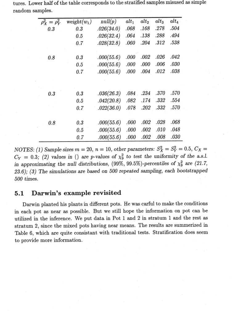
Table 4 10%-1evel location-aligned bootstrap tests applied to normal mixtures.

The sample sizes are $m=n=10$, effects of stratification, $\rho_{X}^{2}=\rho_{Y}^{2}=0.3$. The

bootstrap tests approximately achieve thenorminal level(O.l), and have reasonable

power. Lower half of the table corresponds to the stratified samples misused as

simple random samples.

$\overline{\mathrm{t}Veight(w_{1})}$

case $null(p)$ $alt_{1}$ $alt_{2}$ $alt_{3}$ $alt_{4}$

0.3 $I$ .086(13.1) .164 .384 .524

.758

II .118(13.5) .150 .354 .512 .718 0.5 $I$ .080(6.4) .146 .312 .486 .722 II .094(4.8) .162 .278 .460 .682 0.7 $I$ .090(9.1) .138 .368 .540 .768 II .086(12.0) .186 .322 .520 .714 0.3 $I$ .070(13.0) .134 .322 .458 .710 II .078(8.7) .096 .276 .464 .630 0.5 $I$ .072(14.7) .130 .290 .496 .712 II .054(17.8) .132 .240 .414 .612 0.7 $I$ .060(22.4) .104 .312 .494 .736 II .044(24.8) .096 .202 .370 .598

NOTES: (1) CaseI and II correspondto theparameter layou$tS_{X}=S_{Y}=0.5,$ $C_{X}=$

$C_{Y}=0.3$ and $S_{X}=S_{Y}=1,$ $C_{X}=0.3,$ $C_{Y}=0.8,$ $\mathrm{r}\mathrm{e}sp\mathrm{e}cti_{Ve}ly,\cdot(\mathit{2})$ values in $()$

are $p$-values of $\chi_{9}^{2}$ to test the uniformity of the a.s.l. in approximating th

$\mathrm{e}$ null

distributions, (90%,

95%)-percentiles

of$\chi_{9}^{2}$ being (14.7, 16.9); (3) The simulations

are based on

500

repeated sampling, each bootstrapped 500 times.

Location-aligned bootstrap tests are however quite sensitive to the effects of

stratification $(\rho_{X}^{2}, \rho_{Y}^{2})$, and to the balance of samples, as can be seen from Table 5.

To improve, ideas like mixing may be incorporated, weleave the experiments as our

(9)

Table 5 10%-level location-aligned bootstrap tests applied to two normal

mix-tures. Lower half of the table corresponds to the stratified samples misused assimple

random samples. $\overline{\rho_{X}^{2}=\rho_{Y}^{2}\iota \mathrm{v}e\mathrm{j}ght(w1)null(p)alt_{1}alt2alt_{3}alt4}$ 0.3 0.3 .026(34.0) .068 .168 .278 .504 0.5 .026(32.4) .064 .138 .288 .494 0.7 .028(32.8) .060 .204 .312 .538 0.8 0.3 .000(55.6) .000 .002 .026 .042 0.5 .000(55.6) .000 .000 .006 .030 0.7 .000(55.6) .000 .004 .012 .038 0.3 0.3 .036(26.3) .084 .234 .370 .570 0.5 .042(20.8) .082 .174 .332 .554 0.7 .022(36.0) .078 .202 .332 .570 0.8 0.3 .000(55.6) .000 .002 .028 .068 0.5 .000(55.6)

.000

.002

.010 .048

0.7

.000(55.6) .000

.002 .008 .030

NOTES: (1) Sample sizes $m=20,$ $n=10,$ $oth$erparameters: $S_{X}^{2}=s_{Y}^{2}=0.\mathit{5},$ $C_{X}=$

$C_{Y}=0.3;(\mathit{2})$ values in $()$ are $p$-values of $\chi_{9}^{2}$ to test the uniformity of the a.s.l.

in approximating the $m\mathrm{z}\mathit{1}\mathit{1}$ distributions, (99%, 99.5%)-percentiles of$\chi_{9}^{2}$ are (21.7,

23.6); (3) The simulations are based on

500

repeated sampling, each bootstrapped

500 times.

5.1 Darwin’s

example

revisited

Darwin planted his plantsin different pots. Hewas carful to make the conditions

in each pot as near as possible. But we still hope the information on pot can be

utilized in the inference. We put data in Pot 1 and 2 in stratum 1 and the rest as

stratum 2, since the mixed pots having near means. The results are summerized in

Table 6, which are quite consistant with traditional tests. Stratification does seem

(10)

Table 6. Bootstrap tests of the difference on growth rates between the

crossed-andself-fertilized$\mathrm{z}\mathrm{e}\mathrm{a}$. Thefiguresaretwo-sided achieved significance levels, obtained

from 200bootstrap samples. Other _{classical parametric and nonparametric tests}_are

alsoshown(Takeuchiand Ohasi, 1981). Among thesetests, themedian test has least

a.s.l., the corresponding 95% confidence interval is $(1\mathit{9}, 45)$, which is “significantly”

short. See Remark 2 od Section 4.2.

Method Type of Transformation asl

no transformation .505

stratiBed sampling location .000(.005)

location-scale .015(.005) simple no transformation .545 randon location .025(.010) $\frac{s\mathrm{a}mplingl_{\mathit{0}}C\mathrm{a}tion-_{8Ca}le.\mathit{0}\mathit{0}\mathit{5}(.\mathit{0}\mathit{0}5)}{N(\mu_{x},\sigma^{2}),N(\mu_{y},\sigma^{2}).\mathit{0}\mathit{2}}$ one-sample $t(d.f.=n- \mathit{1})$ .05 Wilcoxson _.003 permutation _.024 median .0014

NOTES: $(l)s_{tr}at\mathrm{a}$areformedbymixing Pot 1 and2, andPot2and$\mathit{3};(\mathit{2})N(\mu_{x}, \sigma^{2}),$ $N(\mu_{y}, \sigma^{2})$

stands for the method based the normal assumptions with homogeneous variancesj

one-sample$t(d.f.=n- l)$ forFisher’s one-sample$t$-testby properlypairing th$\mathrm{e}d\mathrm{a}t\mathrm{a}(See$

Fisher, 1960); Wilcoxson for Wilcoxson test; $p$ermutation for$p$ermutation test; and

median for median test; (3)$Figu\mathrm{r}es$ in bracketsare obtained from mixin

$g$ the

trans-formed data in simple random sampling, but only mixing the transtrans-formed data

within $e\mathrm{a}ch$population in stratifi_$ed$ situations.

6 Discussions

Bootstrap tests are statistical procedures _{for seeking information about models}

in _{one class(the null class), conditional on information about a different class(}$\mathrm{t}\mathrm{h}\mathrm{e}$

al-ternative class). In a strict sense, we neverhave direct information of the first class,

but always observe instead information of the latter class. “Validity” of the

trans-formations ofthe $ma\Gamma \mathrm{l}\mathrm{n}\mathrm{f}\mathrm{o}\mathrm{r}\mathrm{m}\mathrm{a}\mathrm{t}\mathrm{i}\mathrm{o}\mathrm{n}$ into the information we want,

obviously depends

(11)

参考文献

[1] Boos, D., Janssen, P. andVeraverbeke, $\mathrm{N}.(1989)$. Resamplingfrom centereddata

in the two-sample problerm, Journal

of

Statistical Planning and Inference, 21,

327-345.

[2] Darwin, $\mathrm{C}.(1876)$, The

effects of

cross- and

self-fertilisation

in the vegetable

kingdom, London: John Murray.

[3] Efron, B. and Tibshirani, $\mathrm{R}.(1\mathit{9}\mathit{9}3),An$Introduction to the Bootstrap: Chapman

and Hall.

[4] Fisher, $\mathrm{R}.\mathrm{A}.(1\mathit{9}60)$, The Design

of

Experiments(

$7\mathrm{t}\mathrm{h}$ ed.), Edinburgh: Oliver and

Boyd.

[5] Takeuchi, K. and Ohasi,$\mathrm{Y}.(1981)$, Toketekisuisoku-2$hy_{\mathit{0}}honmondai$($\mathrm{i}\mathrm{n}$Japanese),

Tokyo: Nihonhyoronsya.

[6] Wakimoto, $\mathrm{K}.(1971)$, Stratified random sampling (I), Estimation ofthe